Machine Learning-Based Real-Time Prediction of Formation Lithology and Tops Using Drilling Parameters with a Web App Integration

Abstract

The accurate prediction of underground formation lithology class and tops is a critical challenge in the oil industry. This paper presents a machine-learning (ML) approach to predict lithology from drilling data, offering real-time litho-facies identification. The ML model, applied via the web app “GeoVision”, achieves remarkable performance during its training phase with a mean accuracy of 95% and a precision of 98%. The model successfully predicts claystone, marl, and sandstone classes with high precision scores. Testing on new data yields an overall accuracy of 95%, providing valuable insights and setting a benchmark for future efforts. To address the limitations of current methodologies, such as time lags and lack of real-time data, we utilize drilling data as a unique endeavor to predict lithology. Our approach integrates nine drilling parameters, going beyond the narrow focus on the rate of penetration (ROP) often seen in previous research. The model was trained and evaluated using the open Volve field dataset, and careful data preprocessing was performed to reduce features, balance the sample distribution, and ensure an unbiased dataset. The innovative methodology demonstrates exceptional performance and offers substantial advantages for real-time geosteering. The accessibility of our models is enhanced through the user-friendly web app “GeoVision”, enabling effective utilization by drilling engineers and marking a significant advancement in the field.

1. Introduction

Since the early days of the oil industry, human ingenuity has been at work to overcome various challenges. Among these challenges, real-time and precise determination of the tops of the formation and its lithology whereas drilling is of utmost importance to guarantee efficient and safe drilling operations [1]. Accurate information about the formation tops is essential when designing a casing program, as it is necessary to select the right depths for placing the casing to ensure efficient zonal separation, and to correctly design the correct mud weight in order to keep the wellbore conditions in check [2,3,4].

Drilling engineers in oil fields use four distinct methods to identify different reservoir zones or formation tops: rate of penetration (ROP) charts, gamma-ray (GR) logs, formation cuttings, and mud logging [5,6,7]. These techniques are helpful for drillers to delineate the formation tops, but each one has drawbacks such as high costs, lower accuracy, and substantial labor. Moreover, the majority of these measurements encounter temporal or depth-related delays, which restrict the ability to instantly estimate the formation tops. These limitations pose challenges to the feasibility and efficacy of current techniques employed for formation top determination.

Although lithology significantly impacts the ROP, other drilling parameters also exert considerable influence on ROP fluctuations [8]. Consequently, relying solely on ROP for estimating lithology changes or formation tops is inadequate, particularly when other drilling parameters experience significant variability. Furthermore, as the wellbore depth increases, there is a noticeable time lag in obtaining geophysical logs or drilled cuttings, which delays the prediction of the currently drilled formation [6]. Employing techniques such as GR, measurement, or logging while drilling, or mud logging in each section is also economically impractical and does not offer prompt and essential information.

On the other hand, to address these challenges, researchers from the realm of the oil and gas industry have harnessed the power of ML to transform key aspects of this industry. In drilling optimization, Berrehal et al. (2022) [9] proposed an ML-based approach for a real-time mechanical earth model, enhancing wellbore stability in the Volve field. Similarly, Al-Sudani et al. (2017) [10] introduced a control engineering system for real-time monitoring of drilling mechanical energy and bit wear, optimizing drilling performance. Meanwhile, for fracturing, Erofeev et al. (2021) [11] predicted post-hydraulic fracturing oil and liquid production with 80% accuracy, enabling real-time HF candidate selection. In the domain of oil recovery, Ouadi et al. (2023) [12] introduced high-accuracy models for predicting gas well productivity using Fishbone drilling, demonstrating its potential to enhance hydrocarbon recovery and reduce environmental impact. Although Ahmed et al. (2017) [13] showcased the potential of AI techniques in estimating oil recovery factors in early-time reservoirs, surpassing existing correlations. Additionally, Hamadi et al. (2023) [14] presented a robust machine-learning framework to predict key parameters in CO₂ -enhanced oil recovery, delivering superior accuracy and insights for efficient CO₂-EOR design. Furthermore, Mouedden et al. (2022) [15] proposed FIScreT, a decision-making tool based on fuzzy logic for automating candidate well selection in stimulation processes.

In this paper, we propose an ML-based approach for real-time lithology prediction from drilling data. The results show a remarkable accuracy of 95% in identifying the claystone, marl, and sandstone. Leveraging multiple drilling parameters and the open Volve dataset, our methodology enables real-time lithofacies classification without time lags, significantly advancing geosteering capabilities.

2. Literature Review

Lithology prediction using machine learning has rapidly evolved from early foundational models to an array of sophisticated techniques, integrating real-time data and achieving high accuracy. The initial explorations into the field of lithology prediction were laid by Rogers et al. (1992) [16], Benaouda et al. (1999) [17], and Wang and Zhang (2008) [18]. Utilizing well-log data, these pioneers developed predictive models; however, they faced challenges in predicting thin formations and dealing with missing density logs. As the field progressed, Qi and Carr (2006) [19] and Al-Anazi and Gates (2010) [20] contributed to the development of machine-learning models for lithofacies and permeability prediction, using refined artificial neural network (ANN) and support vector machine (SVM) techniques. Moazzeni and Haffar (2015) [21] highlighted the impact of external factors on drilling parameters, revealing the need for further refinement of these machine-learning techniques. Addressing this need, Raeesi et al. (2012) [22], Wang and Carr (2012) [23], and Al-Mudhafar (2017) [24] introduced the use of Artificial Neural Networks (ANNs) and comprehensive integrated workflows, which significantly improved lithofacies classification.

The challenge of real-time lithology prediction during drilling operations was addressed by Mohamed et al. (2019) [25] and Nanjo and Tanaka (2019, 2020) [26], utilizing machine-learning models and image analysis methods. Elkatatny et al. (2019) [27] took a significant step towards real-time prediction, using ANN models to determine formation tops based on drilling parameters. Gupta et al. (2020) [28] designed a real-time machine-learning workflow for lithology prediction during drilling, marking a milestone in the field.

In their research, Zhang and Baines (2021) [29] explored machine-learning models such as ANN, SVM, and CNN, which yielded promising results, especially the 2D CNN combined with PCA feature extraction. Similarly, Wei Zhoucheng et al. (2019) [30] proposed a multi-well lithology identification method that involved feature engineering, machine-learning model training, and optimal model selection. Additionally, Aniyom et al. (2022) [31] demonstrated the potential of ensemble methods to improve lithology prediction performance through the development of a voting classifier machine-learning model.

Several studies have integrated additional features or methods into their models to improve classification performance. Xi Chen et al. (2020) [32] combined the Reducing Error Correcting Output Code algorithm with the Kernel Fisher Discriminant Analysis, outperforming conventional methods. Jiang et al. (2021) [33] introduced a stratigraphic unit as an additional feature, significantly improving lithology classification. Zerui Li et al. (2020) [34] proposed a semi-supervised lithology identification workflow using a Laplacian support vector machine, enhancing classification performance by utilizing feature and depth similarities.

Mou et al. (2016) [35] employed support vector machine models to estimate volcanic lithology in the Liaohe Basin, China, achieving high accuracy. In another study, Moazzeni et al. (2015) [21] accurately predicted formation and lithology in the South Pars gas field, Iran, using artificial neural networks. Similarly, Wang De-ping et al. (2007) [36] attained a 96% correctness rate in predicting lithology in the Bayantala oil field by utilizing an SVM model. These studies focused on specific geological contexts and demonstrated impressive accuracy levels.

Flexible and adaptive models have been explored for lithology prediction. Jia et al. (2012) [37] demonstrated the efficacy of an adaptive neuro-fuzzy inference system for lithology identification from well-log data. Cheng et al. (2010) [38] combined a particle swarm optimization (PSO) algorithm with the least squares support vector machines (LSSVM) for higher precision lithology identification.

Sebtosheikh and Salehi (2015) [39] employed support vector machines (SVMs) with various kernel functions for accurate lithology prediction in a multilayered carbonate reservoir in Iran. Building on this, Avanzini et al. (2016) [40] presented a workflow using cluster analysis to identify productive sweet spots in unconventional reservoirs, focusing on the Barnett Shale Formation. In a different approach, Gu et al. (2019) [41] achieved high (>75%) lithology prediction accuracies by integrating CRBMs and PSO into PNNs. Additionally, Imamverdiyev and Sukhostat (2019) [42] introduced a deep learning 1D CNN model that outperformed other methods in geological facies classification.

Moazzeni et al. (2019) [43] made significant advancements through their research about real-time prediction models by developing an ANN model optimized with a genetic algorithm and Taguchi experimental design for lithology and formation prediction. In a related study, Zhang and Baines (2021) [29] demonstrated the potential of real-time models with their 2D CNN model, achieving over 90% accuracy in identifying four lithology classes. These notable developments have contributed to the progress of real-time prediction techniques.

Finally, recent studies have demonstrated the feasibility of rapid, automated lithology prediction. Popescu et al. (2020) [44] created a supervised machine-learning pipeline that enabled rapid, scalable, and confident lithology prediction. Ao et al. (2019) [45] combined mean–shift feature extraction and random forest classification to improve prediction accuracy. Zhang et al. (2017) [46] used a convolutional neural network for accurate lithology identification from borehole images with a success rate of about 95%.

3. Exploratory Data Analysis

Effective supervised machine learning depends on high-quality data. Meticulous data collection is vital, aiming for near-error-free and pertinent information. Rigorous statistical analysis precedes model development to assess data distribution, remove outliers, and validate parameter relationships. This data-driven approach establishes a strong foundation for accurate and reliable predictive models.

3.1. Data Collection and Description

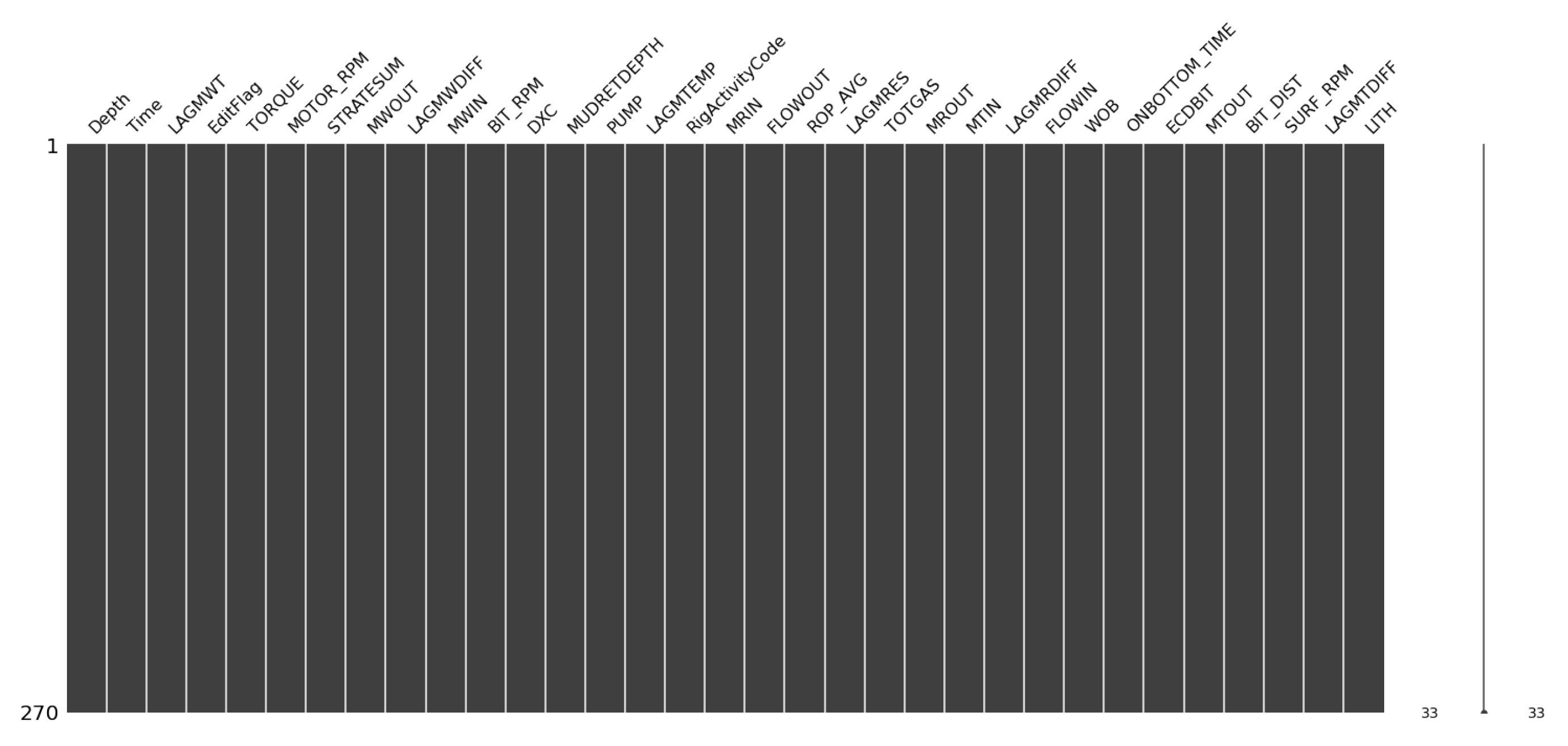
Our analysis revolves around data from two wells originating from Equinor’s open database, more precisely the Volve field in the North Sea. Each well’s dataset comprises 33 columns; 2 columns (Depth and Time) are called the identifiers as we obtain the measurements at each depth in real time, 30 columns are the measured magnitudes obtained from the drilling data with more than 440 observations. Guided by our objective of real-time lithology prediction, we prioritize instantaneous drilling parameters to capture the subsurface formation’s immediate response. Consequently, features like LAGMRES, LAGMRDIFF, and others, which represent lagged or derived measures, were excluded to prevent redundancy and potential multicollinearity. Operational indicators such as EditFlag and RigActivityCode were also omitted due to their lack of direct relevance to formation characteristics. Aggregate measures, like MOTOR_RPM and MTOUT, were discarded to ensure the model’s sensitivity to real-time changes. This targeted selection facilitates efficient and precise modeling, in line with our core objective of immediate formation insight. The last column, abbreviated as LITH, is the lithology label sourced from mud logging data, and as demonstrated in Figure 1, each column consists of 270 rows without any missing values.

Within the dataset, the 30 columns represent.

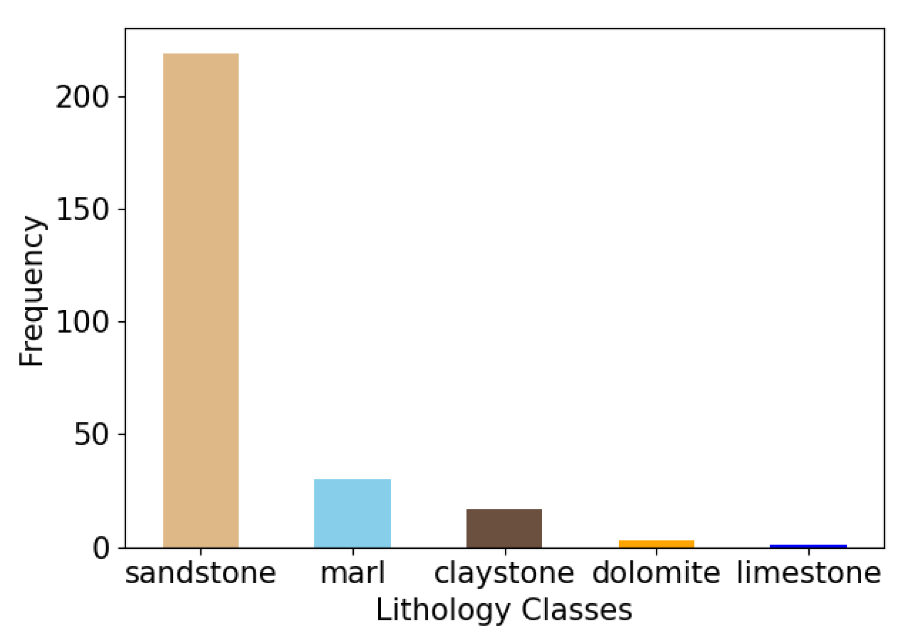
During the investigation of the LITH column, we encountered a diverse array of lithologies, categorized into five distinct classes: sandstone, marl, claystone (shale), dolomite, and limestone (see Figure 2). Given the limited observations for limestone and dolomite, our analysis primarily focused on sandstone, marl, and claystone for classification purposes.

3.2. Oversampling of the Imbalanced Class

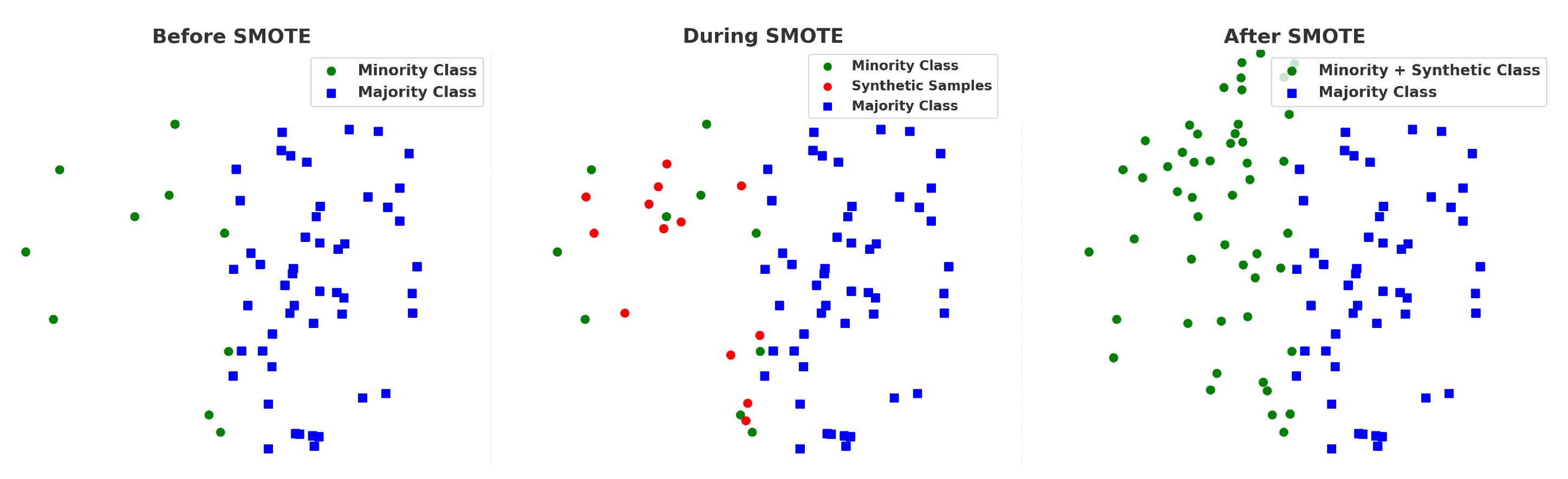
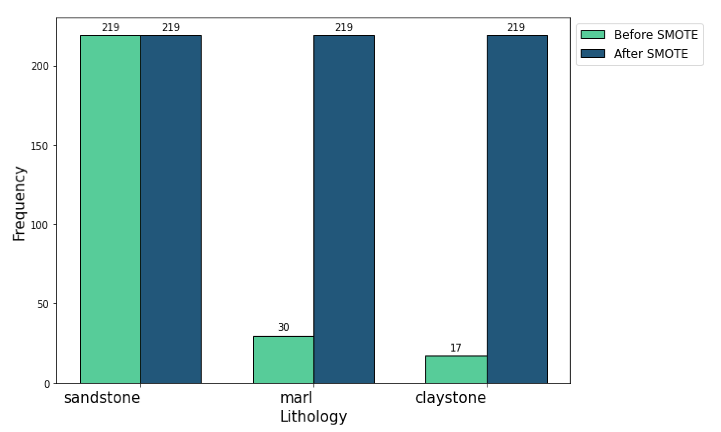
To address the class imbalance in the dataset, we applied the SMOTE technique, which creates synthetic samples for the under-represented classes. Moreover, Insights about this technique from R. Blagus et al. (2013) [47] further guided our approach, as illustrated in Figure 3. Originally, we had 219, 30, and 17 samples for sandstone, claystone, and marl, respectively. After using SMOTE technique, each class was balanced, resulting in 219 samples for each class, as depicted in Figure 4.

The balanced dataset will be later partitioned for modeling after feature selection, with feature variables (X) and the target variable (Y) split in a 70:30 ratio. Consequently, our testing set encompassed 195 samples, with 65 from each class, whereas the training set held the residual 70%. Further details on this process and its outcomes are elaborated in the random forest classifier implementation section.

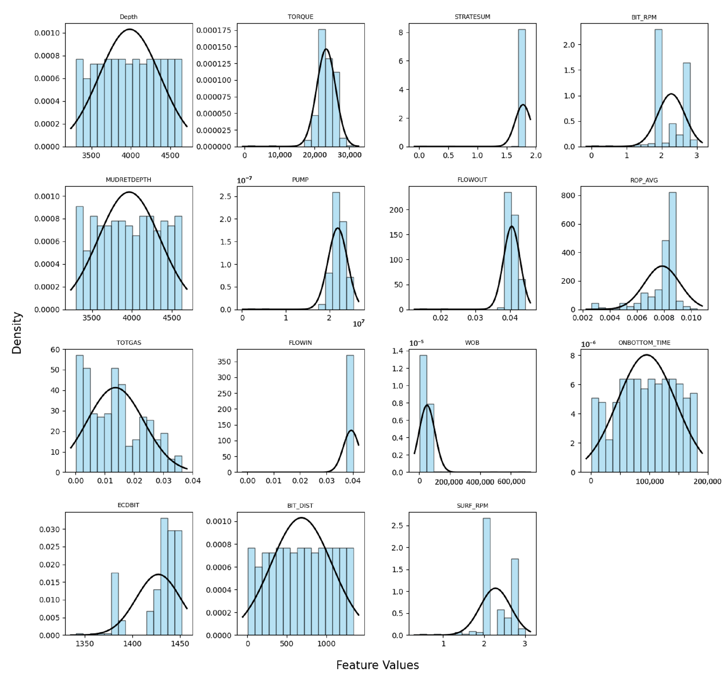
Figure 5 showcases raw data distribution histograms, highlighting the initial step in our approach to predicting underground lithology through drilling data, complemented by a normal distribution curve illustrating a bell-shaped pattern commonly seen in various natural phenomena and statistical processes [49]. These histograms provide a direct visual insight into the distribution patterns. The horizontal coordinates (X-axis) illustrate the feature value range. An example is the “Depth” feature, where the x-axis delineates depths from the dataset’s minimum to maximum values. The vertical coordinates (Y-axis) depict data point frequency within a range. In histograms, the y-axis quantifies the occurrences of specific value ranges in the dataset. This comprehensive visualization of data patterns serves as the foundation for our machine-learning model’s training. By understanding the nuances and variations in parameters like rate of penetration (ROP) and others, we can better tailor our prediction algorithms. Moreover, these distributions shed light on the potential outliers or anomalies that might skew the model’s performance. The raw data distribution graphs, therefore, serve as an initial checkpoint, ensuring that the data we feed into our webb app are not only representative of real-world drilling scenarios but are also devoid of biases that could undermine the model’s predictive capabilities.

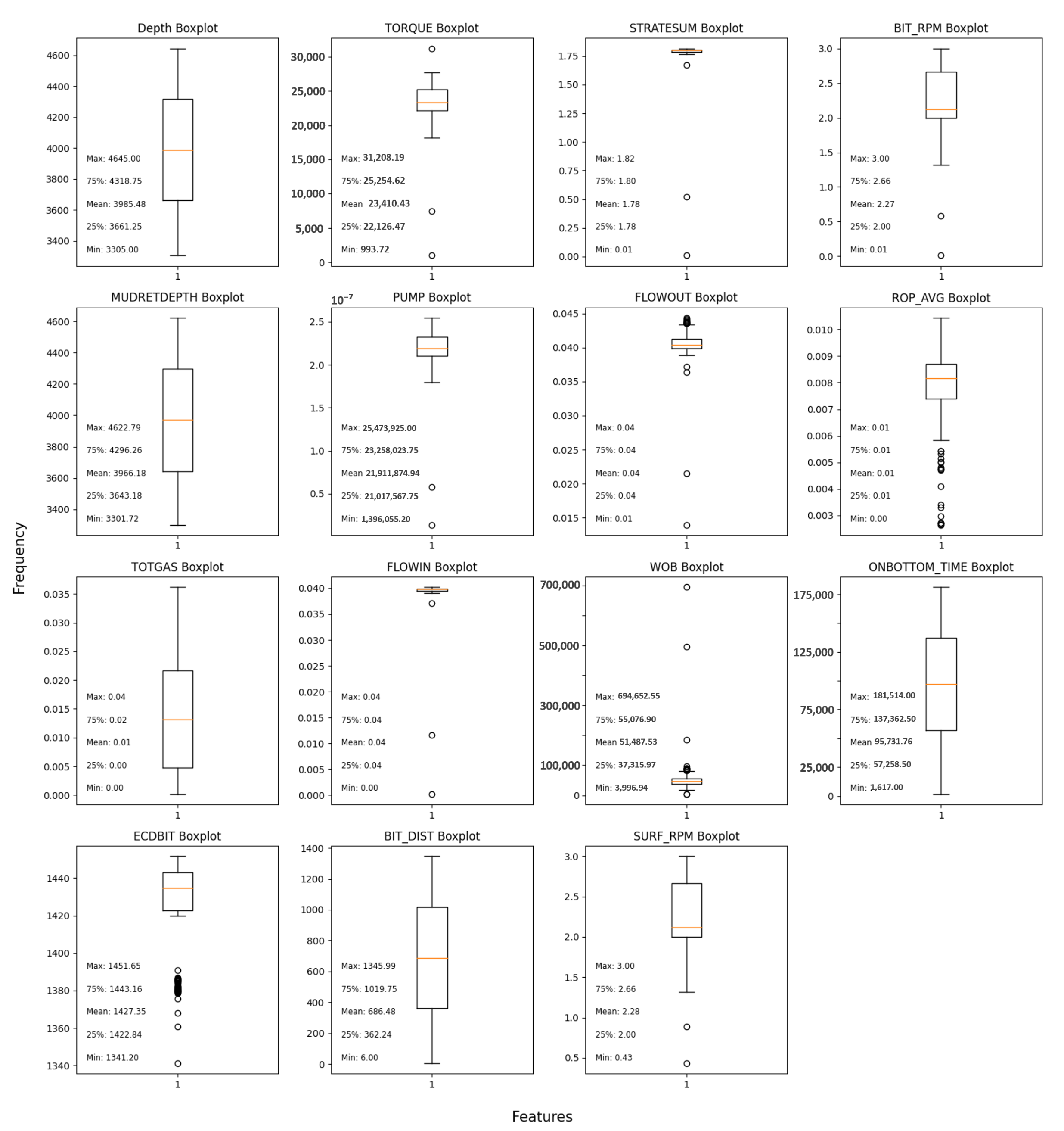
Figure 6 presents box plots before automated outlier removal, showing central tendency and dispersion. Boxes represent the interquartile range (middle 50% of data), with lines indicating medians. Whiskers extend to the minimum and maximum data points (excluding outliers), and relevant statistics are displayed at the top left of each plot.

To ensure the integrity and accuracy of our analysis, it is essential to identify and handle outliers, which are extreme data points that deviate significantly from the majority of the data. Outliers can arise due to various factors such as measurement errors, data entry mistakes, or rare occurrences. If left untreated, outliers can distort statistical analyses, leading to misleading conclusions and unreliable predictions.

To address this issue, we employed the Interquartile Range (IQR) method for outlier detection and removal. For each column, we calculated the first quartile (Q1) and third quartile (Q3) values. The Interquartile Range (IQR) was then determined as the difference between Q3 and Q1. Any data point that fell below (Q1 − 1.5 × IQR) or above (Q3 + 1.5 × IQR) was considered an outlier and subsequently removed from the dataset [50].

By applying the IQR method, we effectively identified and eliminated outliers while preserving the majority of the data that represent the underlying distribution. This approach ensures the robustness and reliability of our analysis, allowing us to draw meaningful insights from the data.

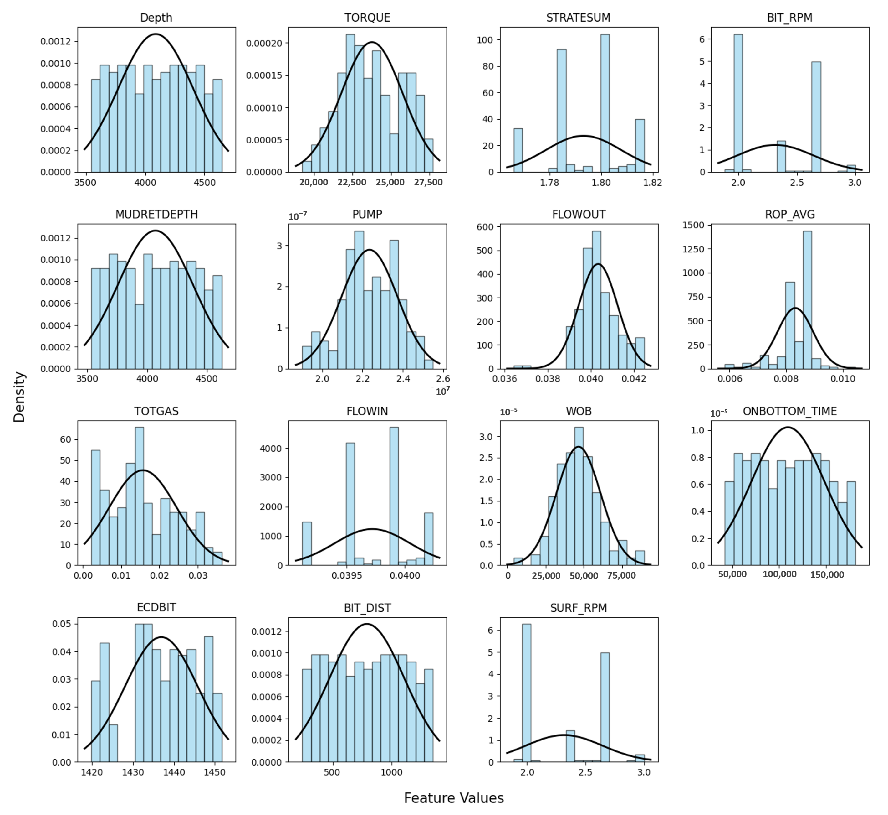
After outlier removal, the distribution may exhibit a more refined and meaningful pattern, which can be observed in the subsequent histograms (Figure 7).

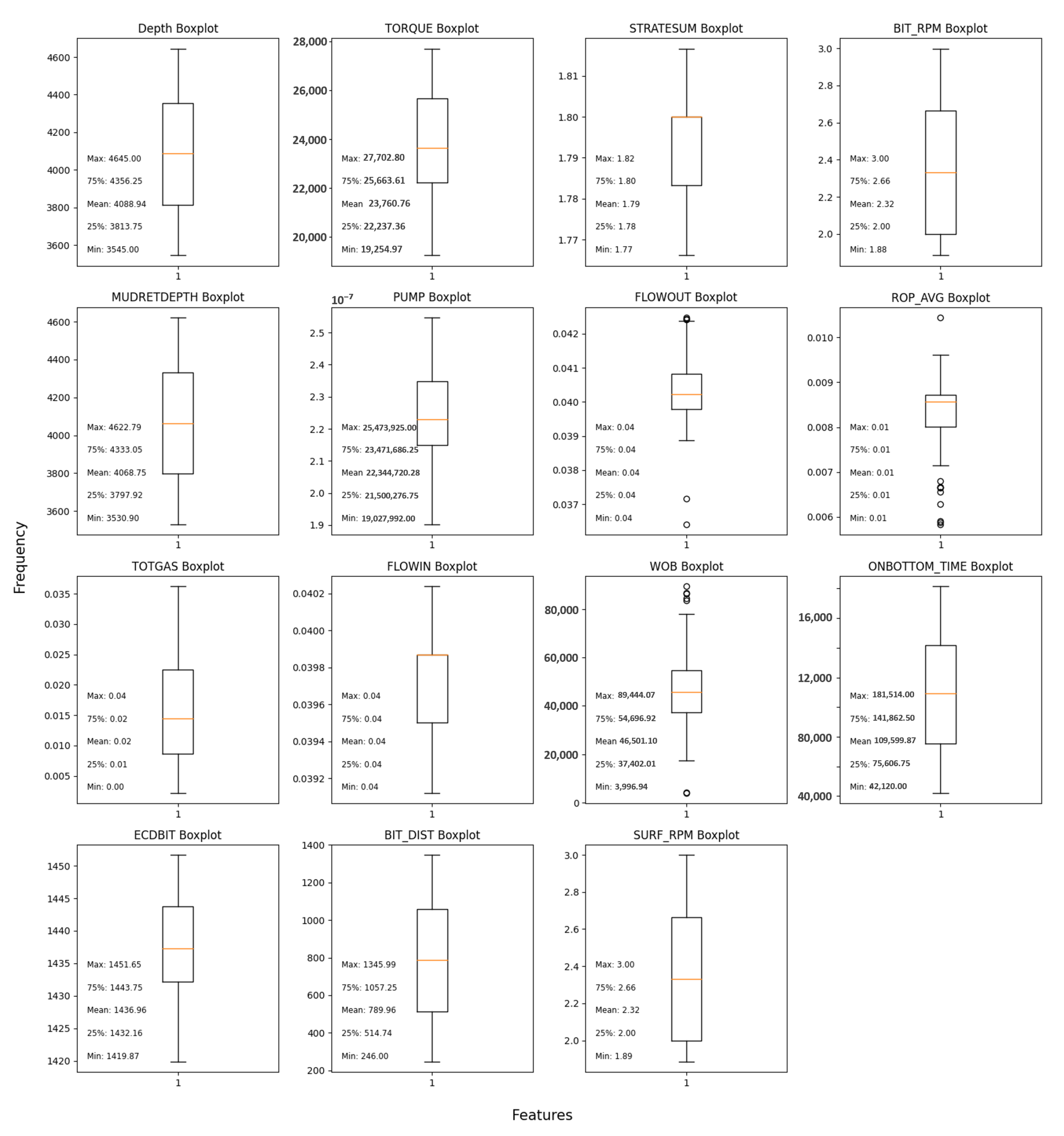
After deploying the Interquartile Range (IQR) method to treat outliers, the boxplots in Figure 8 vividly underscore the dataset’s transformation. Specifically, attributes such as ECDBIT and ROP_AVG now exhibit a tighter and more precise data distribution, clearly indicating the effective removal of extreme values. For instance, the constricted range of ECDBIT suggests a consistent enhancement in drilling efficiency across the dataset. Similarly, the ROP_AVG attribute’s spread has been significantly tightened, reflecting a more uniform average rate of penetration. Moreover, this meticulous data refinement process also rectified anomalies like the physically implausible negative values in the WOB feature. Such diligent data preprocessing not only illuminates central tendency and dispersion more clearly but also sets a robust and reliable foundation for the subsequent predictive modeling stages of our analysis.

For comprehensive details about the features and their corresponding representations, please consult

Table A1. Description and units of drilling parameters.

Attribute	Representation	Unit
Depth	Depth at which drilling is taking place	m
TORQUE	Rotational force applied during drilling	N.m
STRATESUM	Total pump strokes rate	spm
BIT_RPM	Rotation per minute at drill bit	c/s
MUDRETDEPTH	Mud return depth	m
PUMP	Pump pressure	Pa
FLOWOUT	Outgoing mud flow	m3/s
ROP_AVG	Average rate of penetration	m/s
TOTGAS	Total gas content	ppm
FLOWIN	Incoming mud flow	m3/s
WOB	Weight applied to the drill bit	N
ONBOTTOM_TIME	Time since drill bit touched the bottom	s
ECDBIT	Effective circulation density on bit	kg/m3
BIT_DIST	Distance traveled by the drill bit	m
SURF_RPM	Surface rotation per minute	c/s

in Appendix B.

3.3. Feature Selection

During the analysis of drilling data, a substantial number of abbreviated measurements were obtained. To streamline the dataset for further analysis and facilitate faster model training, we conducted feature selection by eliminating erroneous and redundant features, ensuring the integrity of our predictive model.

3.3.1. Erroneous Features

Erroneous features refer to those in the dataset that offer limited or redundant information when classifying the target variable. These features may consist of constant or uniform values, reducing their usefulness in predictive modeling. It is crucial to identify and address such features to optimize the dataset and enhance the efficiency of the predictive model. Descriptive statistics play a pivotal role in detecting erroneous features. Through a thorough examination of the summarized data (see

Table 1. Erroneous features in drilling data.

	Rig Activity Code	DXC	MWIN	LAGMTDIFF
count	266.0	266.00	266.00	266.00
mean	111.0	0.99	1319.80	−286.16
std	0.0	0.00	2.59	69.65
min	111.0	0.99	1280.00	−303.15
25%	111.0	0.99	1320.00	−303.15
50%	111.0	0.99	1320.00	−303.15
75%	111.0	0.99	1320.00	−303.15
max	111.0	0.99	1320.01	0.00

), we can identify features that may necessitate removal or further investigation, ensuring the integrity and accuracy of our analysis.

Several features in the drilling data exhibit constant values, as evident from their identical mean, minimum, maximum, and percentiles. RigActivityCode and DXC fall into this category, rendering them erroneous and unsuitable for meaningful analysis. RigActivityCode appears to be a mere annotation without any informative value, whereas DXC lacks variability, diminishing its relevance in our predictive model. Similarly, MWIN and LAGMTDIFF reveal uniform percentiles along with the maximum and minimum, further confirming their erroneous nature.

Moreover, another approach to identifying erroneous features involves assessing the percentage of data containing zeros. In

Table 2. Percentage of data containing zeros.

Features	Zero Percentages
STRATESUM	0%
MWOUT	0%
LAGMWDIFF	81%
MWIN	0%
BIT_RPM	0%
DXC	0%
MUDRETDEPTH	0%
PUMP	0%
LAGMTEMP	5%
RigActivityCode	0%

, we have calculated the percentages for each feature. Notably, LAGMWDIFF contains a substantial 81% of zero values, solidifying the rationale for eliminating this feature from our dataset.

3.3.2. Redundant Features

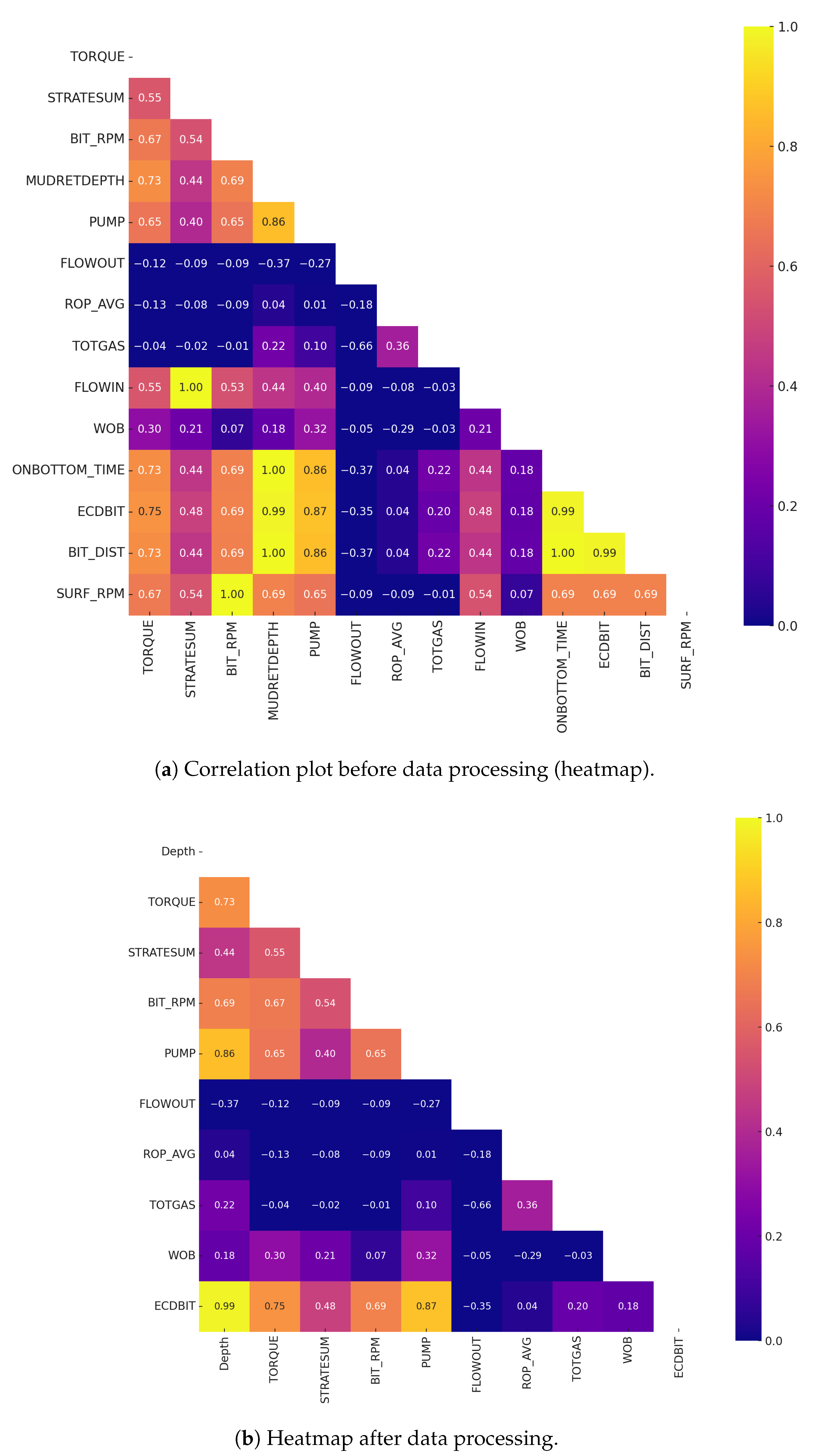
Redundant features have high correlations among them. To quantitatively assess these correlations, a heatmap is plotted using the Spearman correlation method (see Figure 9a), which is a non-parametric measure, is employed to assess monotonic relationships between variables. Its advantage lies in its ability to capture correlations in non-linear datasets, making it suitable for comprehensive analyses in cases where linear relationships might not hold [51].

Upon identifying highly correlated features using Figure 9a, a careful selection process is undertaken to remove redundant variables, supported by domain knowledge. For instance, SURF_RPM (rotation per minute on the surface) is correlated with BIT_RPM (rotation per minute at drill bit) due to the inherent relationship between the rotation measured at the surface and the bit. Consequently, SURF_RPM is excluded from the dataset. Similarly, MUDRETDEPTH, BIT_DIST, and ONBOTTOM_TIME, exhibiting correlations, are removed.

Regarding FLOWIN (incoming mud flow), its association with STRATESUM (total stroke rate) is attributed to the pump measurement received when mud flows in. Thus, FLOWIN is selected for removal. In contrast, FLOWOUT (outgoing mud flow) is found to have no significant correlation with STRATESUM, as the outflow is not determined by the inflow. Consequently, both FLOWOUT and STRATESUM are retained in the dataset for further analysis. To explore the remaining features, refer to Figure 9b for the heatmap after removing redundant features.

3.3.3. Selected Characteristics

After a careful review, we successfully streamlined the initial set of 33 features to a refined selection of 9 key characteristics. The chosen features are as follows:

• TORQUE: Average surface torque (N.m);
• STRATESUM: Total pump strokes rate (spm);
• BIT_RPM: Rotation per minute at drill bit (c/s);
• PUMP: Pump pressure (Pa);
• FLOWOUT: Outgoing mud flow (m³/s);
• ROP_AVG: Average rate of penetration (m/s);
• TOTGAS: Total gas content (ppm);
• WOB: Weight on bit (N);
• ECDBIT: Effective circulation density on bit (kg/m³).

The log-style plot provides valuable insights into the behavior of selected characteristics in relation to changes in lithology types at different depths. Notably, as we drill through the marl formation (represented by the light blue color), we observe an increase in BIT_RPM and WOB. This can be attributed to the nature of marl, which tends to be more compact and challenging to penetrate. As a result, higher rotational speeds and increased weight on the bit are necessary to maintain drilling efficiency and progress through this lithology.

Conversely, during drilling through sandstone (depicted in Beige), we notice an increase in ROP (rate of penetration) and TOTGAS. Sandstone formations often exhibit more porous and permeable characteristics, allowing for smoother drilling operations and higher penetration rates. Additionally, the increase in TOTGAS could indicate the presence of gas-bearing zones within the sandstone, potentially impacting drilling performance (see Figure 10).

Our exploratory data analysis employs the pair plot that visualizes pairwise relationships between different variables in the dataset, segmented by the type of lithology. Each plot shows a different pairing of variables, with histograms along the diagonal representing the distribution of a single variable for each lithology (see Figure 11). It is evident that each lithology type exhibits distinct patterns and relationships between variables, reflecting the unique physical properties of each rock type. However, due to the high dimensionality of the data, further specific analysis is needed to tease out more detailed interpretations of the relationships between variables.

In the next phase of our exploration, we zoom into this expansive landscape and focus on two salient examples, shedding light on the correlations between total gas content and two pivotal drilling parameters, as showcased in Figure 12 and Figure 13.

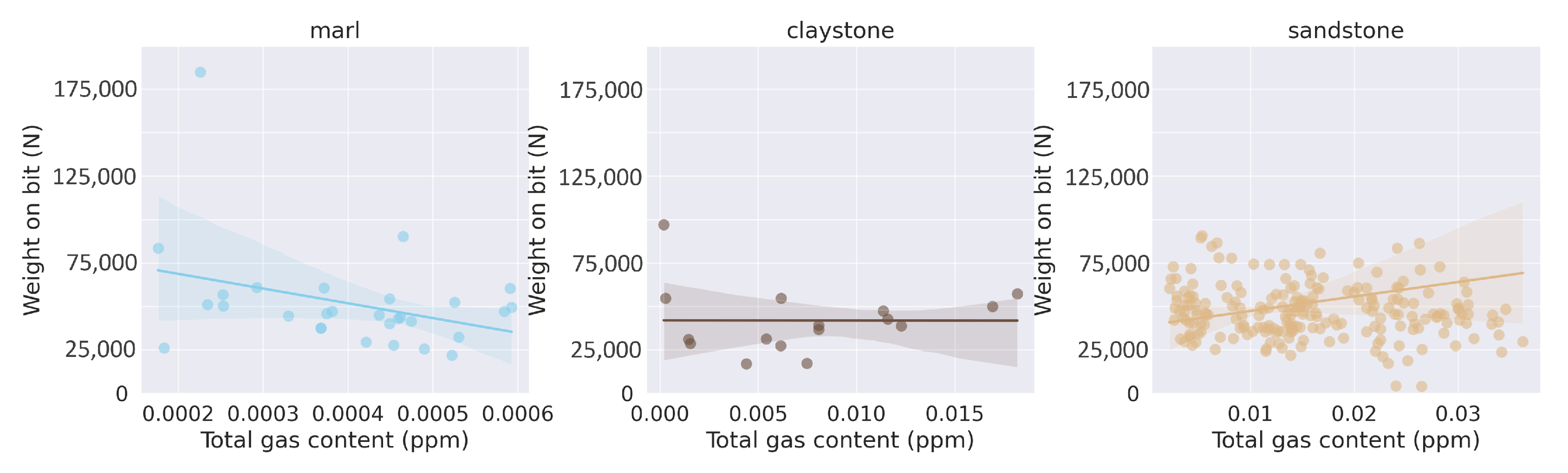
The scatter plots (see Figure 12) demonstrate varying degrees of positive correlation between the total gas content (TOTGAS) and the weight on bit (WOB) across different lithologies. Marl shows a slight positive correlation, claystone exhibits a stronger positive correlation as indicated by the steeper upward-sloping trend line where the points are more closely clustered around the trend line, and sandstone reveals a weak positive correlation due to the wide spread of points. This suggests that the physical characteristics of the lithology, such as porosity, permeability, and gas capacity, could influence the relationship between gas content and weight on the bit. For instance, claystone, which is typically less permeable, might require a higher weight on the bit to achieve efficient drilling, especially in gas-rich sections. Conversely, sandstone, known for its higher porosity and permeability, might allow more efficient gas flow, leading to a less pronounced increase in weight on the bit with higher gas content. However, these are preliminary observations and would require further, more detailed analysis to ascertain the exact nature and significance of the relationships observed.

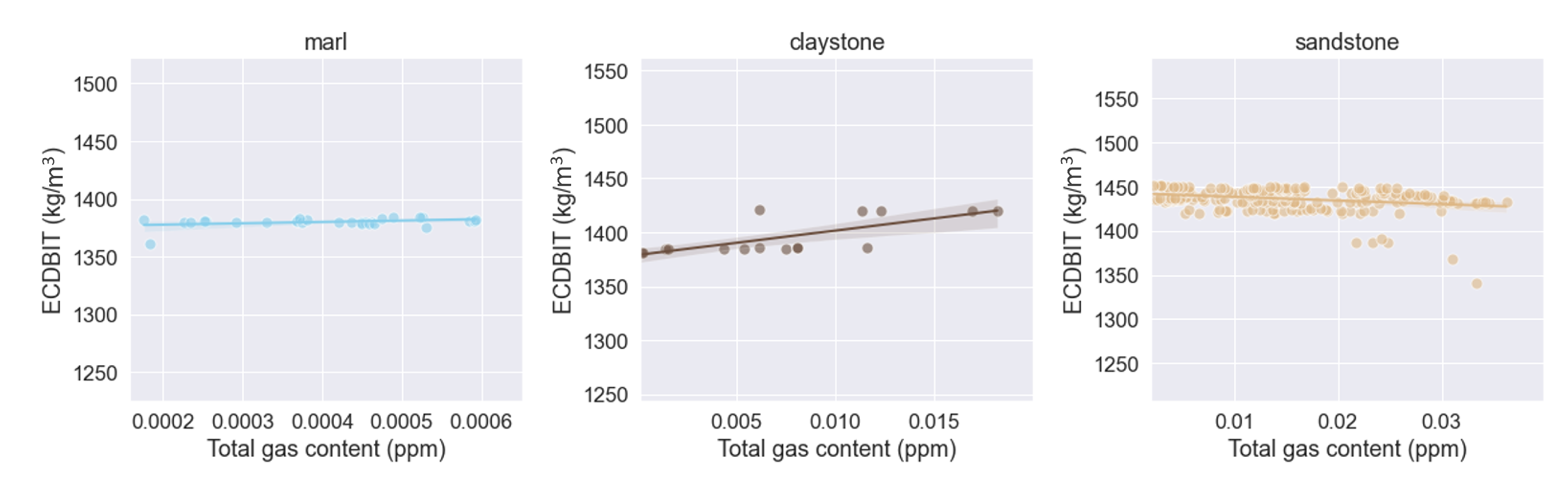
Our attention then shifts to Figure 13, which illustrates the relationship between total gas content (TOTGAS) and effective circulation density on the bit (ECDBIT) across different lithologies: marl, claystone, and sandstone via scatter plots. The ECDBIT represents the pressure exerted by the drilling fluid at the bit, which can affect drilling efficiency. The plots reveal varying patterns across lithologies. In the case of marl, a weak negative correlation is observed, suggesting that as gas content increases, the pressure exerted by the drilling fluid decreases. This could be attributed to the high clay content in marl, which swells in the presence of water and may restrict fluid flow. For claystone, a slight positive correlation is observed, which could indicate that the denser and less permeable nature of this lithology requires increased drilling fluid pressure to extract gas. Lastly, for sandstone, the correlation appears to be quite weak, possibly due to its high porosity and permeability allowing gas to flow more freely without significantly affecting the pressure of the drilling fluid. However, further detailed analysis would be required to confirm these interpretations and understand the underlying mechanisms.

4. Results

We utilized several machine-learning classifiers, namely random forest, gradient boost, LinearSVC, AdaBoost, and KNeighbors, for the dataset classification. These models were evaluated on their accuracy, quantified as the ratio of correct predictions to the total dataset size. To optimize the performance of each model, a thorough hyperparameter tuning was carried out using grid search. This process involved systematically searching through a predefined set of hyperparameter values, evaluating the models on a cross-validated subset of the training data, and selecting the combination that yielded the best performance [52]. The specific hyperparameter values used and the ones that demonstrated the best results for each classifier are detailed in

Table A2. Key hyperparameters considered for each ML model.

Model Name	Hyperparameter	Value	Definition
Random Forest	n_estimators	100	Number of trees in the forest
	criterion	‘gini’	Function to measure split quality
	max_depth	None	Maximum depth of tree
	max_features	‘sqrt’	Number of features to consider
	bootstrap	True	Whether bootstrap samples are used
	oob_score	False	Whether to use out-of-bag samples
Gradient Boost	n_estimators	100	Number of boosting stages
	learning_rate	0.1	Shrinks the contribution of each tree
	loss	‘log_loss’	Loss function to optimize
	max_depth	3	Maximum depth of tree
	criterion	‘friedman_mse’	Function to measure split quality
	subsample	1.0	Fraction of samples used for fitting
LinearSVC	C	1.0	Regularization parameter
	penalty	‘l1’	Used to specify the norm
	dual	False	Dual or primal formulation
	fit_intercept	True	Whether to compute the intercept
	loss	‘squared_hinge’	Specifies the loss function
AdaBoost	n_estimators	50	Number of weak learners
	learning_rate	1.0	Weight applied to each classifier
	algorithm	‘SAMME.R’	Boosting algorithm
KNeighbors	n_neighbors	3	Number of neighbors to use
	weights	‘uniform’	Weight function used in prediction
	algorithm	‘auto’	Algorithm to compute nearest neighbors
	metric	‘minkowski’	Distance metric for the tree

in Appendix B.

4.1. Classifiers Performance

The evaluation of the machine-learning models was performed with 65 samples from each class.The confusion matrices for each model, presented in

Table 3. True predictions of ML models for different lithology classes.

	Random Forest	Gradient Boost	LinearSVC	KNeighbors	AdaBoost
Claystone	60/65	35/65	32/65	44/65	35/65
Marl	65/65	65/65	65/65	65/65	0/65
Sandstone	65/65	64/65	63/65	61/65	64/65

, highlight random forest’s superior predictive capability. Although all models perfectly identified marl, random forest excelled in predicting claystone and sandstone. Conversely, AdaBoost faced challenges with marl.

The random forest classifier also emerged as the top-performing model with an accuracy of 96%, whereas the AdaBoost model registered the lowest accuracy of 89% (see Figure 14).

4.2. Random Forest Classifier Implementation and Evaluation

For the implementation of the random forest classifier, the dataset was partitioned into feature variables (X) and the target variable (Y), using a 70:30 train-test split ratio which led to 65 samples per class being used in the confusion matrix, as 30% of 219 is 65. Moreover, the total number of samples in the balanced dataset became 195, representing the sum of 65 samples for each of the three lithology classes. Feature normalization was ensured using the StandardScaler. To evaluate the model’s performance, a Repeated Stratified K-Fold Cross-Validation (CV) was applied with 10 splits and three repetitions [53].

The random forest classifier demonstrated an impressive accuracy of 96%, precision of 98%, and recall of 86% (see

Table 4. Metrics for the random forest classifier.

Metrics	Scores
Mean Accuracy	0.9564
Mean Precision	0.8420
Mean Recall	0.8608
Precision	0.9795

).

4.3. Model Evaluation

The confusion matrix of the random forest classifier model revealed a successful prediction of 61 claystone samples, 59 marl samples, and 65 sandstone samples out of a total of 65 samples for each (see Figure 15).

In our analysis, the random forest classifier demonstrated a robust performance in predicting three lithology types: claystone, marl, and sandstone. For the claystone class, the model achieved a precision of 91%, a recall of 94%, and an F1-score of 92%. In predicting the marl class, the model attained a precision of 0.97, a recall of 91%, and an F1-score of 0.94. The model showcased nearly perfect performance in predicting sandstone, achieving a precision of 97%, a recall of 100%, and an F1-score of 98%. The overall model accuracy was 95%, indicating that 95% of all predictions made by the model were correct. Furthermore, both the macro and weighted averages for precision, recall, and F1-score were 95%, indicating that the model performed consistently across all classes (see

Table 5. Classification report.

	Precision	Recall	F1-Score	Support
Claystone	0.91	0.94	0.92	65
Marl	0.97	0.91	0.94	65
Sandstone	0.97	1.00	0.98	65
Accuracy			0.95	195
Macro Avg	0.95	0.95	0.95	195
Weighted Avg	0.95	0.95	0.95	195

).

A bar plot representing feature importance was utilized to gain insights into the contribution of individual features to the random forest model. The analysis revealed that ‘TOTGAS‘ had the highest importance, whereas ‘WOB‘ had the lowest significance in the model construction (see Figure 16).

5. Results Summary

After building our model with well 1 data as the foundation, we meticulously evaluated its performance within this same dataset. The assessment involved comparing predicted and actual lithology results, revealing the model’s impressive accuracy in capturing lithological patterns (see Figure 17). The model demonstrated success rates of 100% for sandstone, 88% for claystone, and 96% for marl, yielding an overall success rate of 99%. These results reflect the model’s capability to learn meaningful relationships from the provided drilling parameters and effectively predict the majority of lithologies present in well 1.

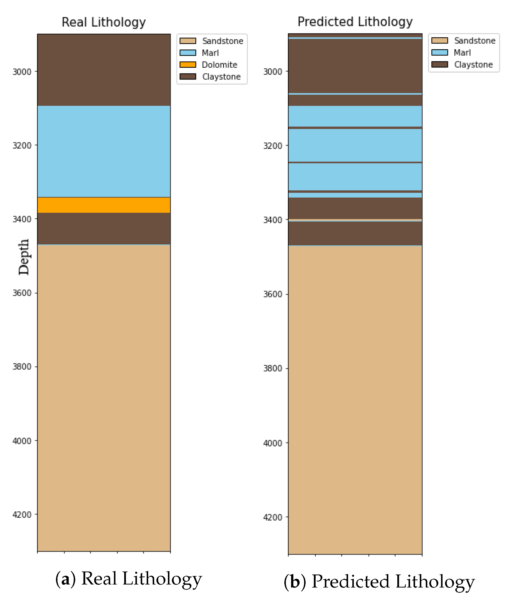
Expanding on the promising results achieved, the model’s adaptability was then put to the test through a comprehensive blind assessment. Well 2 was chosen as an entirely novel dataset, unassociated with the model’s training. This strategic selection aimed to evaluate the model’s generalization capacity. The model achieved success rates of 100% for sandstone, 87% for claystone, and 94% for marl in well 2. However, when considering Dolomite, which the model was not trained on, its prediction success was 0%. Notably, if well 2 did not encompass the Dolomite lithology, the overall success rate would have stood at 93%. Given its presence, the overall success rate was adjusted to 70% (refer to Figure 18).

The success rate for each lithology is computed as:

$$\mathrm{Success}\mathrm{Rate}=\frac{\mathrm{Number}\mathrm{of}\mathrm{Correct}\mathrm{Predictions}\mathrm{for}\mathrm{Lithology}}{\mathrm{Total}\mathrm{Number}\mathrm{of}\mathrm{True}\mathrm{Instances}\mathrm{of}\mathrm{Lithology}}$$

where n represents the number of lithologies.

Model Deployment

Once the model was trained and evaluated, the next crucial step was deploying it for practical use. The primary objective was to predict lithology types using nine drilling parameters as inputs and make them accessible through a user-friendly website or mobile application.Ensuring consistent performance and accuracy over time required a well-planned monitoring and maintenance strategy.

The deployment process involved the following steps:

• Model Serialization: the trained model was serialized using the pickle library in Python, saving it as a binary file.
• Web Framework: the Flask web framework in Python was employed to create a responsive web application capable of handling HTTP requests and responses (see Figure 19).
• Model Loading: during the application’s initialization, the serialized model was loaded into the web application’s memory for efficient usage.
• Prediction Endpoint: an endpoint was set up in the web application to receive input data in JSON format and return predictions in the same format.
• Deployment: the web application was successfully deployed on Sttreamlit web server, making it accessible for users.

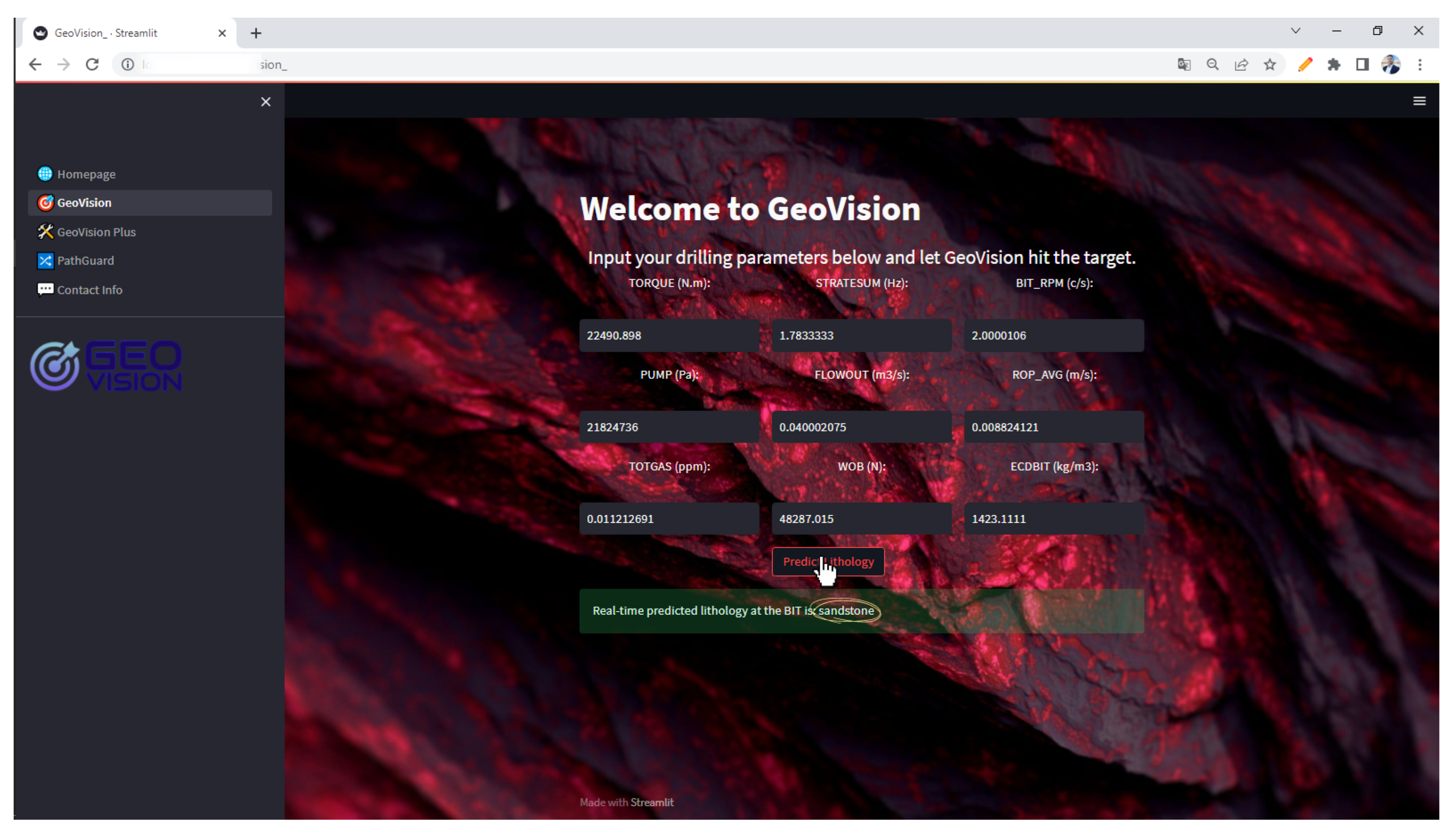
The GeoVision web app showcases a user-friendly interface with its intuitive design where users can easily input drilling parameters and promptly receive accurate lithology predictions as Figure 19 exemplifies its successful real-time lithology prediction, precisely identifying sandstone at the drill bit. These figures demonstrate the app’s ease of use and its potential as a tool for geological analysis and decision-making processes.

6. Discussion

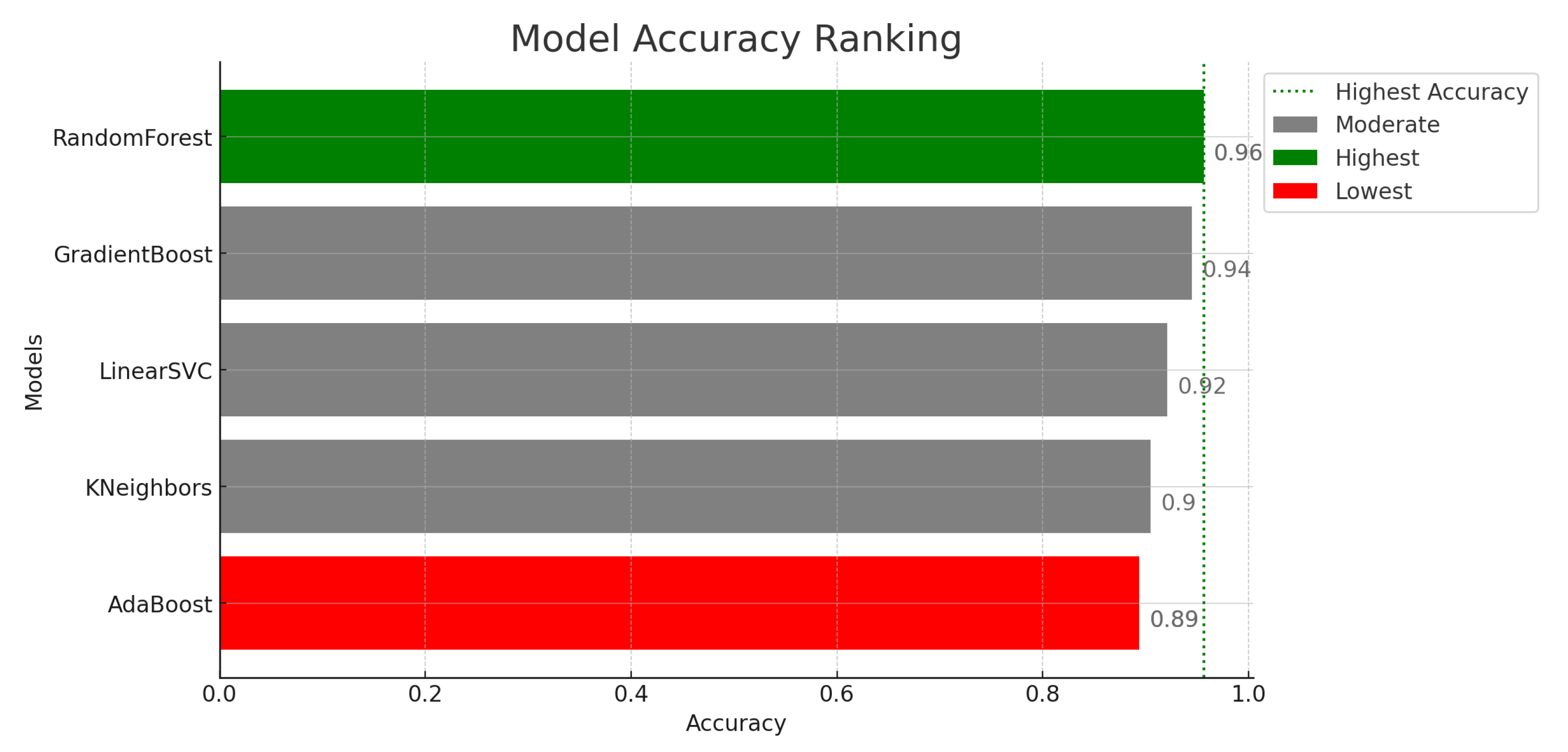
Our investigation into lithology prediction using machine-learning classifiers yielded valuable insights into the performance and practicality of different models. Among the classifiers tested, the random forest model emerged as the most accurate, boasting an impressive 96% accuracy rate. This high level of accuracy can be attributed to the ensemble approach of the random forest algorithm, which unifies multiple decision trees to make predictions.

This ensemble strategy enables it to grasp intricate relationships and interactions between drilling parameters and lithology types, making it well-suited for our prediction task. Notably, the work of Sun et al. (2019) and the conclusions drawn by Fernandez Delgado et al. (2014) also highlight the efficacy of the random forest classifier, reinforcing its suitability for lithology identification tasks [54,55].

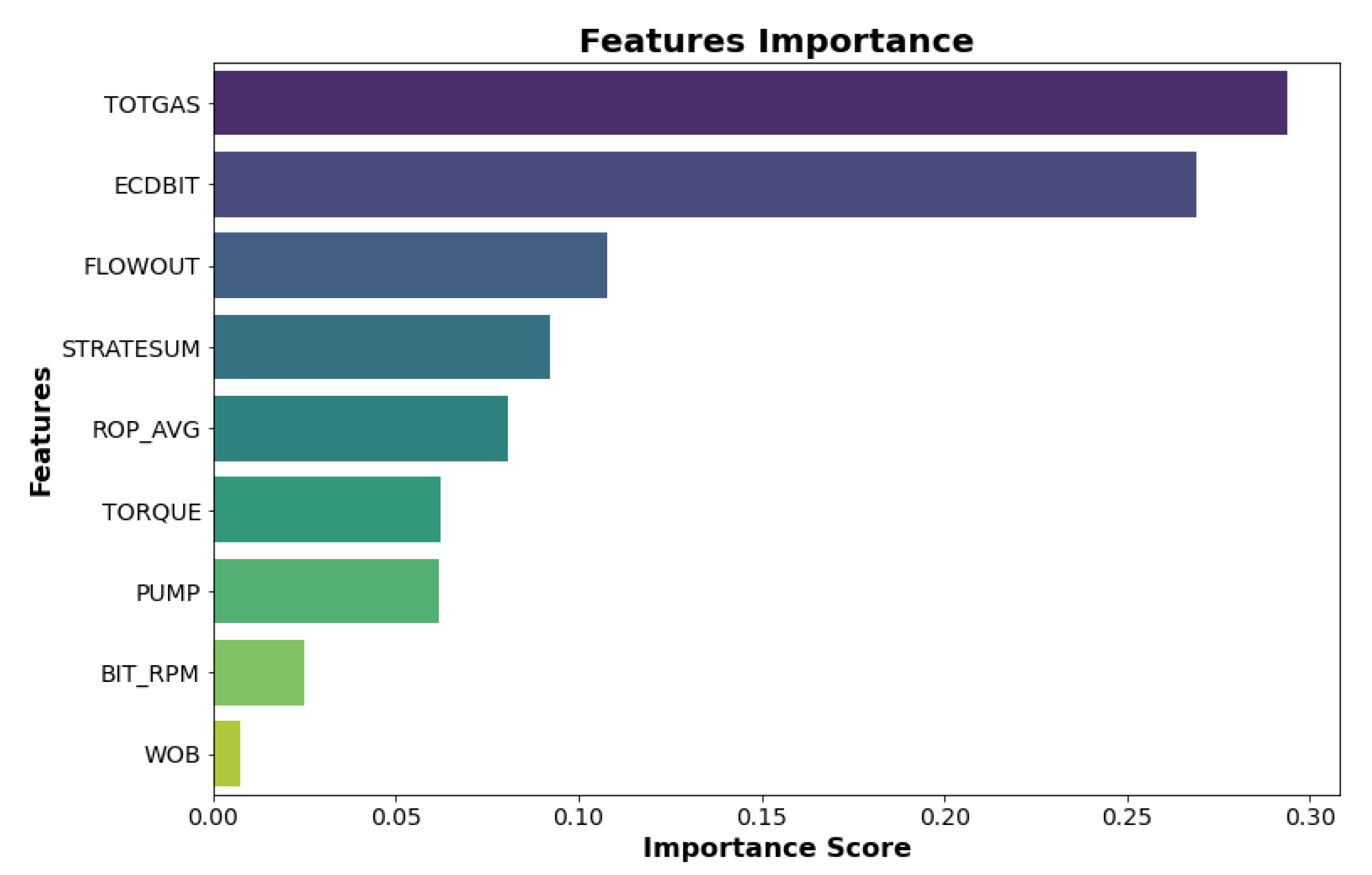
An essential element of our data analysis is the feature importance bar plot, which sheds light on the factors significantly influencing the lithology prediction model. These importance values are data-driven, yet they hold physical significance. Notably, the parameter representing total gas content (‘TOTGAS’) ranks as the most crucial feature, as variations in gas concentrations often serve as key indicators of different rock types and geological formations. Another influential factor is ‘ECDBIT’, characterizing effective circulation density on the bit, impacting drilling performance and efficiency, making it vital for distinguishing between lithologies. Additionally, the ‘FLOWOUT’ parameter, reflecting outgoing mud flow, holds significant importance in conveying information about subsurface formations, aiding in identifying lithological characteristics. Moreover, the ‘ROP’ (rate of penetration) parameter, representing average drilling speed, becomes essential in recognizing lithological transitions due to variations in drilling resistance. Understanding the physical significance of these influential parameters enhances our lithology prediction model and offers valuable insights for geological investigations and resource exploration.

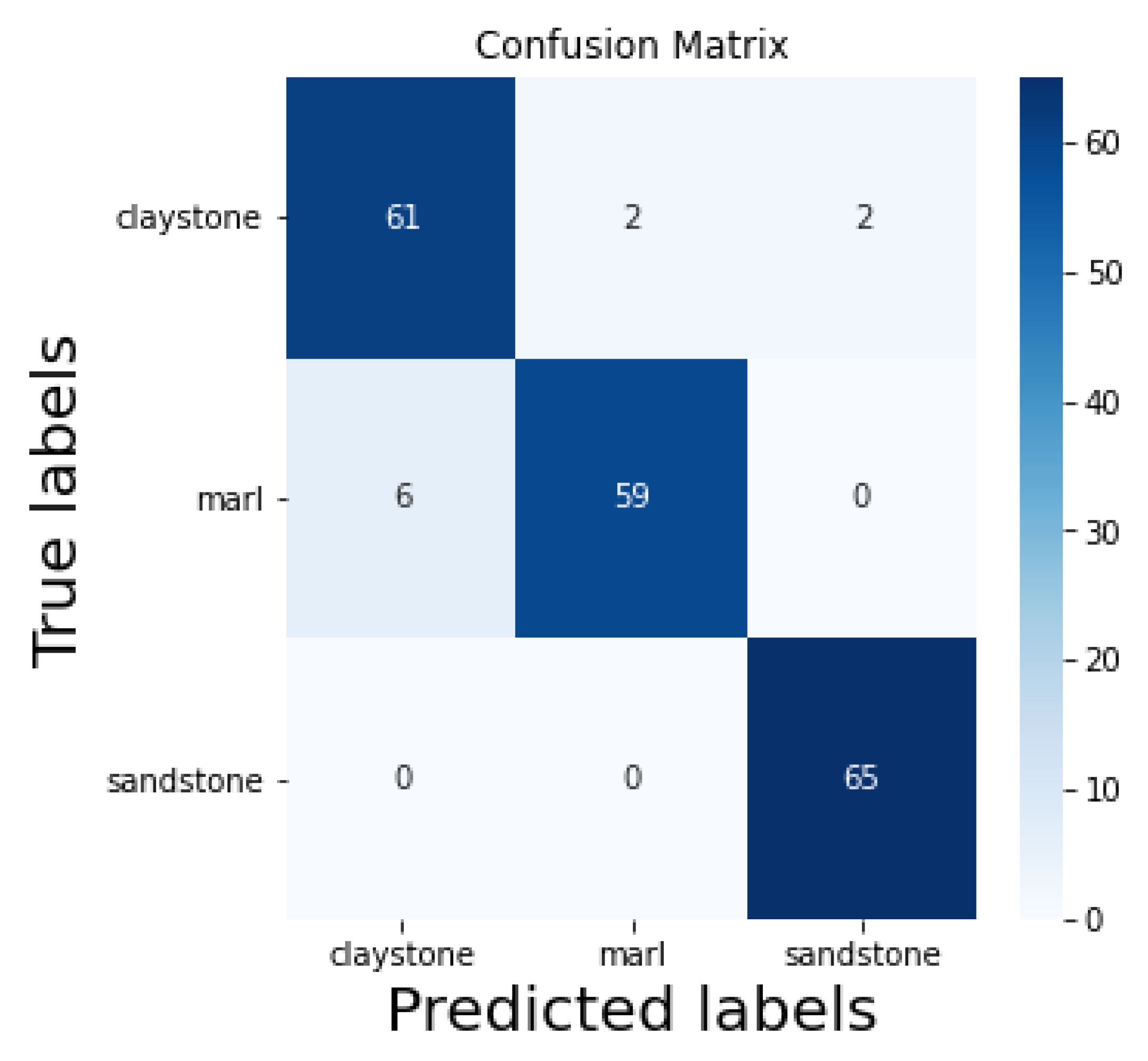
The random forest classifier demonstrated impressive performance in predicting lithology types, showcasing its ability to learn and generalize from the training data. With an accuracy of 95%, the model correctly classified the majority of lithologies, indicating the efficacy of the chosen features and the robustness of the random forest algorithm in capturing complex relationships. High precision values of 91% for claystone and 97% for both marl and sandstone highlight the model’s proficiency in accurately identifying instances of each lithology class. The 100% recall for sandstone suggests that the model successfully identified all samples of this class, whereas the slightly lower recall values for claystone (94%) and marl (91%) indicate some misclassifications. The confusion matrix further supports the model’s performance, showing successful predictions of 61 claystone, 59 marl, and 65 sandstone samples out of a total of 65 for each class.

Moreover, the random forest model exhibited robust generalization capabilities, performing well on well 1 data, which were used for model training, as well as on well 2 data, which it had never encountered before. This ability to generalize indicates that the model effectively learned meaningful patterns and features from the training data and applied this knowledge to accurately predict lithology in new wells. However, the model faced challenges in identifying dolomites in well 2, which can be attributed to the limited representation of dolomite samples in the training data. To overcome this limitation, future research can focus on collecting more data for rare lithologies to improve the model’s performance on such classes.

7. Conclusions

In this research, we present a machine learning-based approach to real-time lithology prediction using drilling data. The proposed methodology uses a random forest classifier to effectively differentiate claystone, marl, and sandstone, achieving a remarkable accuracy of 96%. Instead of relying solely on the traditional metric of rate of penetration (ROP) for lithology prediction, our model exploits the intricate relationships between a wider range of drilling data features, notably rate of penetration, total gas content, and torque.

Despite acknowledging some challenges in identifying rare lithologies, our research marks significant progress in immediate subsurface analysis. Crucially, this methodology, through real-time lithology insights during drilling operations, has the potential to significantly enhance geosteering capabilities, a vital aspect for maintaining the optimal well trajectory within the pay zone. The robustness of our results, underscored by consistent precision and recall values around 95%, validates the efficacy of our approach.

In conclusion, as we persist in refining our models and gathering data, we foresee major advancements in subsurface analysis. For example, this research paves the way for the development of ‘looking ahead of the bit’ projects which, by utilizing extensive datasets, could predict lithology ahead of the bit and extend the reach of our real-time insights. Furthermore, enhancements to our Geovision web application, like incorporating a dedicated section for streamlined, diverse data visualization features could make the app more user-friendly and insightful.