
Pressure Anomalies Beneath Solitary Waves with Constant Vorticity


Abstract
1. Introduction
2. Governing Equations
3. Conformal Mapping and the Numerical Method
3.1. Conformal Mapping
3.2. Numerical Method
4. Results
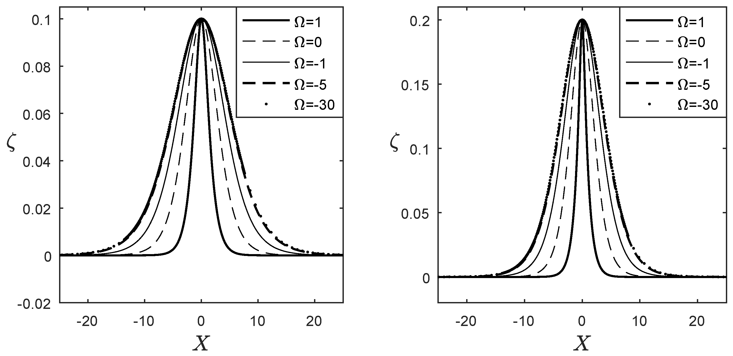
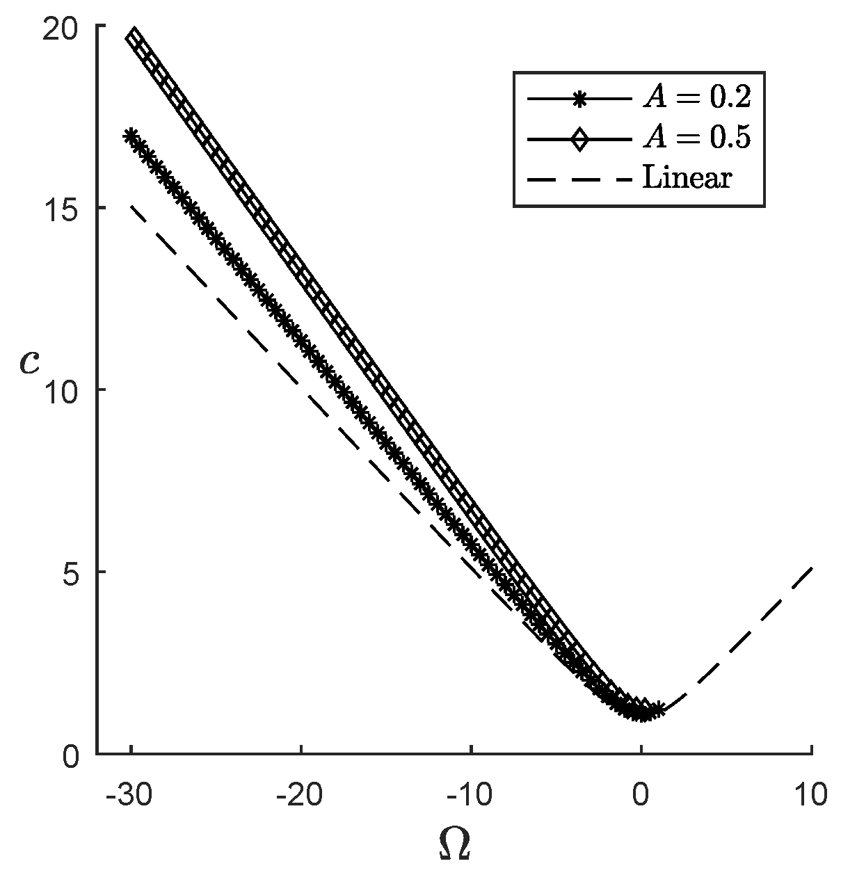
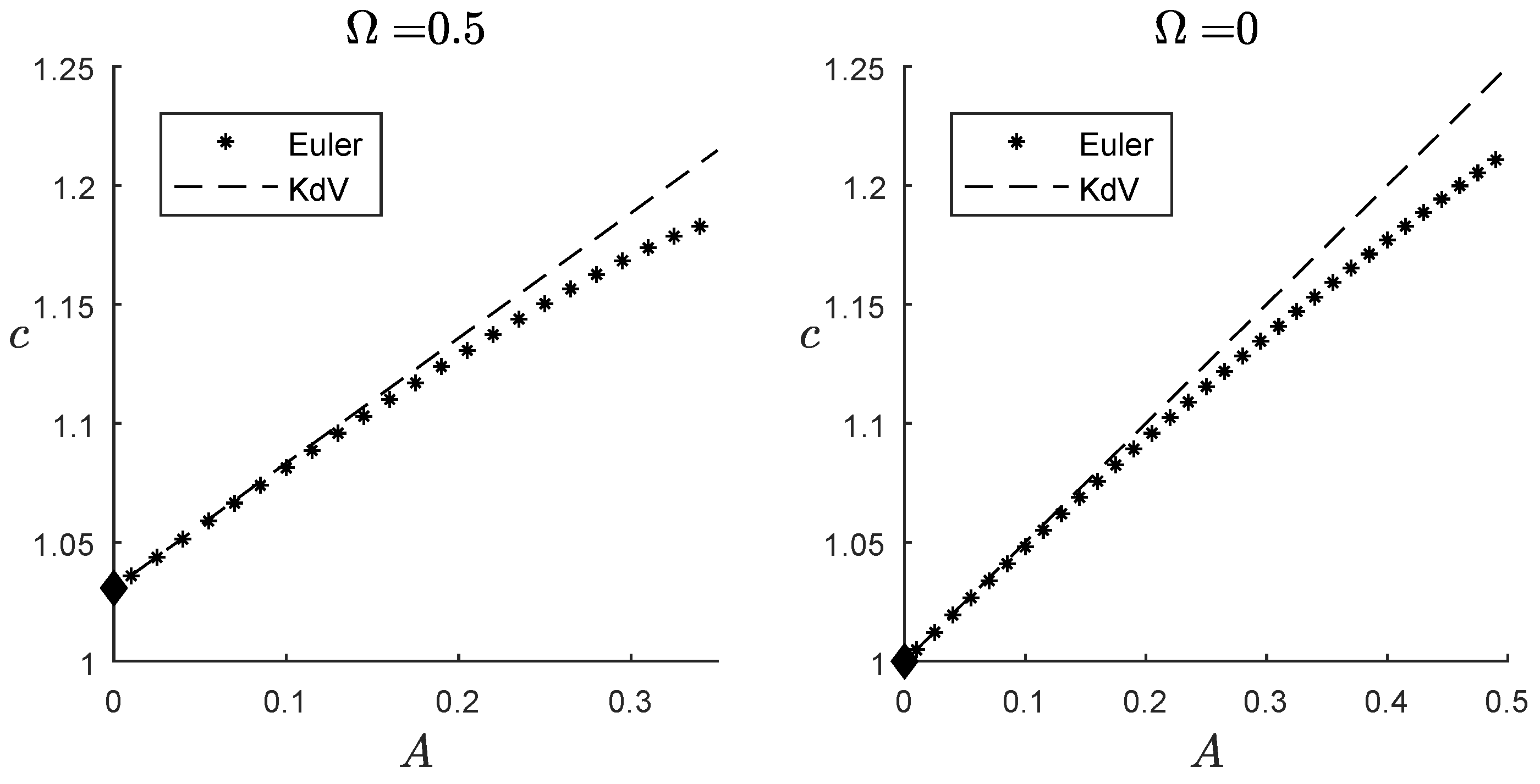
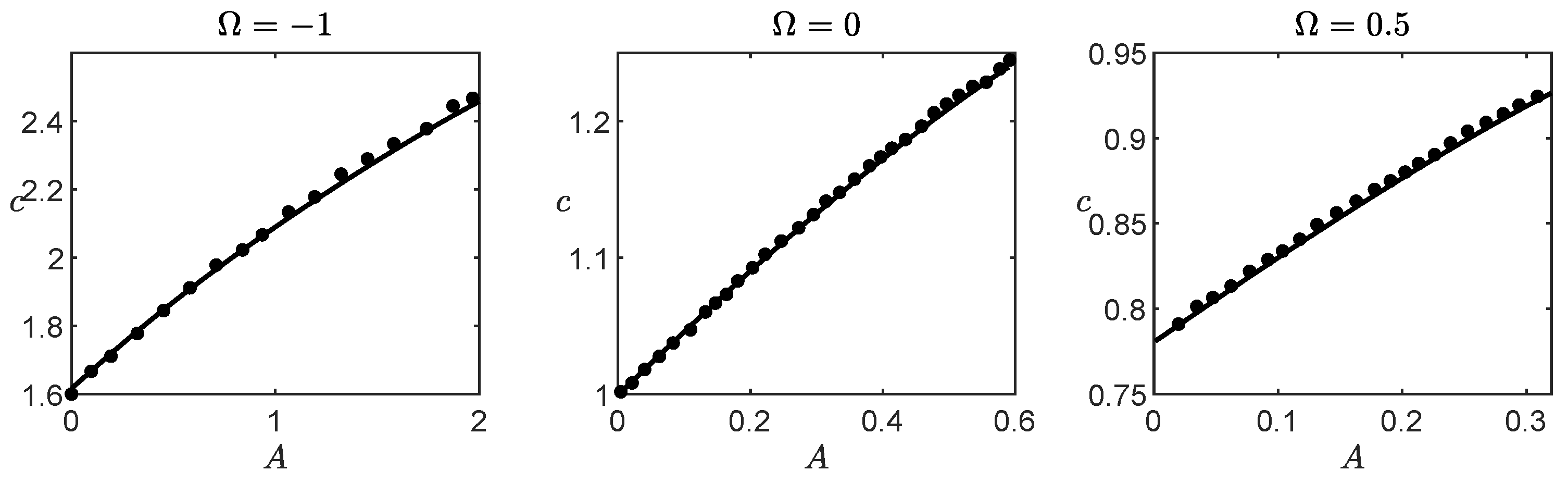
4.1. Steady Waves
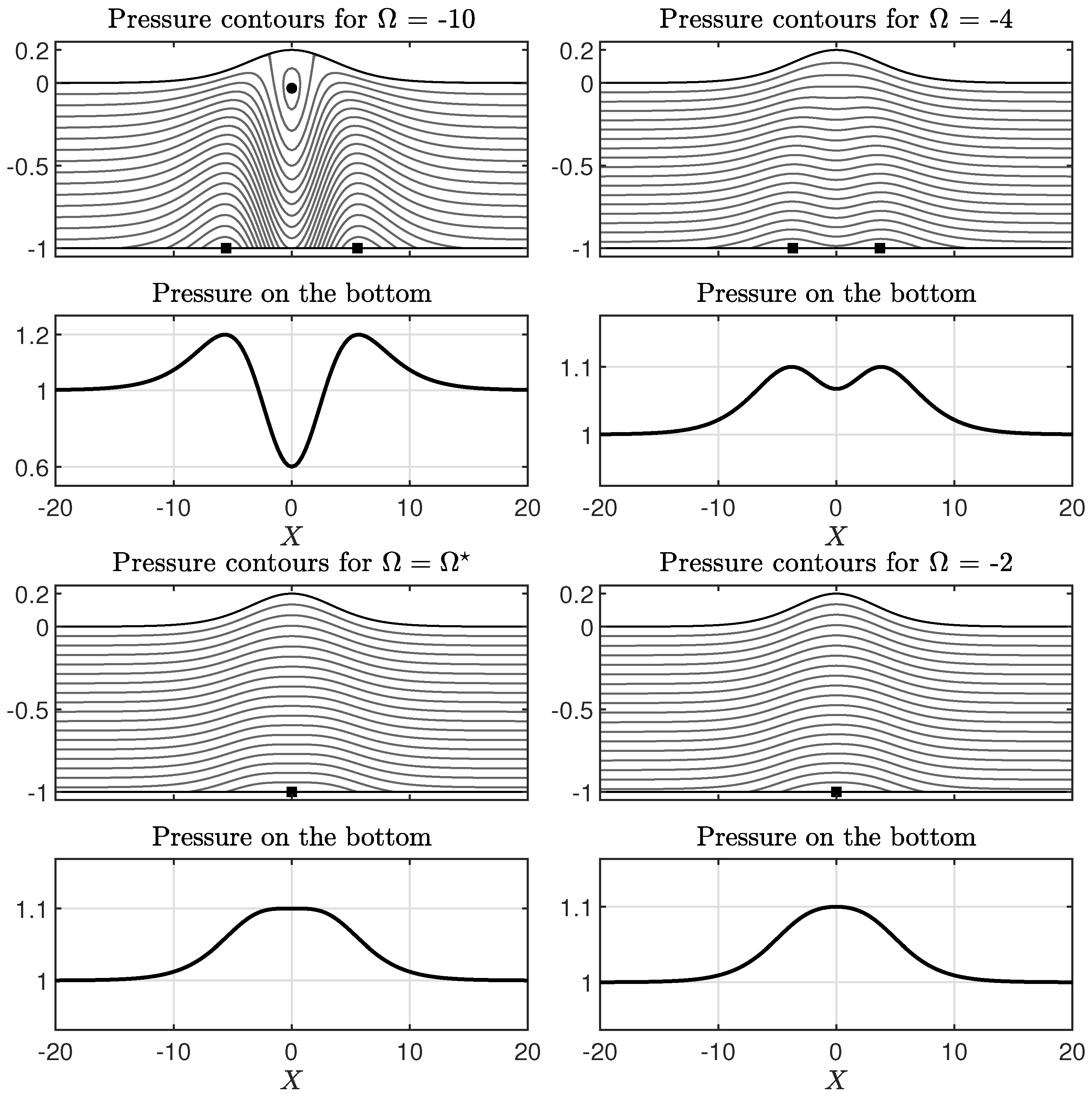
4.2. Pressure in the Bulk of the Fluid
5. Conclusions
Author Contributions
Funding
Institutional Review Board Statement
Informed Consent Statement
Data Availability Statement
Acknowledgments
Conflicts of Interest
Abbreviations
| Symbol | Meaning |
| B | Bernoulli constant |
| c | Wave speed |
| The periodic Hilbert transform on a strip of width D | |
| D | Width of strip that corresponds to the canonical domain |
| F | Froude number |
| L | Length of the canonical domain |
| p | pressure in fluid body |
| Coordinate system in the canonical domain | |
| Conformal mapping that applies a strip of width D in the physical domain. | |
| Free surface wave profile written in terms of the conformal mapping | |
| Dimensionless vorticity | |
| Laboratory frame of reference | |
| Free surface wave profile in the moving frame and | |
| Velocity potential for the irrotational part of the velocity field | |
| Harmonic conjugate function of | |
| Potential written in the coordinate system | |
| Function written in the coordinate system | |
| Potential evaluated at | |
| Function evaluated at |
Appendix A. Resolution Study

| 0 | |||
| −1 | |||
| 1 | |||

Appendix B. The Free Surface Wave in the Canonical Coordinate System
References
- Dalrymple, R.A. Water Wave Models and Wave Forces with Shear Currents; Technical Report No. 20; Coastal and Oceanographic Engineering Laboratory, University of Florida: Gainesville, FL, USA, 1973. [Google Scholar]
- Teles Da Silva, A.F.; Peregrine, D.H. Steep, steady surface waves on water of finite depth with constant vorticity. J. Fluid Mech. 1988, 195, 281–302. [Google Scholar] [CrossRef]
- Vanden-Broeck, J.-M. Periodic waves with constant vorticity in water of infinite depth. IMA J. Appl. Maths 1996, 56, 207–217. [Google Scholar] [CrossRef]
- Vanden-Broeck, J.-M. Steep solitary waves in water of finite depth with constant vorticity. J. Fluid Mech. 1994, 274, 339–348. [Google Scholar] [CrossRef]
- Dyachenko, S.A.; Hur, V.M. Stokes waves with constant vorticity: Folds, gaps and fluid bubbles. J. Fluid Mech. 2019, 878, 502–521. [Google Scholar] [CrossRef]
- Dyachenko, S.A.; Hur, V.M. Stokes waves with constant vorticity: I. Numerical computation. Stud. Appl. Maths 2019, 142, 162–189. [Google Scholar] [CrossRef]
- Constantin, A.; Strauss, W.; Vărvărucă, E. Global bifurcation of steady gravity water waves with critical layers. Acta Math. 2016, 217, 195–262. [Google Scholar] [CrossRef]
- Hur, V.M.; Wheeler, M. Overhanging and touching waves in constant vorticity flows. J. Differ. Equations 2022, 338, 572–590. [Google Scholar] [CrossRef]
- Haziot, S.V.; Wheeler, M. Large-amplitude steady solitary water waves with constant vorticity. arXiv 2021, arXiv:2110.04901. [Google Scholar] [CrossRef]
- Varvaruca, E. Singularities of Bernoulli free boundaries. Commun. Partial Differ. Equations 2006, 31, 1451–1477. [Google Scholar]
- Flamarion, M.V.; Ribeiro, R., Jr. Solitary Waves on Flows with an Exponentially Sheared Current and Stagnation Points. Q. J. Mech. Appl. Math. 2023, 76, 79–91. [Google Scholar] [CrossRef]
- Ige, O.E.; Kalisch, H. Particle trajectories in a weakly nonlinear long-wave model on a shear flow. Appl. Numer. Math. 2023, in press. [Google Scholar] [CrossRef]
- Constantin, A.; Strauss, W. Pressure beneath a Stokes wave. Comm. Pure. Appl. Math. 2010, 63, 533–557. [Google Scholar] [CrossRef]
- Ali, A.; Kalisch, H. Reconstruction of the pressure in long-wave models with constant vorticity. Eur. J. Mech. B Fluids 2013, 37, 187–194. [Google Scholar] [CrossRef]
- Ribeiro, R., Jr.; Milewski, P.A.; Nachbin, A. Flow structure beneath rotational water waves with stagnation points. J. Fluid. Mech. 2017, 812, 792–814. [Google Scholar] [CrossRef]
- Strauss, W.A.; Wheeler, M. Bound on the slope of steady water waves with favorable vorticity. Arch. Rat. Mech. Anal. 2016, 222, 1555–1580. [Google Scholar] [CrossRef]
- Vasan, V.; Oliveras, K. Pressure beneath a travelling wave with constant vorticity. DSDC-A 2014, 34, 3219–3239. [Google Scholar]
- Kozlov, V.; Kuznetsov, N.; Lokharu, E. Solitary waves on constant vorticity flows with an interior stagnation point. J. Fluid. Mech. 2020, 904, A4. [Google Scholar] [CrossRef]
- Dyachenko, A.; Zakharov, V.; Kuznetsov, E. Nonlinear dynamics of the free surface of an ideal fluid. Plasma Phys. 1996, 22, 916–928. [Google Scholar]
- Choi, W. Strongly nonlinear long gravity waves in uniform shear flows. Phys. Rev. E 2003, 68, 026305. [Google Scholar] [CrossRef]
- Milewski, P.; Vanden-Broeck, J.; Wang, Z. Dynamics of steep two-dimensional gravity-capillary solitary waves. J. Fluid Mech. 2010, 664, 466–477. [Google Scholar] [CrossRef]
- Flamarion, M.V.; Ribeiro, R., Jr. An iterative method to compute conformal mappings and their inverses in the context of water waves over topographies. Int. J. Numer. Methods Fluids 2021, 93, 3304–3311. [Google Scholar] [CrossRef]
- Trefethen, L.N. Spectral Methods in MATLAB; SIAM: Philadelphia, PA, USA, 2001. [Google Scholar]
- Ko, J.; Strauss, W. Large-amplitude steady rotational water waves. Eur. J. Mech. 2008, 27, 96–109. [Google Scholar] [CrossRef]
- Guan, X. Particle trajectories under interactions between solitary waves and a linear shear current. Theor. Appl. Mech. Lett. 2020, 10, 125–131. [Google Scholar] [CrossRef]


Disclaimer/Publisher’s Note: The statements, opinions and data contained in all publications are solely those of the individual author(s) and contributor(s) and not of MDPI and/or the editor(s). MDPI and/or the editor(s) disclaim responsibility for any injury to people or property resulting from any ideas, methods, instructions or products referred to in the content. |
© 2023 by the authors. Licensee MDPI, Basel, Switzerland. This article is an open access article distributed under the terms and conditions of the Creative Commons Attribution (CC BY) license (https://creativecommons.org/licenses/by/4.0/).
Share and Cite
Flamarion, M.V.; Castro, E.M.; Ribeiro-Jr, R. Pressure Anomalies Beneath Solitary Waves with Constant Vorticity. Eng 2023, 4, 1306-1319. https://doi.org/10.3390/eng4020076
Flamarion MV, Castro EM, Ribeiro-Jr R. Pressure Anomalies Beneath Solitary Waves with Constant Vorticity. Eng. 2023; 4(2):1306-1319. https://doi.org/10.3390/eng4020076
Chicago/Turabian StyleFlamarion, Marcelo V., Eduardo M. Castro, and Roberto Ribeiro-Jr. 2023. "Pressure Anomalies Beneath Solitary Waves with Constant Vorticity" Eng 4, no. 2: 1306-1319. https://doi.org/10.3390/eng4020076
APA StyleFlamarion, M. V., Castro, E. M., & Ribeiro-Jr, R. (2023). Pressure Anomalies Beneath Solitary Waves with Constant Vorticity. Eng, 4(2), 1306-1319. https://doi.org/10.3390/eng4020076