Abstract
The traditional means of monitoring the health of industrial systems involves the use of vibration and performance monitoring techniques amongst others. In these approaches, contact-type sensors, such as accelerometer, proximity probe, pressure transducer and temperature transducer, are installed on the machine to monitor its operational health parameters. However, these methods fall short when additional sensors cannot be installed on the machine due to cost, space constraint or sensor reliability concerns. On the other hand, the use of acoustic-based monitoring technique provides an improved alternative, as acoustic sensors (e.g., microphones) can be implemented quickly and cheaply in various scenarios and do not require physical contact with the machine. The collected acoustic signals contain relevant operating health information about the machine; yet they can be sensitive to background noise and changes in machine operating condition. These challenges are being addressed from the industrial applicability perspective for acoustic-based machine condition monitoring. This paper presents the development in methodology for acoustic-based fault diagnostic techniques and highlights the challenges encountered when analyzing sound for machine condition monitoring.
1. Introduction
Unplanned interruption of industrial processes can result in serious financial losses; as such, it becomes of significant relevance to prevent unplanned shutdowns of machinery. The monitoring and diagnosis of the current health state of the machine is crucial in achieving this.
The conventional approach of machine health monitoring involves the use of vibration and other performance monitoring techniques. In these circumstances, sensors such as accelerometer, proximity probe, pressure transducer and temperature transducer are installed on the machine to monitor its health state. However, these methods are of an intrusive nature, requiring physical modification of the machine for their installation. Alternatively, the use of acoustic-based monitoring provides an improved approach which is non-intrusive to the machine operation. Sound signals from a machine contains substantial relevant health information; however, acoustic signals in an industrial environment can be affected by background noise from neighbouring operating machineries; thus, posing a challenge during industrial condition monitoring.
The analysis of sound has been successful in speech and music recognition, especially for creating smart and interactive technologies. Within this context, there exist several large-scale acoustic datasets such as Audio Set [1] and widely available pre-trained deep learning models for audio event detection and classification such as: OpenL3 [2,3], PANNs [4] and VGGish [5]. However, within the context of machine condition monitoring and fault diagnostics, these is a nascent problem for the detection and classification of acoustic scenes and events [6,7,8].
This paper presents the development in methodology for acoustic-based diagnostic techniques and explores the challenges encountered when analysing sound for machine condition monitoring.
2. Methods—Acoustic-Based Machine Condition Monitoring
2.1. Detection of Anomalous Sound
The goal of anomalous sound detection is to determine if the sound produced by a machine during operation typifies a normal or an abnormal operating state. The ability to detect such automatically is fundamental to machine fault diagnostics using data driven techniques. However, the challenge with this task is that sound produced from anomalous state operation of the machine is rare and varies in nature, hence presenting difficulty in collecting training dataset of such observed abnormal machine operating state. Furthermore, in actual industrial applications, it would be costly and damaging to consider running machines with implanted faults for the sake of data collection. Therefore, the traditional approaches which may be initially apparent such as framing the problem as a two-class classification problem becomes impractical.
In addressing the anomalous sound detection problem, consideration must be given to the fact that only training dataset of the machine running in its normal state would be available. As such, this forms the context within which the problem should be considered. Any such technique would have to learn the normal behaviour of the machine based on this available training dataset.
In furtherance of actualizing anomalous machine sound detection for industrial environment, saw the birth of the Detection and Classification of Acoustic Scenes and Events (DCASE) challenge task “Unsupervised Detection of Anomalous Sounds for Machine Condition Monitoring” in 2020. With the provision of a comprehensive acoustic training dataset combining ToyADMOS [9] dataset and MIMII dataset [10], six categories of machines (i.e., toy and real) of toy car, toy conveyor, valve, pump, fan, and slide rail, operating both in normal and abnormal conditions were considered; researchers were expected to develop and benchmark techniques for detection of anomalous machine sounds. Since the inclusion of this task as part of the DCASE Challenge, over the subsequent years, the task has evolved to account for challenges such as: domain shifted conditions (i.e., accounting for changes in machine operating speed, load, and background noise) [11] and domain generalisation (i.e., invariant to changes in machine operating speed, load, and background noise) [12].
The challenge of machine anomaly detection is to find a boundary between normal and anomalous operating sound. In achieving this, the following methods have emerged.
2.1.1. Autoencoder-Based Anomaly Detection
An autoencoder is a neural network, trained to learn the output as an accurate reconstructed representation of the original input. As an unsupervised learning technique, it has been used by several studies for the detection of anomalous machine operating sound [7,8,9,10,13,14,15].
Autoencoder acts as a multi-layer neural network as shown in Figure 1, consisting of the following segments: encoder network, which accepts a high-dimensional input and transforms to a low-dimensional representation, decoder network, which accepts a latent low-dimensional input to reconstruct the original input, and at least a bottleneck stage within the network architecture. The presence of the bottleneck stage acts to compress the knowledge representation of the original input in order to learn the latent space representation. When the autoencoder is used for anomaly detection the goal during training is to minimize the reconstruction error between the input and the output using the normal machine operating sounds. Herein, the reconstruction error is used as the anomaly score. Anomalies are detected by thresholding the magnitude of the reconstruction error. Based on the application, this threshold could be set. Once an anomalous machine operating sound is provided to the system, it would yield a higher-than-normal reconstruction error, thereby flagging as a fault mode. Table 1 provides baseline autoencoder architecture parameters as applied for anomaly detection. Purohit et al. [10] implemented AE for anomaly detection based on acoustic dataset of malfunctioning industrial machines consisting of faulty valve, pump, fan, and slide rail. Although the dataset used MIMII [10] has been made publicly available, a key part of their work is the adopted architecture of their AE model. Purohit et al. [10] based the input layer on the log-Mel spectrogram. The Mel spectrogram is a spectrogram where frequencies have been transformed to the Mel scale. The Mel spectrogram provides a good correlation with human perception of sound, due to the Mel scale representing scale of pitches that humans would perceive to be equidistant from each other. As such, it not uncommon to find log-Mel spectrogram as performant input feature representation for acoustic event classification amongst others [16]. In [10], the log Mel spectrogram was determined for a frame size of 1024 acoustic time series data points, with a hop size of 512 and 64 Mel filter banks. This results in a log Mel spectrogram of size equal 64. This process was repeated for five consecutive frame sizes. The final input layer feature is formed by concatenating the log Mel spectrogram of five consecutive frames, resulting in an input feature vector size of 5 × 64 = 320. This is feed into an auto-encoder network with fully connected layers (FC) such as: encoder section—FC (input, 64, ReLU), FC (64, 64, ReLU), and FC (64, 8, ReLU) and decoder section—FC (8, 64, ReLU), FC (64, 64, ReLU) and FC (64, Output, none). Here, FC (x, y, z) translates fully connected layer with x input neurons, b output neuron, and z activation function such as rectified linear units (ReLU). The implemented AE model is trained for 50 epochs using Adam optimization approach. Similar approach can be adopted using the baseline AE topologies in Table 1.

Figure 1.
Schematic of an autoencoder [17].

Table 1.
Baseline auto encoder system architecture for anomaly detection.
2.1.2. Gaussian Mixture Model-Based Anomaly Detection
Gaussian Mixture Model (GMM) is an unsupervised probabilistic clustering model that assumes each data point belongs to a Gaussian distribution with unknown parameters. As an unsupervised learning technique, it has been used by several studies for the detection of anomalous machine operating sound [19,20,21].
GMM approach finds a mixture of multi-dimensional Gaussian probability distributions that most likely model the dataset. To achieve this, expectation-maximisation algorithm is used to estimate the parameters of the Gaussian distributions: mean, covariance matrix and mixing coefficients. Expectation-maximisation method is a two-step iterative process which aims to find the maximum likelihood estimates of the Gaussian mixture parameters. It alternates between the expectation step and the maximisation step. Within the expectation step, the responsibilities (which data point belongs to which cluster) are determined using the current estimate of the model parameters, while the maximisation step estimates the model parameters for maximizing the expected log-likelihood function. GMM for anomaly detection uses trained GMM model based on acoustic features as shown in Table 2 to predict the probability of each datapoint being part of one of the k Gaussian distribution clusters. An anomaly is detected by a data point having a probability lower than a threshold which could be either a percentage or a value threshold.
Table 2.
Baseline GMM acoustic features.
2.1.3. Outlier Exposure-Based Anomaly Detection
Outlier Exposure (OE) is an approach for improved anomaly detection in deep learning models [22]. Key in this method is the use of an out-of-distribution dataset, to fine tune a classifier model that enables it to learn heuristics that discriminate in-distribution data points from anomalies. The learned heuristics then has the capability to generalize to new distributions. The OE methodology, first proposed by [22], is achieved by adding a secondary loss to the regular loss for in-distribution training data, which is usually a cross-entropy loss or an error loss term. For classification models, the secondary loss is also a cross-entropy loss computed between the outlier logits and a uniform distribution.
The OE approach has already been applied in the domain of detecting anomalous machine operating sound using classifier models such as MobileNetV2 [11,12]. Herewith, MobileNetV2 [23] is trained to identify from which data segment within both in-distribution and out-of-distribution datasets the observed signal was generated (machine anomaly identification). The trained classifier then outputs the SoftMax value that is the predicted probability for each data segment. The anomaly score becomes the averaged negative logit of the predicted probabilities of the correct data segment. Table 3 shows baseline parameters for an OE approach using MobileNetV2 classifier model.
Table 3.
Baseline OE architecture based on MobileNetV2.
2.1.4. Signal Processing Methods
Acoustic signal processing methods are an adaptation from existing vibration-based approaches reliant on time, frequency, and time-frequency domain analysis of the signal.
Time domain analysis is performed on the acoustic signal time series representation through statistical analysis for calculating feature parameters such as mean, standard deviation, skewness, kurtosis, decibel, crest factor, beta distribution parameters, root mean square, maximum value, etc. These calculated statistical feature parameters from the acoustic signal are used to provide an overall indication of the current health condition of the machine. This approach, although simplistic, has been explored by various investigations for acoustic-based machine fault detection: e.g., Heng and Nor [24] evaluated the applicability of the statistical parameters such as crest factor, kurtosis, skewness, and beta distribution as fault indicators from acoustic signals for monitoring rolling element bearing defect.
For a machine operation under steady state conditions, frequency domain analysis techniques are commonly applied to examine the acoustic signals. Fast Fourier Transform (FFT), a computationally cheap technique to transform time-domain signals to the frequency domain, has been applied in acoustic-based condition monitoring of electric induction motors [25,26], engine intake air leak [27], among others. To capture nonlinear and nonstationary processes in machine operations, Ensemble Empirical Mode Decomposition (EEMD) method has been used [28]. EEMD simulates an adaptive filter, extracting underlying modes in the signal to decompose into a series of intrinsic mode functions (IMF) from high to low frequency content. Spectrum of IMFs has been adopted as a fault indicator for detecting incipient faults in wind turbine blades from acoustic signals [29].
Furthermore, time-frequency domain analysis, such as, short time Fourier transform and wavelet transform, are also powerful approaches for capturing nonstationary processes within machinery acoustic signals. Grebenik et al. [30] used consumer grade microphones and applied EMD and wavelet transform as diagnostic criteria for the acoustic fault diagnostics of transient current instability fault in DC electric motor. Spectral autocorrelation map of acoustic signals has been applied for detection of fault in belt conveyor idler [31]. EMD and wavelet analysis has been applied to extract features from acoustic signals produced by a diesel internal combustion engine for monitoring its combustion dynamics [32,33]. Anami and Pagi [34] used the chaincode of the pseudospectrum to analyse acoustic fault signals from a motorcycle for fault detection.
2.2. Classification of Anomalous Sound
The goal of classification of anomalous sound is to categorise a machine sound recording into one of the predefined fault classes that characterises the machine fault state.
Two main approaches have emerged for machine fault diagnostics based on acoustic signal. The first based on feature-based machine learning techniques and the second based on 2D acoustic representation deep learning approaches.
2.2.1. Feature-Based Machine Learning Methods
Feature-based machine learning methods can be broken into three stages. The first stage involves, extracting features from the machine condition acoustic signals. Features are important as fault descriptors are determined using statistical methods, fast Fourier transform, EEMD, or wavelet transform, etc. Extracted features are used to train a machine learning classifier such as Support Vector Machine (SVM), k-Nearest Neighbor (kNN), Random Forest (RF), logistic regression, naïve Bayes, Deep Neural Network (DNN), etc. The trained ML model is then used as a predictor for machine health state based on unknown machine condition acoustic signals.
This approach for machine fault detection based on acoustic inputs is presented in Figure 2. Although the system consists of several steps, the focus here would be in addressing the challenges in engineering feature extraction and for selecting appropriate classifier learning algorithm.

Figure 2.
Schematic of feature extraction-based technique for machine fault detection based on acoustic inputs.
- (1)
- Feature Extraction
An approach for acoustic signal representation is required, which is capable to differentiate normal and abnormal operating sound from machinery, utilising low-level features derived from the time domain, frequency domain and time-frequency domain of the acoustic signal. This is achieved as follows and summarized in Table 4:
- (a)
- Time domain-based feature extraction
Time domain features find their basis from descriptive statistical parameters derived from the acoustic signal time-series for representation of both healthy and faulty machine states and training various machine learning models. This approach has been adopted by several investigators [35] and relevant time-domain parameters summarized in Table 4.
- (b)
- Frequency domain-based feature extraction
Frequency domain features take their basis from the Fourier transform spectral transformation of the acoustic signal. Pasha et al. [36] used a band-power ratio as discriminant feature from acoustic signals to monitor air leaks in a sintering plant associated with pallet fault. Here, band-power ratio refers to the ratio of the spectral power within the fault frequency band to the spectral power of the entire signal spectrum. In [36], the feature extraction from a sound recording consisted of the band-power ratio performed repeatedly at fixed sampling window length (i.e., 1024 samples) within the fixed time duration/recording. Other potential parameters can be extracted from the frequency spectrum as demonstrated by [37] and listed in Table 4.
- (c)
- Time-frequency domain-based feature extraction
Time-frequency signal analysis refer to approaches that enable the simultaneous study of signals in both time and frequency domain. The time-frequency representations, such as STFT, wavelet transform, Hilbert-Huang transform, amongst others, provide useful parameters to characterise acoustic signals. Based on the work of [37], relevant time-frequency parameters are provided in Table 4.
Table 4.
Feature extraction parameters [37].
Table 4.
Feature extraction parameters [37].
| SN | Signal Analysis Domain | Features | Summary |
|---|---|---|---|
| 1 | Time Domain | Zero Crossing Rate | The rate of sign-changes along a signal within a frame length. |
| 2 | Frequency Domain | Short-time Energy | The sum of squares of the signal values normalised by frame length. |
| 3 | Frequency Domain | Entropy of Energy | Shannon entropy of the normalised energies within a frame length. |
| 4 | Frequency Domain | Spectral Centroid | The centre of mass of the spectrum of a frame. Determined by the weighted mean of the frequencies present within the spectrum of a frame length. |
| 5 | Frequency Domain | Spectral Spread | The second central moment of the spectrum of a frame length |
| 6 | Frequency Domain | Spectral Entropy | Shannon entropy of the normalised spectral energies within the spectrum of a frame length. |
| 7 | Frequency Domain | Spectral Flux | The squared difference between the normalised magnitudes of the spectra of the two successive frame length. |
| 8 | Frequency Domain | Spectral Roll-off | This is the frequency below which 90% of the spectral distribution for the frame is concentrated. |
| 9 | Frequency Domain | MFCC | Mel-Frequency Cepstrum Coefficient (MFCC) provide an effective representation of sound which closely mimics the sound perception of the human ear. MFCC are determined by taking the linear Discrete Cosine Transform (DCT) of the log power spectrum on the nonlinear Mel scale. |
| 10 | Frequency Domain | Chroma Vector | A representation of the spectrum projected onto 12 bins representing the 12 distinct semitones (or chroma) of the musical octave. |
| 11 | Frequency Domain | Chroma Deviation | Standard deviation of the chroma vector. |
| 12 | Frequency Domain | Band-power ratio | Normalised spectral peaks within fault frequency band |
- (2)
- Classifier Learning Algorithms
Classifier learning algorithms provide an automated intelligent approach for the detection and classification of machine faults. The generally adopted approach for the development of these machine fault inference systems are based on machine learning classifiers. The machine learning classifier is a supervised learning model that can learn a function that maps an input to a categorical output based on the example input-output pairs [38]. The input for the machine learning classifier model includes the extracted features from the acoustic signal, while the output is the class labels which represent different operational or health state of the machine. To further estimate the optimal classifier model, a cross validation technique can be applied to tune the hyper-parameters of each model.
There are several types of supervised machine learning classifier models, such as: logistic regression, naïve Bayes, decision trees, RF, k-nearest neighbor (kNN), SVM, discriminant analysis, DNN, etc. [39,40]. Each machine learning classifier model has its strengths and weaknesses; for an application, choosing the most appropriate is mostly based on comparing the accuracy and other performance metrics, such as recall rate, F-score, true positive rate, false positive rate, etc. Table 5 highlights exemplar applications of machine learning classifiers for the classification of machine operating sounds.
- (a)
- K-Nearest Neighbors (KNN): KNN is a non-parametric and instance-based machine learning algorithm which can be used for both classification and regression [39,41]. It is classed as a non-parametric method because it makes no explicit assumption about the underlying distribution of the training data and an instance-based method because it does not learn a discriminative function from the training data but memorises it instead [39,41]. When KNN is used for classification, its input consists of the K closest training instances to the unknown instance in the feature space based on a similarity distance metric, e.g., Euclidean distance, hamming distance, Chebyshev distance, Minkowski distance, etc. The output class membership of the unknown instance is determined by a majority vote of its K nearest neighbors. Although KNN is a simplistic classifier model, it is very versatile (i.e., used in many applications), robust (i.e., tight error bounds) and often used as a benchmark for comparison with more complex classifiers [42,43].
- (b)
- Linear Support Vector Machine (SVM): SVM can be viewed as a discriminative classifier model defined by a separating hyperplane [39]. In a nutshell, when an SVM is given labeled training data, the algorithm outputs an optimal hyperplane which classifies new unseen data. The optimal hyperplane is determined by maximising the margin or distance between the nearest points (support vectors) to the hyperplane. Sometimes, the data are not linearly separable, SVM circumvents this by adopting either a soft margin parameter in the optimisation loss or using kernel tricks to transform the feature set into a higher dimensional space.
- (c)
- Random Forest: Random Forest is an ensemble method of learning based on contribution from multiple decision trees [39]. A decision tree is a simple model to classify a dataset, where the data is continuously split based on parameters such as information gain, Gini index, etc. When random forest is used as a classifier, each decision tree in the ensemble, makes a class prediction, and the class with the most vote is the model prediction. A key aspect of the random forest classifier model is that the decision trees are uncorrelated. To achieve uncorrelated decision trees, several techniques such as bagging and feature randomness during tree split are used. Bagging ensures that each individual tree, randomly sample from the dataset with replacement, thus producing different trees in the ensemble.
- (d)
- Decision Tree: Decision tree is used for solving classification problems by crafting a tree-structure where internal nodes represent data attributes, branches represent decision rules and end leaf nodes represent outcomes. It applies a hierarchical structure in determining patterns within data with the intent of creating decision-making rules and predicting regression relationships between dependent and independent variables [39,40]. Optimising the decision tree model, relevant hyperparameters are minimum leaf size, maximum number of split and split criteria, e.g., Gini index, information gain, etc.
- (e)
- Naive Bayes: Naive Bayes classifier rely on Bayes theorem for solving classification problems [39]. Bayes theorem provides a means to formalise the relationship of conditional probabilities or likelihoods of statistical variables. In Naive Bayes classifier, the interest lies in determining the posterior probability of a class label (Y) given some observed features, i.e., . Using Bayes theorem, this posterior probability is expressed as:where represent probabilities or likelihood of the features given the class label determined from a naïve assumption of a generative model underlying the dataset such as Gaussian distribution, multinomial distribution, or Bernoulli distribution; is the prior probability or initial guess for the occurrence of the class label based on the underlying dataset.
- (f)
- Artificial Neural Network (ANN)/Multi-Layer Perceptron (MLP): ANN or MLP is inspired by the brain biological neural system. It uses the means of simulating the electrical activity of the brain and nervous system interaction to learn a data-driven model. The structure of an ANN comprises of an input layer, one or more hidden layers and an output layer as shown in Figure 3 [39]. Each layer is made up of nodes or neurons and is fully connected to every node in the subsequent layers through weights (w), biases (b), and threshold/activation function. Information in the ANN move in two directions: feed forward propagation (i.e., operating normally) and backward propagation (i.e., during training). In the feedforward propagation, information arrives at the input layer neurons to trigger the connected hidden neurons in subsequent layer. All the neurons in the subsequent layer do not fire at the same time. The node would receive the input from previous node, this is multiplied by the weight of the connection between the neurons; all such inputs from connected previous neurons are summed at each neuron in the next layer. If these values at each neuron is above a threshold value based on chosen activation function, e.g., sigmoid function, hyperbolic tangent (tanh), rectified linear unit (ReLU), etc. the node would fire and pass on the output, or if less than the threshold value, it would not fire. This process is continued for all the layers and nodes in the ANN operating in the feedforward mode from the input layer to the output layer. The backward propagation is used to train the ANN network. Starting from the output layer, this process compares the predicted output with actual output per layer and updates the weights of each neuron connection in the layer by minimize the error using a technique such as gradient descent amongst others as shown in Figure 3. This way, the ANN model learns the relationship between the input and output.
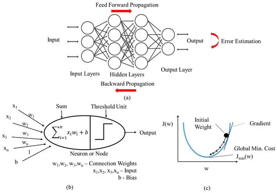 Figure 3. Structure of an artificial neural network (ANN) (a) ANN (b) single neuron or node (c) optimizing weights using gradient descent.
Table 5.
Exemplar classifier learning algorithm for classification of machine operating sounds.
Table 5.
Exemplar classifier learning algorithm for classification of machine operating sounds.
| SN | Classifier Learning Algorithms | Features | Application | Ref. |
|---|---|---|---|---|
| 1 | SVM | Frequency domain signal analysis: Band-power ratio | Detection of air leaks between grate bars lined sinter strand pallets in a sintering plant | [36] |
| 2 | Decision Tree (J48/C4.5 Algorithm) | Frequency domain signal analysis: Band-power ratio | Detection of air leaks between grate bars lined sinter strand pallets in a sintering plant | [36] |
| 3 | Deep Neural Network (DNN) | Frequency domain signal analysis: Short-Term Fourier Transform (STFT) | Detecting changes in electric motor operational states such as supply voltage and load | [14] |
| 4 | Decision tree, Naive Bayes, kNN, SVM, Discriminant Analysis, Ensemble classifier, with Bayesian Optimisation | Frequency domain signal analysis: Wavelet packet transform, with Principal Component Analysis (PCA) | Detecting of internal combustion engine fault | [40] |
| 5 | kNN, SVM, and Multi-layer Perceptron (MLP) | Frequency domain signal analysis: Wavelet packet transform with various mother wavelets | Detecting of internal combustion engine fault | [44] |
| 6 | Artificial Neural Network (ANN) | Frequency domain signal analysis: Spectral peaks from the fast Fourier Transform of acoustic signal (0–2996.25 Hz) | Detecting loose stator coils in induction electric motors | [6] |
2.2.2. Acoustic Image-Based Deep Learning Methods
This approach leverages techniques from the field of machine hearing [45]. Machine hearing involves sound processing considering inherent sound sensing system structures as humans and sound mixtures in realistic context [45].
In emulating human hearing, machine hearing adopts a four-layer architecture within which each layer represents a distinct area of research. The first layer, auditory periphery layer (cochlea model), mimics the representation of the nonlinear sound wave propagation mechanism in the cochlea as cascading filter systems; the second layer, auditory image computation, provides a projection of one or more forms of auditory images to the auditory cortex mimicking the auditory brain stem operation; the third layer abstracts the operation within the auditory cortex via extraction of application-dependent features from the auditory images; the final and forth layer addresses the application specific problem using appropriate machine learning system [46].
For application in classifying anomalous machine operating sound, variations are made in the auditory image computation representation; as such, best referred to as acoustic image representation. From the literature, there have been several possibilities for the 2D acoustic image representation such as: spectrogram (from STFT), Mel-spectrogram, cochleagram, amongst others [47,48]. Table 6 provides a summary of acoustic image representation in combination with deep learning models for classifying anomalous machine operating sounds and Figure 4 shows examples of acoustic image representations.
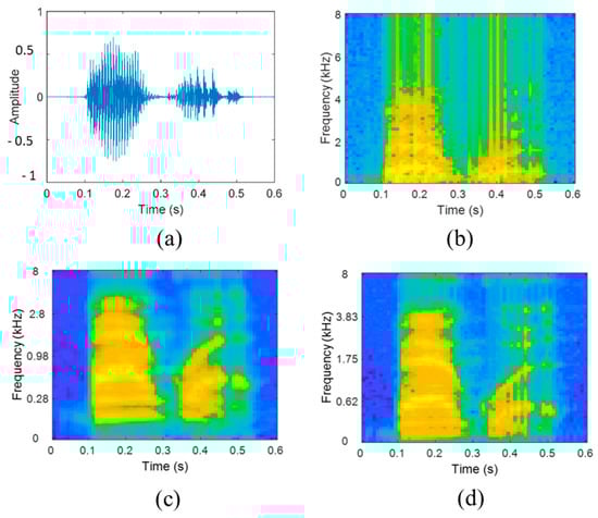
Figure 4.
Acoustic image representation (a) acoustic input (b) spectrogram of acoustic input (c) cochleagram of acoustic input (d) Mel spectrogram of acoustic input [16].
- (1)
- Acoustic Image Representation
- (a)
- Spectrogram: This is a two-dimensional representation of the frequency characteristics of a time-domain signal as it changes over time as shown in Figure 4. Spectrogram is generated using Fourier transform of the time-domain signal; the time-domain signal is first divided into smaller segments of equal length with some overlap; then, fast Fourier transform (FFT) is applied to each segment to determine its frequency spectrum; the resulting spectrogram becomes a side-by-side overlay of the frequency spectrum of each segment over time. FFT represents an algorithm to compute the discrete Fourier transform (DFT) of the windowed time-domain signal, represented as [16]:where is discrete Fourier transform, N is number of sample points within the window, is the discrete time-domain signal, and is the window function.The spectrogram is obtained as the logarithm of the DFT, as such [16]:where is spectrogram, and is discrete Fourier transform.
- (b)
- Mel Spectrogram: This is a spectrogram where frequencies have been transformed to the Mel scale as shown in Figure 5. The Mel scale is a linear scale model of the human auditory system, represented as [49,50]:where is frequency on the Mel scale, and f is frequency from the spectrum.
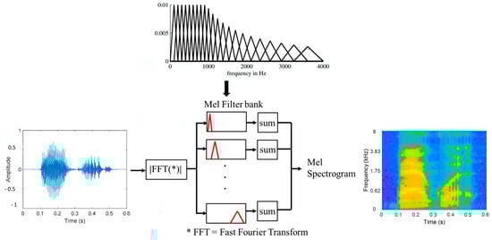 Figure 5. Mel spectrogram operation.
As shown in Figure 5, Mel spectrogram is computed by passing the result of windowed times-series signal FFT for each smaller segment of the divided signal through a set of half-overlapped triangular band-pass filter bank equally spaced on the Mel scale. The spectral values outputted from the Mel band-pass filter bank are summed and concatenated into a vector of size dependent on the number of Mel filters, e.g., 128, 512, etc. The resulting Mel spectrogram becomes a side-by-side overlay of the resulting vector representation from each consecutive time-series signal segment over time.
- (c)
- Cochleagram: A cochleagram is a time-frequency representation of the frequency filtering response of the cochlea (in the inner ear) as simulated by a bank of Gammatone filters [48]. The Gammatone filter represents a pure sinusoidal tone that is modulated by a Gamma distribution function; the impulse response of the Gammatone filter is expressed as [16]:where A is amplitude, n is filter order, b is filter bandwidth, is filter centre frequency, is phase shift between filters, and t is time.
As shown in Figure 6, cochleagram is computed by passing the result of windowed times-series signal FFT for each smaller segment of the divided signal through a series of overlapping band-pass Gammatone filter bank. The spectral values outputted from the Gammatone filter bank are further transformed by logarithmic and discrete cosine transform operations before been summed and concatenated into a vector of size dependent on the number of Gammatone filters, e.g., 128, etc. The resulting cochleagram becomes a side-by-side overlay of the resulting vector representation from each consecutive time-series signal segment over time.
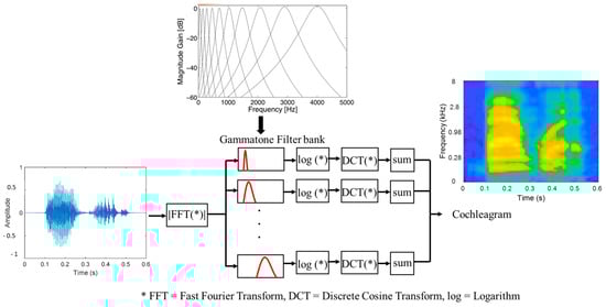
Figure 6.
Cochleagram operation.
- (2)
- Deep Learning Methods
- (a)
- Convolution Neural Network (CNN): CNN is inspired from the operation of the mammalian visual cortex. As shown in Figure 7, CNN is a multi-stage neural network made up of key stages: filter stage (i.e., convolution layer, pooling layer, normalisation layer and activation layer) and classification stage (i.e., fully connected layer of multilayer perceptron) [51]. The convolution layer functions to extract feature set from acoustic image representation into a feature map, pooling layer reduces the dimensionality of the feature map, and the classification stage performs the classification task using the multilayer perceptron. [47] has applied CNN with a combination of log-spectrogram, short-time Fourier transform and log-Mel spectrogram features to classify rolling-element bearing cage fault based on acoustics signals. Implemented CNN model consisted of three stage feature extraction layers: fully connected layer (shape = 16 × 16, rectified linear unit (ReLU) activation function, max. pooling = 2 × 2), fully connected layer (shape = 32 × 32, ReLU, max. pooling = 2 × 2), and fully connected layer (shape = 64 × 64, ReLU, max. pooling = 2 × 2) and a final classification stage based on multi-layer perception with 512 hidden nodes, ReLU and sigmoid activation function. Dataset was very sparse, and model was not optimized; therefore, impacting model performance on training accuracy. Table 6 highlights other applications of acoustic image-based classifiers of anomalous machine operating sounds.
 Figure 7. CNN basic architecture [51].
 - (b)
- Recurrent Neural Network (RNN): RNN is a type of neural network which uses sequential data or time series data to learn. Unlike CNN, RNN have internal memory state (i.e., can be trained to hold knowledge about the past); this is possible as inputs and outputs are not independent of each other, prior inputs influence the current input and output; simply put, output from previous layer state are feed back to the input of the next layer state. As shown in Figure 8, x is input layer, h is middle layer (i.e., consist of multiple hidden layers) and y is output layer. W, V and U are the parameters of the network such as weights and biases. At any given time (t), the current input is constituted from the input x(t) and previous x(t − 1); as such the output from x(t − 1) is feedback into the input x(t) to improve the network output. This way, information cycles through a loop within the hidden layers in the middle layer. RNN uses the same network parameters for every hidden layer, such as: activation function, weights, and biases (W, V, U). Despite the flexibility of the basic RNN model to learning sequential data, they suffer from the vanishing gradient problem (i.e., difficulty training the model when the weights get too small, and the model stops learning) and exploding gradient problem (i.e., difficulty training the model due to very high weight assignment). To overcome these challenges, the long short-term memory (LSTM) network variant of RNN is normally used. LSTM has the capability to learn long-term dependencies between time steps of sequential data. LSTM can read, write and delete information from its memory. It achieves this via a gating process made up of three stages: forget gate, update/input gate and output gate which interacts with is long-term memory and short-term memory pathways used to feedback its memory states amongst hidden layers. As shown in Figure 9, “c” represents the cell state and long-term memory, “h” represents the hidden state and short-term memory, and “x” represent the sequential data input. The forget gate determines how much of the cell state “c” is thrown away or forgotten. The update gate determines how much of new information is going to be stored in the cell state, and output gate determines what is going to be outputted. [52] has applied LSTM RNN with cochleagram features to classify varying rolling-element bearing faults based on 60 s acoustics signals. Implemented model consisted of an input feature set based on 128 gammatone filter bank cochleagram; Considering a 1 s. duration as a frame, the 60 s dataset generated 60-time frames. Each frame is represented as a cochleagram. 67% of the dataset was used to train the LSTM RNN model and 33% for testing. Model accuracy on fault classification task was 94.7%. Table 6 highlights other applications of acoustic image-based classifiers of anomalous machine operating sounds.
 Figure 8. RNN basic architecture.
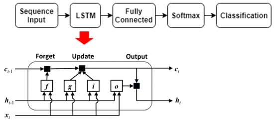 Figure 9. LSTM RNN architecture [52].
 - (c)
- Spiking Neural Network (SNN): SNN is a brain-inspired neural network where information is represented as binary events (spikes). It shares similarity with concepts such as event potentials in the brain. SNN incorporates time into its propagation model for information; SNN only transmit information when neuronal potential exceeds a threshold value. Working only with discrete timed events, SNS accepts as input spike train and outputs spike train. As such, information is required to be encoded into the spikes which is achieved via different encoding means: binary coding (i.e., all-or-nothing encoding with neurons active or inactive per time, rate coding, fully temporal codes (i.e., precise timing of spikes), latency coding, amongst others [53]. As shown in Figure 10, SNN is trained with the margin maximization technique, described in [54]. During first epoch, SNN hidden layer is developed based on neuron addition scheme. In subsequent epochs, the weights and biases of the hidden layer neurons are updated further using the margin maximization technique. Here, weights of the winner neuron are strengthened, while those of the others are inhibited; this reflects the Hebbian learning rule of the natural neurons; as a result, neurons are only connected to their local neurons, so they process the relevant input patterns together. This approach maximizes the margin among the classes which lends itself to training the spike patterns. Ref. [48] has applied SNN with cochleagram features to classify varying rolling-element bearing faults based on 10 s acoustics signals. Implemented model consisted of an input feature set based on 128 gammatone filter bank cochleagram; later reduced to 50 using principal component analysis (PCA). Considering a 10 ms duration as a frame, the 10 s dataset generated 1000-time frames. Each frame was encoded into a spike train using the population coding method. 90% of the dataset was used to train the SNN model and 10% for testing. Model accuracy was above 85%. Table 6 highlights other applications of acoustic image-based classifiers of anomalous machine operating sounds.
 Figure 10. SNN architecture [48].
Table 6.
Exemplar acoustic image representation and classifier models.
Table 6.
Exemplar acoustic image representation and classifier models.
| SN | Acoustic Image Representation | Deep Learning Methods | Application | Ref. |
|---|---|---|---|---|
| 1 | Spectrogram/Log-Spectrogram | CNN * | Detection of rolling-element bearing fault such as cage defect | [47] |
| RNN * | Detection of air leaks between grate bars lined sinter strand pallets in a sintering plant | [36] | ||
| 2 | Cochleagram | RNN * | Detection of rolling-element bearing fault such as inner race defect, outer race defect, rolling-element defect, combined defect, and heavily worn bearing | [52] |
| 3 | Cochleagram | SNN * | Detection of rolling-element bearing fault such as inner race defect, outer race defect, rolling-element defect, combined defect, and heavily worn bearing | [48] |
| 4 | Spectrogram (from STFT) | CNN * | Detection of rolling-element bearing fault such as cage defect | [47] |
| 5 | Log-Mel Spectrogram | CNN * | Detection of rolling-element bearing cage fault | [47,55] |
* CNN: Convolutional Neural Network, RNN: Recurrent Neural Network, SNN: Spiking Neural Network.
3. Datasets for Detection and Classification of Anomalous Machine Sound (DCAMS)
Openly available datasets are vital for progress in the data-driven machine condition monitoring approaches. In recent time, there have been significant progress in the corollary area of acoustic scene classification mainly due to opensource dataset such as: AudioSet dataset [1], which provides a collection over 2 million manually labelled 10 s sound segments from YouTube within 632 audio event classes. However, nothing of such large scale is available for Detection and Classification of Anomalous Machine Sounds (DCAMS). Within limited scale, several research projects are beginning to lay the foundation as they were bridging the dataset gap for DCAMS.
3.1. ToyADMOS Dataset
This dataset provided by [9], is a collection of anomalous machine sounds produced by miniaturised machines (i.e., toy car, toy conveyor, and toy train) as shown in Figure 11. It is designed to provide scenarios such as: inspecting machine condition (toy car), fault diagnostics for a static machine (toy conveyor) and fault diagnostics for a dynamic machine (toy train). The data acquisition setup for each scenario is performed using four microphones sampled at 48 kHz and measurement locations are shown in Figure 12. To provide anomalous operating conditions for the miniaturised machines, systematic fault modes as shown in Table 7 are imbedded in the various toy machines.
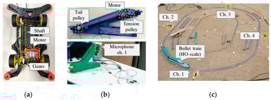
Figure 11.
Schematic of ToyADMOS miniaturised machines (a) toy car (b) toy conveyor (c) toy train [9].

Figure 12.
Schematic of microphone installation setup for ToyADMOS miniaturised machines (a) toy car (b) toy conveyor (c) toy train [9].
Table 7.
Imbedded faults in ToyADMOS miniaturized machines [9].
3.2. MIMII Dataset
The MIMII (Malfunctioning Industrial Machine Investigation and Inspection) dataset comprises normal and anomalous machine operating sounds of four types of real machines such as valves, pumps, fans, and slide rails [10]. The dataset was captured using an 8-microphone circular array with machine configuration in Figure 13 and sampled at 16 kHz. Each recording consists of 10 s. segments recordings of the machines with various faults as shown in Table 8.

Figure 13.
Schematic of microphone installation setup for MIMII [10].
Table 8.
Imbedded faults in MIMII real machines [10].
3.3. DCASE Dataset
The DCASE dataset [13] is a merge of subset of ToyADMOS and MIMII dataset comprising both normal and anomalous machine operating sounds. To harmonise both datasets, each audio file includes a single channel and 10 s in duration. All the audio files are resampled at 16 kHz. The dataset relates to the following machine operating sounds: toy car (ToyADMOS), toy conveyor (ToyADMOS), valve (MIMII), pump (MIMII), fan (MIMII) and slide rail (MIMII).
3.4. IDMT-ISA-ELECTRIC-ENGINE Dataset
The IDMT-ISA-ELECTRIC-ENGINE dataset [14] consists of anomalous operating sounds of three brushless electric motors. Different operational states such as good, heavy load and broken are simulated within the electric motors by changing the supply voltage and loads. The dataset provides mono audio for each sound file sampled at 44.1 kHz. For each of the operational states, IDMT-ISA-ELECTRIC-ENGINE dataset provides 774 sound files for “good” state, 789 for “broken” state and 815 for “heavy load”. Figure 14 shows the setup for acoustic data acquisition in the electric motor machines.
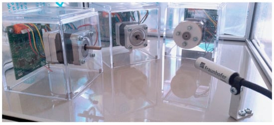
Figure 14.
Three electric motor setups for IDMT-ISA-ELECTRIC-ENGINE dataset [14].
3.5. MIMII DUE Dataset
The MIMII DUE (Malfunctioning Industrial Machine Investigation and Inspection with domain shifts due to changes in operational and environmental conditions) provides a sound dataset for training and testing anomalous sound detection techniques and their invariance to domain shifts [56]. This builds on the authors’ previous released MIMII dataset [10] which had the limitation of not representing industrial scenarios with changes in machine operational speed and background noises.
MIMII DUE provides normal and anomalous sounds for five industrial machines: fan, gearbox, pump, slide rail and valve. For each of the machines, six sub-division is provided referred to as sections. Each section refers to a unique instance of machine product; this provides for manufacturing variability within machine type. Furthermore, each section has its dataset is split into source domain and target domain. The source domain contains machine operating sound running at design point while target domain contains machine operating sound running at off-design point.
3.6. ToyADMOS2 Dataset
ToyADMOS2 dataset also provides for training and testing anomalous machine sound detection techniques for their performance in domain shifted conditions [57]. As opposed to ToyADMOS its predecessor, it only carters for two types of miniature machines: toy car and toy trains. The recording and system setup is same for ToyADMOS [9]; however, a key difference, ToyADMOS2 has the normal and anomalous machine operating sounds recorded with machines operating under different speeds. This provides for a source domain consisting of machines with specified operating conditions and the target domain with machines having different operating conditions. Suitable for training and testing with the different domains.
3.7. MIMII DG Dataset
MIMII DG dataset provides normal and anomalous machine operating sounds for benchmark Domain Generalisation techniques [58]. It comprises five groups of machines including valve, gearbox, fan, slide rail and bearing. The audio recording for each machine consists of three sections representing different types of domain shift conditions, which for each machine could be operating condition change and environmental background noise change.
4. Challenges
4.1. Sound Mixtures with Background Noise
The presence of background noise interfering with machine fault signature during acquisition of acoustic data poses a challenge in terms of accuracy and repeatability of machine fault diagnostics. Background noise in this context refers to sound from other operating machines that are different from the target machine. Additionally, it includes the sounds from other activities in the industrial environment.
Approaches are therefore required to eliminate background noise from the collected acoustic data. The challenge lies in the fact that the background noise sources are uncorrelated, as such, filtering techniques are not applicable. Techniques, such as Blind Signal Separation (BSS) and Independent Component Analysis (ICA), have the potential to address this challenge by recovering the signal of interest out of the observed sound mixtures. BSS has been applied in [59] for extracting the unobserved fault acoustic signal during metal stamping with a mechanical press. Wang et al. [60] also applied BSS using sparse component analysis for separating sound mixtures of power transformer origin. In [48], ICA was applied together with variational mode decomposition, to separate the independent components hidden in the observation low signal-to-noise ratio signals, for an intelligent diagnosis application.
In practice, the mixture of acoustic signals is formed by the random mixing of multiple sound sources resulting in non-linear mixture models, which is an area requiring further attention for acoustic-based machine condition monitoring.
4.2. Domain Shift with Changes in Machine Operation and Background Noise
Domain shift represents the change in machine operating and environmental conditions. This is common in industrial settings as machines would not always operate in their design point conditions. There is always a need for the machine to run at an off-design point, indicating changes to both speed and loading as well as changes in the background noise from auxiliaries during operation. Tackling the domain shift problem is important for effective anomaly detectors applicable to machine operating sound.
The concept of domain adaptation is gaining prominence as an approach for anomaly detection in domain shifted conditions [11,61]. Domain adaptation addresses the problem as: when provided with a set of normal data from a source domain and a limited set of normal data from a target domain, how do you develop a performant anomaly detector in the target domain. From the literature, the following approaches for domain adaptation have emerged: learning the transformation from the source domain to the target domain [62,63], learning invariant representations between the source and the target domains [64,65,66,67] and few-shot domain adaptation [68,69]. With the option of domain adaptation, it opens opportunities for application to acoustic-based machine condition monitoring and fault diagnostics.
4.3. Domain Generalisation Invariant to Changes in Machine Operation and Background Noise
Domain generalisation is an attempt to provide an alternative to the domain adaptation techniques when dealing with domain shift due to the computational cost of the domain adaptation techniques. Domain generalisation poses the problem of learning commonalities across various domains (i.e., source and target) to enable the model to generalize across the domains. Such generalisation would need to account for domain shift caused by differences in environmental conditions, machine physical conditions, changes due to maintenance, and differences in recording devices for instance.
Fundamentally, domain generalisation attempts the out-of-distribution generalisation by using only the source domain data. In the literature, several techniques have emerged such as [70]: domain alignment, meta-learning, ensemble learning, data augmentation, self-supervised learning, learning disentangled representations, regularisation strategies, and reinforcement learning. With the development and application of domain generalisation techniques for machine fault diagnostics problem, it would open compelling opportunities for the applicability of the acoustic-based approaches.
4.4. Effect of Measurement Distance, Measurement Device and Sampling Parameters
4.4.1. Measurement Distance (Microphones Positions)
Sound propagates through air as a longitudinal wave; as it moves through the air medium, from the source to the listener or observer, sound as characterised by sound intensity, experiences attenuation, i.e., loss in energy. For a point source (i.e., uniformly radiating sound in all directions), this attenuation follows the inverse square law as shown in Figure 15, which is dependent on the measurement distance. In practice, for every doubling of measurement distance, the sound intensity reduces by a factor of 4; alternatively, the sound pressure level reduces by 6 dB. From sound propagation theory, it is evident that, the measurement distance of anomalous machine operating sound is important [71]. However, very little consideration has been given to this effect during experimental setup for anomalous machine sound data acquisition as corroborated by the benchmarking opensource datasets such as ToyADMOS, MIMII, IDMT-ISA-ELECTRIC ENGINE, MIMII DUE, ToyADMOS2, and MIMII DG. One can argue, the measurement distance effect can be accounted for within domain adaptation or domain generalisation challenges. Yet, the various datasets do not provide a systematic grouping of the dataset based on the measurement distance for this to be considered. The parameters often considered are changes in machine operating parameters (i.e., rotating speed and load) and environmental/background noise.
An important question is then raised; how far should the microphones be from the sound source considering the measurement distance effect?
In acoustics, two physical regions exist that shed light to the above question: the acoustics near field and acoustics far field as shown in Figure 16. The transition from near field to far field occur in at least 1 wavelength of the sound source [72]. It is important, to note, as wavelength is a function of frequency, this transition distance would change as the frequency content of the sound source changes. The near field exist very close to the sound source with no fixed relationship between sound intensity and distance. Within the far field, the inverse square law of sound propagation holds true. In practice, this is the region where the measuring microphone should ideally be located. As a minimum, a single microphone can suffice for accurate and repeatable measurement of sound. Although fundamental acoustics theory would place the far field at least 1 wavelength of the sound source [72]; ISO 3745, provides several guidelines or criteria for microphone placement within the far field for sound power measurement [73]:
where r is measurement distance, is characteristic dimension or largest dimension of the sound source, and is the lowest wavelength of the sound source.
For small, low-noise sound sources with measurement over a limited frequency range, the measurement distance can be less than 1 m, but not less than 0.5 m, provided consideration for criteria (a) and (b) above are adhered to [73].
Within the near field, measurement is feasible; but would require multi-microphone array. For the measurement of anomalous machine operating sound, guidelines are lacking in the literature and further research is required.

Figure 15.
Distance effect on sound intensity propagation and attenuation [74].
Figure 15.
Distance effect on sound intensity propagation and attenuation [74].


Figure 16.
Acoustic sound field consideration [72].
Figure 16.
Acoustic sound field consideration [72].

4.4.2. Single Microphone Measurement Device and Sampling Parameters
Acoustic measuring device mismatch between development data acquisition and testing can occur in practice. As every microphone have its unique transfer function which dictates its frequency response and perception of sound, measuring device mismatch needs to be considered. Very little has been done in considering this challenge in the detection and classification of anomalous machine operating sound. However, such consideration is already attracting attention in the corollary field of acoustic scene classification [75]. Key to this consideration in acoustic scene classification field, is the realization of the TUT Urban Acoustic Scenes dataset which consists of ten different acoustic scenes, recorded in six large European cities with four different microphone devices: highlighting the importance of considering the acoustic measuring device for robust pattern learning algorithm [75].
As very little work has been explored on the effect of recording device mismatch in anomalous machine operating sound detection and classification to inform device choice; still, some learning can be gleaned from the choice of microphones, sampling frequency and sample duration as shown in Table 9 from the opensource dataset projects on DCAMS.
Table 9.
Exemplar acoustic measurement devices and sampling parameters.
4.4.3. Microphone Array Measurement (Acoustic Camera)
Acoustic camera measurement provides the capability for sound source localisation, quantification and visualization using multi-dimensional acoustic signals processed from a microphone array unit and overlaid on either image or video of the sound source as shown in Figure 17 [76]. An acoustic camera, is a collection of several microphones, acting as a microphone array unit, where the microphones within the array can be arranged either as uniform circular configuration, uniform linear configuration, uniform square configuration or customized array configuration for specific application. Acoustic camera can provide acoustic scene measurement both in the near and far acoustic fields.
For localizing anomalous machine operating sound in application, acoustic camera has been used to map the variation in machine emitted sound for fault detection as follows: localizing sources of aircraft fly by noise [77], characterising emitted sound from internal combustion engine running idle in a vehicle [78], fault detection in a gearbox unit [79], fault localisation in rolling-element bearing [80], etc.

Figure 17.
Acoustic camera for fault detection based on variation in emitted sound (a) Acoustic camera setup (b) test object without a fault (c) test object with a fault [81].
Figure 17.
Acoustic camera for fault detection based on variation in emitted sound (a) Acoustic camera setup (b) test object without a fault (c) test object with a fault [81].

Central to the analysis and interpretation of the multi-dimensional acoustic signals is acoustic beamforming technique [76,82]. Ref. [82] provides an extensive review on acoustic beamforming theory including consideration for acoustic beamforming test design criteria.
Acoustic beamforming is a spatial filtering technique used in far field acoustic domain, for localisation and quantification of the sound source; where it amplifies the acoustic signal of interest while suppressing interfering sound sources (e.g., background noise) [82]. In principle, the beamforming algorithm works by summing individual acoustic signals based on their arrival times from the sound source to the microphone array. This summation process suppresses the interfering signals while enhancing the acoustic signal of interest. The technique can be performed both in the time-domain and frequency domain [82].
- (1)
- Delay and Sum Beamforming in the Time-Domain: This is demonstrated in Figure 18 as follows, considering only two sound sources as an example (i.e., source 1 and source 2). For each sound source, the travel path of emitted sound to the microphone array would be different; as such, captured signals by the microphone array would show different delays and phases for the measured signals from both sources. As both parameters, delay, and phase, are proportional to the travelled distance between microphone array and source; with the knowledge of the speed of sound in the medium (e.g., air), the runtime delay is estimated for the signal of interest (source 1) reaching all the microphone locations. The measured signal for every microphone in the array is then shifted by the calculated runtime delay for that channel, creating an alignment in phase in the time-domain for the signal of interest (source 1). The resulting signals from every microphone channel are summed and normalised by the number of microphones in the array; As shown in Figure 18, the signal of interest (source 1) is amplified due to constructive interference while source 2 is minimized due to destructive interference. To create the final acoustic scene representation, for each microphone channel, the root mean square (RMS) amplitude value or the maximum amplitude value of the time-domain acoustic signal can be evaluated for visualization as an acoustic map.
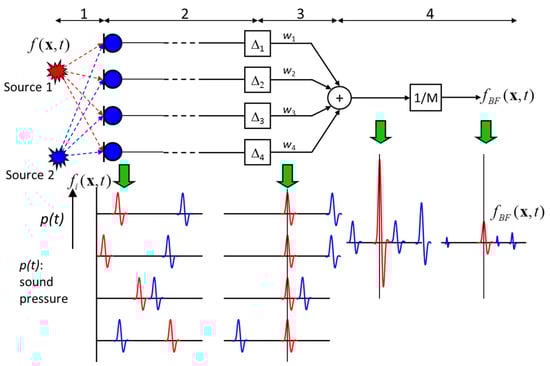 Figure 18. Schematic of delay and sum beamforming in the time domain for acoustic sources [83].
 - (2)
- Delay and Sum Beamforming in the Frequency Domain: This is demonstrated in Figure 19 as follows, considering only two sound sources as an example (i.e., source 1 and source 2). For each sound source, the travel path of emitted sound to the microphone array would be different; as such, captured signals by the microphone array would show different delays and phases for the measured signals from both sources. The delay for the signal of interest can be determined using information such as, distance between source and microphone and the speed of sound in the medium. Fourier transform is performed at all microphone channel resulting in a complex spectrum for amplitude and phase. To eliminate the delay in phase for the signal of interest at all microphone location, the complex spectra is multiplied by a complex phase term as shown in Figure 19, bringing the interested acoustic source in phase without impacting the amplitude of the spectra. The resulting complex spectra from all the microphone channels are summed and normalised by the number of microphone channels. The interest sound source signal (source 1) is enhanced due to constructive interference, while source 2 is diminished due to destructive interference.
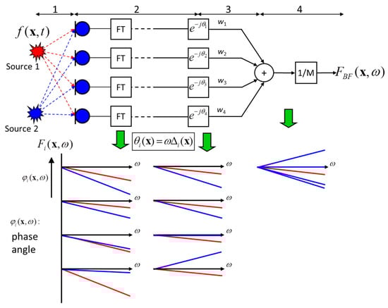 Figure 19. Schematic of delay and sum beamforming in the frequency domain for acoustic sources [84].
Application of acoustic camera to machine diagnostics have been attracting increasing interest [77,78,79,80,85,86]. Of note, is the approach proposed by [85,86] to localise faults in rotating machinery using acoustic beamforming and spectral kurtosis (i.e., spectral kurtosis is an effective indicator of machine fault [87,88]). As shown in Figure 20, spectral kurtosis is used as a post-processor of the multi-dimensional acoustic time-domain signals from the microphone array to identify and localise fault-related frequency bands (i.e., frequency bands that are impulsive); the resulting kurtogram having a spatial dimension provides the capability to localise the high kurtosis region providing indication of machine fault.
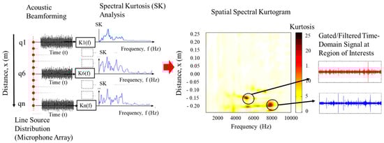
Figure 20.
Application of spectral kurtosis to acoustic beamforming for machine fault diagnosis [85,86].
5. Outlook
Anomalous machine operating sound provides a rich set of information about a machine’s current health state upon which to automate the detection and classification of machinery faults. Despite advances in data-driven machine learning and deep learning approaches as currently applied for acoustic-based machine condition monitoring, there still exist areas for further research for this technique to be industrially applicable.
5.1. Addressing Pitfalls in Acoustic Data Collection
The performance of data-driven models and their ability to generalize during training and testing depends on the available datasets being a representative of the actual fault scenario. However, generating machine fault dataset for actual machines is a costly endeavor. If the training dataset is too small, the model learns sampling noise. As a work around, most of the opensource dataset for the detection and classification of anomalous machine operating sounds have focused on either toy machines or scaled down machine models. This approach has provided initial seeding to be able to benchmark currently developed techniques. Generally, available datasets account for steady-state changes in machine operational parameters such as speed and load, consideration of varying degree of background noise during acoustic signal measurement, and different models of similar machine class. These datasets are lacking in the following areas: consideration of the distance effect during grouping of the dataset (i.e., it would be relevant to have measurements at different distances from the source to test the robustness of developed approaches working in the field where it would be difficult to maintain repeatable measurement distance), consideration of transient operation regime of machines during dataset grouping (i.e., steady-state dataset alone is a non-representative training data; developed approach need to be able to differentiate transient operation from anomalous operation), and consideration of device mismatch during data acquisition (i.e., recording for same machine fault with different types of microphones, such as omni-directional microphone, pressure-free field microphone, condenser microphone, etc.; Furthermore, it would be relevant to specify a standard reference microphone such as the omni-directional microphone, in other for spectrum correction coefficients for various microphones to be provided with respect to this [89]; using spectrum correction coefficients opens up the possibility of data transformation to account for device mismatch).
5.2. Addressing Measurement Artifacts (i.e., Background Noise, and Distance Effect)
In the industrial environment, acoustic-based machine condition monitoring is often plagued with the problem of having multiple signals mixing such as acoustic signal of interest indicative of anomalous machine operation and the background noise, i.e., neighboring machinery, factory noise, etc. It is required for the sound mixture to be separable, i.e., separating the acoustic signal of interest from the background noise. Conventional approaches such as spectral subtraction methods which rely on the background noise having a constant magnitude spectrum and acoustic signal of interest been short-time stationary would not be applicable as there is the possibility of removing fault frequencies from the spectrum of the acoustic signal of interest [90]. Blind signal separation can be useful as it offers sound mixture separation without prior knowledge of either of the signals or the way in which they are mixed [91]. Application and optimisation of blind signal separation for acoustic-based machine condition monitoring provides an area for further research.
The effect of distance between the acoustic source and microphone leads to attenuation of the measured sound intensity. Furthermore, it places a burden of repeatability between laboratory conditions and industrial conditions, impacting data-driven model accuracy for application. Eliminating or minimizing the distance effect on the acquired acoustic signal is an area requiring further research. [71] proposed a normalisation scheme (i.e., d-normalization) in the frequency domain using the spectrum representation of the acoustic signal which minimized the distance effect as shown in Figure 21 and expressed as:
where is the normalised spectrum of the measured sound intensity, is the un-normalised spectrum of the measured sound intensity (i.e., determined from fast Fourier transform of the time-domain acoustic signal), and is the mean of the rectified time-domain acoustic signal intensity, given as:
where N is number of sample points in the acoustic time-domain signal, is the absolute amplitude value of the acoustic time-domain signal.
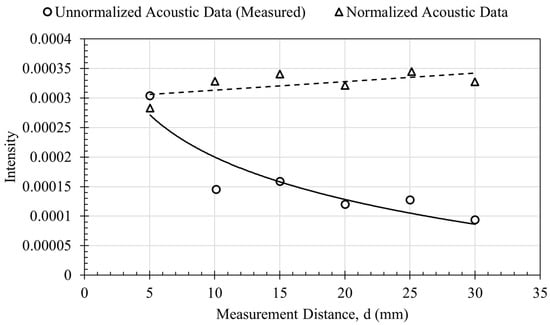
Figure 21.
Minimizing distance effect on measured acoustic signal using d-normalisation [71].
Although the result is promising, it is applicable to the spectral representation of the acoustic signal. Alternative normalisation scheme be required for other acoustic image representation such as cochleagram, Mel-spectrogram, amongst others? Furthermore, what would be the impact on the data-driven model accuracy due to normalisation of the input acoustic representation? These are open questions for further research.
5.3. Improving Data-Driven Model Accuracy for Application: Domain Adaptation versus Domain Generalisation
Domain shift (i.e., changes in machinery operating speed and load) is inevitable in industrial processes due to machines operating in off-design conditions and harsh environment. As such, training data-driven models for the DCAMS problem to account for this system dynamics is a must have. However, learning robust model representation by using data from multiple domains to identify invariant relationships between the various domains is still a challenging problem. Two schools of thought have emerged to address the domain shift problem in acoustic-based machine condition monitoring: domain adaptation [92,93] and domain generalisation [94]. Both approaches tackle the same problem based on the available dataset. Domain adaptation assumes you have dataset from the source domain (i.e., machine operating at design point) and some set of data in the target domain (i.e., machine operating at off-design point), it attempts to learn the mapping between the source and target domain based on these criteria. Alternatively, domain generalisation assumes you have dataset from two different source domains, it attempts to learn the mapping to an unseen domain. Although several domain adaptation and generalization techniques have been proposed in the literature, the model performance for both approaches is yet to reach satisfactory level in applications as evident from DCASE2021 and DCASE2022 Task 2 challenges [11,12].
5.4. Addressing Multi-Fault Diagnosis
In industrial environment, machinery may need to operate in both off-design conditions and harsh conditions continuously for extended periods of time. As such, machine components are liable to the occurrence of multiple faults at the same time. When these multi-faults occur, their impact to machine performance and lifespan is more severe as compared to the presence of a single fault due to fault interactions [95]. Fault diagnosis approaches needs to be able to accommodate both single fault and multi-faults detection scenarios. From the literature, within acoustic-based condition monitoring methodology, the focus has been on addressing the single-fault diagnosis problem; multi-fault diagnosis of machinery is still lacking. This area of research needs consideration for viable industrial applications, e.g., fault diagnosis in gearbox, electric motor, compressor, pump, amongst others.
5.5. Improving Acoustic Camera Spatial Detection of Machine Faults
Acoustic camera for machine fault diagnosis provides spatial information not possible with conventional condition monitoring approaches such vibration analysis. However, interpreting the visualization of the emitted sound field from the machine from acoustic beamforming is very limited; It is important to note that regions of high sound pressure level does not necessarily correlate with the presence of a fault. Further research is required to analyse the multi-dimensional acoustic time-domain signals as a function of space from the acoustic beamforming analysis using either signal processing methods or data-driven machine learning/deep learning approaches. Pioneering in this regard, [85,86] have proposed spectral kurtosis as means to filter the multi-dimensional acoustic time-domain signals from acoustic beamforming to localise impulsive-related machine faults, e.g., gearbox faults, rolling-element bearing faults, etc., as well as extract the time-domain acoustic signals from the region of high spectral kurtosis. This area of research is still limited in correlating regions of high spectral kurtosis to a fault. The extract time-domain signal provides an opportunity to be explored for evaluation using data-driven approaches. Furthermore, beyond spectral kurtosis, what other signal processing approaches are relevant with improved sensitivity to localizing machine faults from the multi-domain acoustic signals provided by the acoustic camera?
6. Conclusions
Acoustic-based machine condition monitoring has been attracting increasing attention, especially with the annual DCASE challenge task on unsupervised anomalous sound detection for identifying machine conditions. Given the industrial relevance and significance of this research area, it becomes important in this paper to address the following questions: (i) are there commonalities or differences amongst the developed methodologies for detecting and classifying anomalous machine operating sounds, (ii) what open datasets are available for benchmarking the developed techniques, and (iii) what challenges are still there for the applicability of acoustic-based machine condition monitoring. Hopefully, this review of the state-of-the-arts can inspire more advancement in the acoustic-based machine condition monitoring research area.
Author Contributions
Conceptualization, G.J. and Y.Z.; writing—original draft preparation, G.J.; writing—review and editing, Y.Z. All authors have read and agreed to the published version of the manuscript.
Funding
This research received no external funding.
Data Availability Statement
Data sharing not applicable.
Conflicts of Interest
The authors declare no conflict of interest.
References
- Gemmeke, J.F.; Ellis, D.P.W.; Freedman, D.; Jansen, A.; Lawrence, W.; Moore, R.C.; Plakal, M.; Ritter, M. Audio Set: An Ontology and Human-Labeled Dataset for Audio Events. In Proceedings of the 2017 IEEE International Conference on Acoustics, Speech and Signal Processing (ICASSP), New Orleans, LA, USA, 5–9 March 2017; pp. 776–780. [Google Scholar]
- Cramer, J.; Wu, H.-H.; Salamon, J.; Bello, J.P. Look, Listen, and Learn More: Design Choices for Deep Audio Embeddings. In Proceedings of the IEEE International Conference on Acoustics, Speech and Signal Processing (ICASSP), Brighton, UK, 12–17 May 2019; pp. 3852–3856. [Google Scholar]
- Arandjelović, R.; Zisserman, A. Look, Listen and Learn. In Proceedings of the IEEE International Conference on Computer Vision (ICCV), Venice, Italy, 22–29 October 2017. [Google Scholar]
- Kong, Q.; Cao, Y.; Iqbal, T.; Wang, Y.; Wang, W.; Plumbley, M. PANNs: Large-Scale Pretrained Audio Neural Networks for Audio Pattern Recognition (Pretrained Models). IEEE/ACM Trans. Audio Speech Lang. Process. 2020, 28, 2880–2894. [Google Scholar] [CrossRef]
- Hershey, S.; Chaudhuri, S.; Ellis, D.P.W.; Gemmeke, J.F.; Jansen, A.; Moore, R.C.; Plakal, M.; Platt, D.; Saurous, R.A.; Seybold, B.; et al. CNN architectures for large-scale audio classification. In Proceedings of the 2017 IEEE International Conference on Acoustics, Speech and Signal Processing (ICASSP), New Orleans, LA, USA, 5–9 March 2017; pp. 131–135. [Google Scholar] [CrossRef]
- Gaylard, A.; Meyer, A.; Landy, C. Acoustic Evaluation of Faults in Electrical Machines. In Proceedings of the 1995 Seventh International Conference on Electrical Machines and Drives (Conf. Publ. No. 412), Durham, UK, 11–13 September 1995; pp. 147–150. [Google Scholar]
- Kawaguchi, Y.; Endo, T. How Can We Detect Anomalies from Subsampled Audio Signals? In Proceedings of the 2017 IEEE 27th International Workshop on Machine Learning for Signal Processing (MLSP), Tokyo, Japan, 25–28 September 2017; pp. 1–6. [Google Scholar]
- Koizumi, Y.; Saito, S.; Uematsu, H.; Harada, N. Optimizing Acoustic Feature Extractor for Anomalous Sound Detection Based on Neyman-Pearson Lemma. In Proceedings of the 2017 25th European Signal Processing Conference (EUSIPCO), Kos, Greece, 28 August–2 September 2017; pp. 698–702. [Google Scholar]
- Koizumi, Y.; Saito, S.; Uematsu, H.; Harada, N.; Imoto, K. ToyADMOS: A Dataset of Minia-ture-Machine Operating Sounds for Anomalous Sound Detection. In Proceedings of the 2019 IEEE Workshop on Applications of Signal Processing to Audio and Acoustics (WASPAA), New Paltz, NY, USA, 20–23 October 2019; pp. 313–317. [Google Scholar]
- Purohit, H.; Tanabe, R.; Ichige, T.; Endo, T.; Nikaido, Y.; Suefusa, K.; Kawaguchi, Y. MIMII Dataset: Sound Dataset for Malfunctioning Industrial Machine Investigation and Inspection. In Proceedings of the Detection and Classification of Acoustic Scenes and Events 2019 Workshop (DCASE2019), New York, NY, USA, 25–26 October 2019; pp. 209–213. [Google Scholar]
- Kawaguchi, Y.; Imoto, K.; Koizumi, Y.; Harada, N.; Niizumi, D.; Dohi, K.; Tanabe, R.; Purohit, H.; En-do, T. Description and Discussion on DCASE 2021 Challenge Task 2: Unsupervised Anomalous Sound Detection for Machine Condition Monitoring under Domain Shifted Conditions. arXiv 2021, arXiv:2106.04492. [Google Scholar]
- Dohi, K.; Imoto, K.; Harada, N.; Niizumi, D.; Koizumi, Y.; Nishida, T.; Purohit, H.; Endo, T.; Yamamoto, M.; Kawaguchi, Y. Description and Discussion on DCASE 2022 Challenge Task 2: Unsupervised Anomalous Sound Detection for Machine Condition Monitoring Applying Domain Generalization Tech-niques. arXiv 2022, arXiv:2206.05876. [Google Scholar]
- Koizumi, Y.; Kawaguchi, Y.; Imoto, K.; Nakamura, T.; Nikaido, Y.; Tanabe, R.; Purohit, H.; Suefusa, K.; Endo, T.; Yasuda, M.; et al. Description and Discussion on DCASE2020 Challenge Task2: Unsupervised Anomalous Sound Detection for Machine Condition Monitorin. In Proceedings of the Detection and Classification of Acoustic Scenes and Events 2020 Workshop (DCASE2020), Tokyo, Japan, 2–4 November 2020; pp. 81–85. [Google Scholar]
- Grollmisch, S.; Abeßer, J.; Liebetrau, J.; Lukashevich, H. Sounding Industry: Challenges and Datasets for Industrial Sound Analysis. In Proceedings of the 2019 27th European Signal Processing Conference (EUSIPCO), A Coruña, Spain, 2–6 September 2019; pp. 1–5. [Google Scholar]
- Koizumi, Y.; Saito, S.; Uematsu, H.; Kawachi, Y.; Harada, N. Unsupervised Detection of Anomalous Sound Based on Deep Learning and the Neyman–Pearson Lemma. IEEE/ACM Trans Audio Speech Lang Process 2019, 27, 212–224. [Google Scholar] [CrossRef]
- Sharan, R.; Xiong, H.; Berkovsky, S. Benchmarking Audio Signal Representation Techniques for Classification with Convolutional Neural Networks. Sensors 2021, 21, 3434. [Google Scholar] [CrossRef]
- Roche, F.; Hueber, T.; Limier, S.; Girin, L. Autoencoders for Music Sound Modeling: A Com-parison of Linear, Shallow, Deep, Recurrent and Variational Models. In Proceedings of the 16th Sound & Music Computing Conference (SMC 2019), Malaga, Spain, 28–31 May 2019. [Google Scholar]
- Bai, J.; Chen, C.; Chen, J. Feature Based Fusion System for Anomalous Sounds Monitoring. In Proceedings of the 5th Workshop on Detection and Classification of Acoustic Scenes and Events (DCASE), Tokyo, Japan, 2–4 November 2020. [Google Scholar]
- Ahmed, F.; Nguyen, P.; Courville, A. An Ensemble Approach for Detecting Machine Failure from Sound. In Proceedings of the 5th Workshop on Detection and Classification of Acoustic Scenes and Events (DCASE), Tokyo, Japan, 2–4 November 2020. [Google Scholar]
- Alam, J.; Boulianne, G.; Gupta, V.; Fathan, A. An Ensemble Approach to Unsupervised Anomalous Sound Detection. In Proceedings of the 5th Workshop on Detection and Classification of Acoustic Scenes and Events (DCASE), Tokyo, Japan, 2–4 November 2020. [Google Scholar]
- Morita, K.; Yano, T.; Tran, K.Q. Anomalous Sound Detection by Using Local Outlier Factor and Gaussian Mixture Model. In Proceedings of the 5th Workshop on Detection and Classification of Acoustic Scenes and Events (DCASE), Tokyo, Japan, 2–4 November 2020. [Google Scholar]
- Hendrycks, D.; Mazeika, M.; Dietterich, T. Deep Anomaly Detection with Outlier Exposure. In Proceedings of the Seventh International Conference on Learning Representations, Vancouver, BC, Canada, 30 April–3 May 2018. [Google Scholar]
- Sandler, M.; Howard, A.G.; Zhu, M.; Zhmoginov, A.; Chen, L.-C. Inverted Residuals and Lin-ear Bottlenecks: Mobile Networks for Classification, Detection and Segmentation. In Proceedings of the IEEE conference on computer vision and pattern recognition, Salt Lake City, UT, USA, 18–22 June 2018. [Google Scholar]
- Heng, R.B.W.; Nor, M.J.M. Statistical Analysis of Sound and Vibration Signals for Monitor-ing Rolling Element Bearing Condition. Appl. Acoust. 1998, 53, 211–226. [Google Scholar] [CrossRef]
- Van Riesen, D.; Schlensok, C.; Henrotte, F.; Hameyer, K. Acoustic Measurement for Detecting Manufacturing Faults in Electrical Machines. In Proceedings of the 17th International Conference on Electrical Machines (ICEM), Chania, Greece, 2–5 September 2006. [Google Scholar]
- Benko, U.; Petrovcic, J.; Juričić, Đ.; Tavčar, J.; Rejec, J. An Approach to Fault Diagnosis of Vac-uum Cleaner Motors Based on Sound Analysis. Mech. Syst. Signal Process. 2005, 19, 427–445. [Google Scholar] [CrossRef]
- Mishra, R.; Gu, F.; Fazenda, B.; Stubbs, C.; Ball, A. Measurement and Characterisation of Faults in the Intake System of a Turbocharged Engine Using a Directional Acoustic Probe. In Proceedings of the COMADEM 2009, San Sebastian, Spain, 9–11 June 2009. [Google Scholar]
- Wu, Z.; Huang, N.E. Ensemble Emprical Mode Decomposition: A Noise-Assisted Data Analysis Method. Adv. Adapt. Data Anal. 2009, 1, 1–41. [Google Scholar] [CrossRef]
- Fazenda, B.M. Acoustic Based Condition Monitoring of Turbine Blades. In Proceedings of the 18th International Congress on Sound and Vibration, Rio de Janeiro, Brazil, 10–14 July 2011. [Google Scholar]
- Grebenik, J.; Bingham, C.; Srivastava, S. Acoustic Diagnostics of Electrical Origin Fault Modes with Readily Available Consumer-Grade Sensors. IET Electr. Power Appl. 2019, 13, 1946–1953. [Google Scholar] [CrossRef]
- Shiri, H.; Wodecki, J.; Ziętek, B.; Zimroz, R. Inspection Robotic UGV Platform and the Proce-dure for an Acoustic Signal-Based Fault Detection in Belt Conveyor Idler. Energies 2021, 14, 7646. [Google Scholar] [CrossRef]
- Fang, S.; Li, S.-C.; Zhen, D.; Shi, Z.; Gu, F.; Ball, A.D. Acoustic Feature Extraction for Monitor-ing the Combustion Process of Diesel Engine Based on EMD and Wavelet Analysis. Int. J. COMADEM 2017, 20, 25–30. [Google Scholar]
- Zhen, D.; Wang, T.; Gu, F.; Tesfa, B.; Ball, A. Acoustic Measurements for the Combustion Di-agnosis of Diesel Engines Fuelled with Biodiesels. Meas. Sci. Technol. 2013, 24, 055005. [Google Scholar] [CrossRef][Green Version]
- Anami, B.S.; Pagi, V.B. Acoustic Signal-Based Approach for Fault Detection in Motorcycles Using Chaincode of the Pseudospectrum and Dynamic Time Warping Classifier. IET Intell. Transp. Syst. 2014, 8, 21–27. [Google Scholar] [CrossRef]
- Amarnath, M.; Sugumaran, V.; Kumar, H. Exploiting Sound Signals for Fault Diagnosis of Bearings Using Decision Tree. Measurement 2013, 46, 1250–1256. [Google Scholar] [CrossRef]
- Pasha, S.; Ritz, C.; Stirling, D.; Zulli, P.; Pinson, D.; Chew, S. A Deep Learning Approach to the Acoustic Condition Monitoring of a Sintering Plant. In Proceedings of the APSIPA Annual Summit and Conference 2018, Hawaii, HI, USA, 12–15 November 2018. [Google Scholar]
- Giannakopoulos, T. PyAudioAnalysis: An Open-Source Python Library for Audio Signal Analysis. PLoS ONE 2015, 10, e0144610. [Google Scholar] [CrossRef]
- Russell, S.J.; Norvig, P. Artificial Intelligence: A Modern Approach, 3rd ed.; Pearson: Boston, MA, USA, 2010. [Google Scholar]
- Raschka, S. Python Machine Learning; Packt Publishing: Birmingham, UK, 2015. [Google Scholar]
- Mathew, S.K.; Zhang, Y. Acoustic-Based Engine Fault Diagnosis Using WPT, PCA and Bayesian Optimization. Appl. Sci. 2020, 10, 6890. [Google Scholar] [CrossRef]
- Altman, N.S. An Introduction to Kernel and Nearest-Neighbor Nonparametric Regression. Am. Stat. 1992, 46, 175–185. [Google Scholar]
- Yao, Z.; Ruzzo, W.L. A Regression-Based K Nearest Neighbor Algorithm for Gene Function Prediction from Heterogeneous Data. BMC Bioinform. 2006, 7, S11. [Google Scholar] [CrossRef]
- Kleyko, D.; Osipov, E.; Papakonstantinou, N.; Vyatkin, V.; Mousavi, A. Fault Detection in the Hy-perspace: Towards Intelligent Automation Systems. In Proceedings of the 2015 IEEE 13th International Conference on Industrial Informatics (INDIN), Cambridge, UK, 22–24 July 2015. [Google Scholar]
- Ghaderi, H.; Kabiri, P. Automobile Engine Condition Monitoring Using Sound Emission. Turk. J. Electr. Eng. Comput. Sci. 2017, 25, 1807–1826. [Google Scholar] [CrossRef]
- Lyon, R.F. Machine Hearing: An Emerging Field [Exploratory DSP]. IEEE Signal Process. Mag. 2010, 27, 131–139. [Google Scholar] [CrossRef]
- Lyon, R.F. Machine Hearing: Audio Analysis by Emulation of Human Hearing. In Proceedings of the 2011 IEEE Workshop on Applications of Signal Processing to Audio and Acoustics (WASPAA), New Paltz, NY, USA, 13 May 2011; p. viii. [Google Scholar]
- Jombo, G.; Shriram, A. Evaluation of 2D Acoustic Signal Representations for Acoustic-Based Machine Condition Monitoring. In Proceedings of the PECS 2022 Physics, Engineering and Computer Science Research Conference, Kavala, Greece, 21–23 June 2022. [Google Scholar]
- Zhang, Y.; Dora, S.; Martinez-Garcia, M.; Bhattacharyaand, S. Machine Hearing for Industrial Acoustic Monitoring Using Cochleagram and Spiking Neural Network. In Proceedings of the 2022 IEEE/ASME International Conference on Advanced Intelligent Mechatronics (AIM), Sapporo, Japan, 11–15 July 2022; pp. 1047–1051. [Google Scholar]
- Tanveer, M.H.; Zhu, H.; Ahmed, W.; Thomas, A.; Imran, B.M.; Salman, M. Mel-Spectrogram and Deep CNN Based Representation Learning from Bio-Sonar Implementation on UAVs. In Proceedings of the 2021 Interna-tional Conference on Computer, Control and Robotics (ICCCR), Singapore, 23–26 April 2021; pp. 220–224. [Google Scholar]
- Li, J.; Zhang, X.; Huang, L.; Li, F.; Duan, S.; Sun, Y. Speech Emotion Recognition Using a Du-al-Channel Complementary Spectrogram and the CNN-SSAE Neutral Network. Appl. Sci. 2022, 12, 9518. [Google Scholar] [CrossRef]
- Ogundokun, R.O.; Maskeliunas, R.; Misra, S.; Damaševičius, R. Improved CNN Based on Batch Normalization and Adam Optimizer. In International Conference on Computational Science and Its Applications; Gervasi, O., Murgante, B., Misra, S., Rocha, A.M.A.C., Garau, C., Eds.; Springer International Publishing: Cham, Switzerland, 2022; pp. 593–604. [Google Scholar]
- Zhang, Y.; Martínez-García, M. Machine Hearing for Industrial Fault Diagnosis. In Proceedings of the 2020 IEEE 16th International Conference on Automation Science and Engineering (CASE), Hong Kong, China, 20–21 August 2020; pp. 849–854. [Google Scholar]
- Guo, W.; Fouda, M.E.; Eltawil, A.M.; Salama, K.N. Neural Coding in Spiking Neural Net-works: A Comparative Study for Robust Neuromorphic Systems. Front. Neurosci. 2021, 15, 638474. [Google Scholar] [CrossRef] [PubMed]
- Dora, S.; Kasabov, N. Spiking Neural Networks for Computational Intelligence: An Overview. Big Data Cogn. Comput. 2021, 5, 67. [Google Scholar] [CrossRef]
- Mittel, D.; Pröll, S.; Kerber, F.; Schöler, T. Mel Spectrogram Analysis for Punching Machine Operating State Classification with CNNs. In Proceedings of the 2021 26th IEEE International Conference on Emerging Technologies and Factory Automation (ETFA), Vasteras, Sweden, 7–10 September 2021; pp. 1–4. [Google Scholar]
- Tanabe, R.; Purohit, H.; Dohi, K.; Endo, T.; Nikaido, Y.; Nakamura, T.; Kawaguchi, Y. MIMII DUE: Sound Dataset for Malfunctioning Industrial Machine Investigation and Inspection with Domain Shifts Due to Changes in Operational and Environmental Conditions. arXiv 2021, arXiv:2006.05822. [Google Scholar]
- Harada, N.; Niizumi, D.; Takeuchi, D.; Ohishi, Y.; Yasuda, M.; Saito, S. ToyADMOS2: Another Dataset of Miniature-Machine Operating Sounds for Anomalous Sound Detection under Domain Shift Conditions. arXiv 2021, arXiv:2106.02369. [Google Scholar]
- Dohi, K.; Nishida, T.; Purohit, H.; Tanabe, R.; Endo, T.; Yamamoto, M.; Nikaido, Y.; Kawaguchi, Y. MIMII DG: Sound Dataset for Malfunctioning Industrial Machine Investigation and Inspection for Domain Generalization Task. arXiv 2022, arXiv:2205.13879. [Google Scholar]
- Ubhayaratne, I.; Xiang, Y.; Pereira, M.; Rolfe, B. An Audio Signal Based Model for Condition Monitoring of Sheet Metal Stamping Process. In Proceedings of the 2015 IEEE 10th Conference on Industrial Electronics and Ap-plications (ICIEA), Auckland, New Zealand, 15–17 June 2015; pp. 1267–1272. [Google Scholar]
- Wang, G.; Wang, Y.; Min, Y.; Lei, W. Blind Source Separation of Transformer Acoustic Signal Based on Sparse Component Analysis. Energies 2022, 15, 6017. [Google Scholar] [CrossRef]
- Michau, G.; Fink, O. Domain Adaptation for One-Class Classification: Monitoring the Health of Critical Systems Under Limited Information. arXiv 2019, arXiv:1907.09204. [Google Scholar]
- Wang, W.; Wang, H.; Ran, Z.-Y.; He, R. Learning Robust Feature Transformation for Domain Adaptation. Pattern Recognit. 2021, 114, 107870. [Google Scholar] [CrossRef]
- Schneider, J. Domain Transformer: Predicting Samples of Unseen, Future Domains. arXiv 2021, arXiv:2106.06057. [Google Scholar]
- Yang, Z.; Bozchalooi, I.S.; Darve, E. Anomaly Detection with Domain Adaptation. arXiv 2020, arXiv:2006.03689. [Google Scholar]
- Kumagai, A.; Iwata, T.; Fujiwara, Y. Transfer Anomaly Detection by Inferring Latent Domain Representations. In Proceedings of the 33rd Conference on Neural Information Processing Systems (NeurIPS 2019), Vancouver, BC, Canada, 8–14 December 2019; pp. 2471–2481. [Google Scholar]
- Wang, Q.; Michau, G.; Fink, O. Domain Adaptive Transfer Learning for Fault Diagnosis. In Proceedings of the 2019 Prognostics and System Health Management Conference (PHM-Paris), Paris, France, 2–5 May 2019; pp. 279–285. [Google Scholar]
- Yamaguchi, M.; Koizumi, Y.; Harada, N. AdaFlow: Domain-Adaptive Density Estimator with Application to Anomaly Detection and Unpaired Cross-Domain Translation. In Proceedings of the ICASSP 2019–2019 IEEE International Conference on Acoustics, Speech and Signal Processing (ICASSP), Brighton, UK, 12–17 May 2019; pp. 3647–3651. [Google Scholar]
- Motiian, S.; Jones, Q.; Iranmanesh, S.M.; Doretto, G. Few-Shot Adversarial Domain Adaptation. In Proceedings of the 31st Conference on Neural Information Processing Systems (NIPS 2017), Long Beach, CA, USA, 4–9 December 2017; pp. 6673–6683. [Google Scholar]
- Zhang, W.; Shen, L.; Zhang, W.; Foo, C.-S. Few-Shot Adaptation of Pre-Trained Networks for Domain Shift. arXiv 2022, arXiv:2205.15234. [Google Scholar]
- Zhou, K.; Liu, Z.; Qiao, Y.; Xiang, T.; Loy, C.C. Domain Generalization: A Survey. IEEE Trans. Pattern Anal. Mach. Intell. 2022. [Google Scholar] [CrossRef]
- Li, W.; Tsai, Y.P.; Chiu, C.L. The Experimental Study of the Expert System for Diagnosing Unbalances by ANN and Acoustic Signals. J. Sound Vib. 2004, 272, 69–83. [Google Scholar] [CrossRef]
- Siemens. Sound Fields: Free versus Diffuse Field, Near versus Far Field. 2020. Available online: https://community.sw.siemens.com/s/article/sound-fields-free-versus-diffuse-field-near-versus-far-field (accessed on 10 December 2022).
- ISO 3745:2012; Acoustics—Determination of Sound Power Levels and Sound Energy Levels of Noise Sources Using Sound Pressure—Precision Methods for Anechoic Rooms and Hemi-Anechoic Rooms. International Standards Organization: Geneva, Switzerland, 2012.
- Nave, C.R. Inverse Square Law, Sound. HyperPhysics. 2002. Available online: http://hyperphysics.phy-astr.gsu.edu/hbase/Acoustic/invsqs.html (accessed on 9 December 2022).
- Mesaros, A.; Heittola, T.; Virtanen, T. A Multi-Device Dataset for Urban Acoustic Scene Clas-sification. In Proceedings of the Detection and Classification of Acoustic Scenes and Events 2018 Workshop (DCASE2018), Surrey, UK, 19–20 November 2018; pp. 9–13. [Google Scholar]
- Erić, M.M. Some Research Challenges of Acoustic Camera. In Proceedings of the 2011 19thTelecommunications Forum (TELFOR) Proceedings of Papers, Belgrade, Serbia, 22–24 November 2011; pp. 1036–1039. [Google Scholar]
- Cariou, C.; Delverdier, O. Localizing Aircraft Noise Sources with Large Scale Acoustic An-tenna. In Proceedings of the 27th International Congress of the Aeronautical Sciences, Nice, France, 19–24 September 2010. [Google Scholar]
- Guidati, S. Advanced Beamforming Techniques in Vehicle Acoustics. In Proceedings of the 3rd Berlin Beamforming Conference, Berlin, Germany, 21–24 February 2010. [Google Scholar]
- Belsak, A.; Prezelj, J. Analysis of Vibrations and Noise to Determine the Condition of Gear Units. In Advances in Vibration Analysis Research; IntechOpen: London, UK, 2011; Available online: https://www.intechopen.com/chapters/14665 (accessed on 9 December 2022).
- Coutable, P.; Thomas, J.-H.; Pascal, J.-C.; Eveilleau, F. Bearing Fault Detection Based on Near-Field Acoustic Holography. In Proceedings of the International Conference Surveillance 6, Compiegne, France, 25–26 October 2011. [Google Scholar]
- Gfai Tech. The Acoustic Camera as an Innovative Tool for Fault Detection and Quality Control. 2022. Available online: https://www.gfaitech.com/applications/quality-control (accessed on 22 December 2022).
- Chiariotti, P.; Martarelli, M.; Castellini, P. Acoustic Beamforming for Noise Source Localization—Reviews, Methodology and Applications. Mech. Syst. Signal. Process. 2019, 120, 422–448. [Google Scholar] [CrossRef]
- Gfai Tech. How Does Delay-and-Sum Beamforming in the Time Domain Work? 2022. Available online: https://www.gfaitech.com/knowledge/faq/delay-and-sum-beamforming-in-the-time-domain (accessed on 22 December 2022).
- Gfai Tech. How Does Delay-and-Sum Beamforming in the Frequency Domain Work? 2022. Available online: https://www.gfaitech.com/knowledge/faq/delay-and-sum-beamforming-in-the-frequency-domain (accessed on 22 December 2022).
- Cabada, E.C.; Hamzaoui, N.; Leclere, Q.; Antoni, J. Acoustic Imaging Applied to Fault Detection in Rotating Machine. In Proceedings of the International Conference Surveillance 8, Roanne, France, 21–22 October 2015. [Google Scholar]
- Cardenas Cabada, E.; Leclere, Q.; Antoni, J.; Hamzaoui, N. Fault Detection in Rotating Ma-chines with Beamforming: Spatial Visualization of Diagnosis Features. Mech. Syst. Signal. Process. 2017, 97, 33–43. [Google Scholar] [CrossRef]
- Antoni, J.; Randall, R.B. The Spectral Kurtosis: Application to the Vibratory Surveillance and Diagnostics of Rotating Machines. Mech. Syst. Signal. Process. 2006, 20, 308–331. [Google Scholar] [CrossRef]
- Antoni, J. The Spectral Kurtosis: A Useful Tool for Characterising Non-Stationary Signals. Mech. Syst. Signal. Process. 2006, 20, 282–307. [Google Scholar] [CrossRef]
- Kosmider, M. Spectrum Correction: Acoustic Scene Classification with Mismatched Recording Devices. In Proceedings of the Interspeech 2020, Shanghai, China, 25–29 October 2020. [Google Scholar]
- Upadhyay, N.; Karmakar, A. Speech Enhancement Using Spectral Subtraction-Type Algorithms: A Comparison and Simulation Study. Procedia Comput. Sci. 2015, 54, 574–584. [Google Scholar] [CrossRef]
- Wildeboer, R.R.; Sammali, F.; Van Sloun, R.J.G.; Huang, Y.; Chen, P.; Bruce, M.; Rabotti, C.; Shulepov, S.; Salomon, G.; Schoot, B.C.; et al. Blind Source Separation for Clutter and Noise Suppression in Ultrasound Imaging: Review for Different Applications. IEEE Trans. Ultrason. Ferroelectr. Freq. Control 2020, 67, 1497–1512. [Google Scholar] [CrossRef] [PubMed]
- Farahani, A.; Voghoei, S.; Rasheed, K.; Arabnia, H.R. A Brief Review of Domain Adaptation. In Advances in Data Science and Information Engineering. Transactions on Computational Science and Computational Intelligence; Stahlbock, R., Weiss, G.M., Abou-Nasr, M., Yang, C.Y., Arabnia, H.R., Deligiannidis, L., Eds.; Springer: Cham, Switzerland, 2021. [Google Scholar] [CrossRef]
- Liu, X.; Yoo, C.; Xing, F.; Oh, H.; el Fakhri, G.; Kang, J.-W.; Woo, J. Deep Unsupervised Domain Adaptation: A Review of Recent Advances and Perspectives. APSIPA Trans. Signal. Inf. Process 2022, 11, e25. [Google Scholar] [CrossRef]
- Wang, J.; Lan, C.; Liu, C.; Ouyang, Y.; Qin, T. Generalizing to Unseen Domains: A Survey on Domain Generalization. In Proceedings of the 30th International Joint Conference on Artificial Intelligence (IJCAI-21), Montreal, QC, Canada, 19–26 August 2021. [Google Scholar]
- Li, Z.; Lv, Y.; Yuan, R.; Zhang, Q. Multi-Fault Diagnosis of Rotating Machinery via Iterative Multivariate Variational Mode Decomposition. Meas. Sci. Technol. 2022, 33, 125104. [Google Scholar] [CrossRef]


Disclaimer/Publisher’s Note: The statements, opinions and data contained in all publications are solely those of the individual author(s) and contributor(s) and not of MDPI and/or the editor(s). MDPI and/or the editor(s) disclaim responsibility for any injury to people or property resulting from any ideas, methods, instructions or products referred to in the content. |
© 2023 by the authors. Licensee MDPI, Basel, Switzerland. This article is an open access article distributed under the terms and conditions of the Creative Commons Attribution (CC BY) license (https://creativecommons.org/licenses/by/4.0/).