1. Introduction
Excavation in sites containing disturbed soils presents a myriad of possibilities and challenges [
1]. Under direction and guidance from regulatory authorities, considerable effort is expended to investigate these sites and to characterize contamination introduced by anthropogenic activity. Regulatory statutes, such as those used in the Province of British Columbia, Canada, where this work occurred, provide guidance for decision-making regarding the identity and concentration of inorganic and organic contaminants detected in soil and groundwater [
2]. The context of the site guides the selection of possible contaminants for investigation.
This article reports on an investigation prompted by the unexpected detection of hydrogen sulfide (H
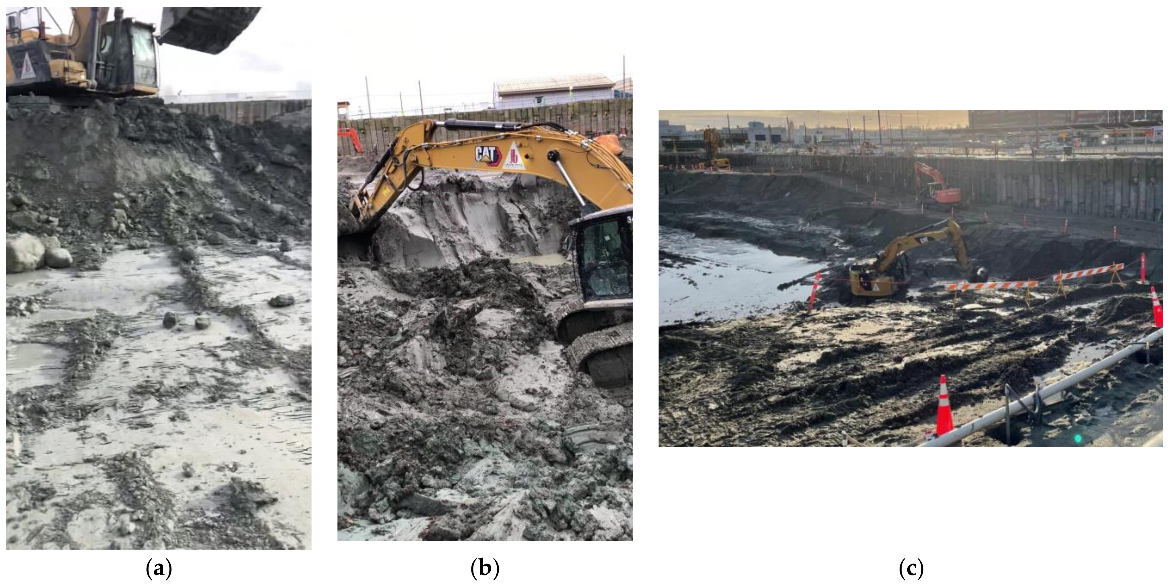
2S) during the preparation of a very large excavation (
Figure 1). The land on which the site was located was reclaimed from the shoreline at the beginning of the last century through the dumping of various materials [
3]. Emission of H
2S is known to occur in similar circumstances at the surface rather than following disturbance of covered material [
4,
5]. The shoreline was a mudflat at the time of reclamation containing detritus from intertidal colonization by plants and animals [
3]. Fill material included sawmill waste, demolition waste, branches and trees, garbage and trash, ashes from steam engines, and soil and rock excavated from other locations. Filled land extended to the original shoreline 1 to 2 km inland beyond the area of the excavation.
The fill material raised the height of the land to 5 m above sea level [
6]. The filled land is susceptible to liquefaction during earthquakes [
3]. Elevation above mean sea level is an important starting point in consideration of the excavation of fill material and the underlying original shoreline. The typical tidal water level at this location ranges from 0.5 m to 4.3 m [
7]. This migration is consistent with the previous comment concerning liquefaction [
3]. Tidal migration along the fill material could occur up to the maximum level of high tide, known as a ‘king’ tide. ‘King tides’ are recognized for causing damage to beaches and structures built on land whose elevation is below this level.
The filled land was used as a railway hub and the site of major industrial development in the surrounding area. The railway hub included a station and related infrastructure, a roundhouse and turntable for servicing locomotives, a powerhouse, a rail yard, and buildings that housed related operations [
3]. The railway station and related infrastructure were demolished and removed decades ago. A layer of gravel was applied to the top of the existing material to prepare it for use as a parking lot.
The soil in the excavation became progressively wetter with depth (
Figure 2). The material in the uppermost level was granular and fell easily from the bucket of the excavator. The first lower-level was wet and contained areas of ice. In the transition to the next lower-level, the soil became extremely plastic, like plasticine, and held the shape created by the action of the excavator. At the bottom of the excavation, the material became fluid-like with water. Materials of various colors were visible at the lower-levels. These were described as containing known contamination.
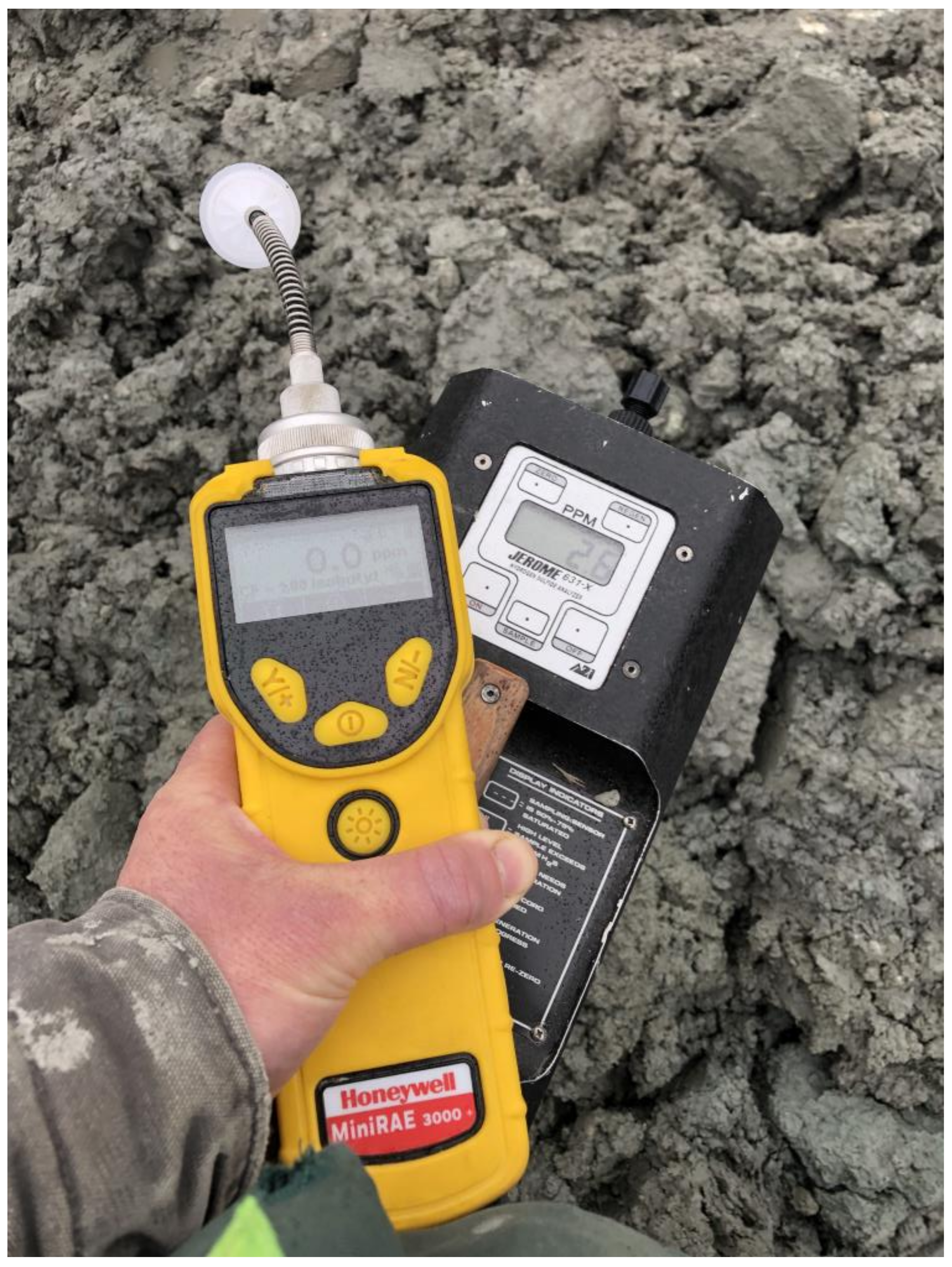
An odor recognizable as characteristic of rotting material at the ocean shore was detectable in this area. At the next lower-level, there was a faint odor of rotten eggs. The odor of rotten eggs is due to the emission of hydrogen sulfide (H2S). Workers commented that there seemed to be a relationship between the extent of wetting of the soil and the detection of the rotten egg smell. H2S was detectable by the nose but not by the instruments used by the excavation contractor for testing in this environment. The H2S sensor read zero.
The workers were fearful about continuing to work in this environment and raised this situation as a safety concern with their employer. Without an immediate and meaningful response, this situation would have led to the exercise of the right to refuse work due to the perception of the environment as unsafe.
This situation provided a rare opportunity to learn about this phenomenon and to determine its characteristics and significance in this circumstance and in the broader scope of excavations occurring under similar conditions. Anecdotal reports had indicated the occurrence of emissions of H2S in other excavations in the same area of the city. Unfortunately, these reports lacked quantitative information.
Questions that arise from this concern include:
What levels of H2S are encountered during activities intrinsic to this work?
What is the maximum level of H2S?
With what persistence do these emissions occur?
Can this work occur under normal conditions of operation without exceeding regulatory exposure limits for H2S applicable to workplaces? The answer to this question is currently unknown. The literature contains no information on which to base work strategy and, as necessary, the selection of respiratory protective equipment.
If exceedance of workplace regulatory exposure limits occurs, what modification(s) are necessary to address this concern?
Does this activity create environmental issues with nearby residential neighbors?
Surface soils can contain numerous gases and vapors [
8,
9,
10,
11]. Most common sources result from the disposal of organic chemical products into the ground, burial of vegetable and animal matter in garbage dumps, the filling-in of swamps and marshes, spillage and leakage from pipelines and tanks, and natural sources of petroleum located at or near the surface of the ground. Sulfur-containing substances are the source of H
2S and mercaptans.
The emission of methane from such sites is a well-known phenomenon that sometimes has lethal consequences [
12,
13]. Building codes require collection and venting systems under structures built in these locations. Occasional reports indicate the presence of high-level emissions from former industrial sites, such that monitoring during excavation is essential to prevent fire and explosion [
8,
9,
10,
11]. The migration of carbon dioxide has caused at least one documented fatal accident [
14].
H
2S is extremely toxic and has caused many workplace fatalities [
15]. For this reason, H
2S is one of the gases measured by 4-gas testers [
16]. These instruments read in ppm (parts per million). The situation reported here introduced confusion and potential distrust because workers smelled H
2S at a level in some locations describable as offensive and made the assumption that it was harmful based on previous education and training. Considerably complicating the situation was the fact that the odor threshold of H
2S is as low as 1 ppb (part per billion) [
17]. (1 ppm [part per million] = 1000 ppb).
Hence, a four-gas tester calibrated and performing correctly would not be able to detect H2S, even though it is detectable by the nose and can pose an offensive odor. Levels determined by this instrument less than 1 ppm (1000 ppb) pose no regulatory concern of exposure to workers, even though the nose clearly detects a progressively stronger odor up to the level of offensiveness. Detectability of odor does not necessarily equate to regulatory overexposure.
The regulatory exposure limit of H
2S in British Columbia, where this work occurred, is 10 ppm (parts per million), expressed as a ceiling not to be exceeded during the work shift [
18]. The basis for this level was to minimize the potential for eye and respiratory tract irritation, headaches, fatigue, dizziness, and effects on the central nervous system. Other jurisdictions use the Threshold Limit Value—Time-Weighted Average (TLV-TWA) recommended by the American Conference of Governmental Industrial Hygienists as the regulatory exposure limit. The current TLV-TWA is 1 ppm, averaged over 8 h [
19]. The basis of the current TLV-TWA is to prevent irritation in the upper respiratory tract and impairment of the central nervous system. The reason for decreasing the value from 10 ppm to 1 ppm was not explained.
2. Materials and Methods
A specialized instrument for H
2S, the Jerome 631-X (originally Jerome, later Ametek Arizona Instrument, and now AMETEK Brookfield, Chandler, AZ, USA), was obtained from a rental company [
20]. The Jerome 631-X measures down to 1 ppb. The rental company calibrated the instrument prior to use.
Appendix A provides further information about this instrument.
Typically, readings in workplace studies are obtained in the breathing zone [
21]. The breathing zone is an imaginary sphere with a radius of 0.6 m centered on the head from which a person obtains air during inhalation. The height of the breathing zone is 1.5 m. The instrument or sampling probe is positioned to obtain the reading from waist to shoulder height. An alternate sampling position is close (0.5 m) to the surface of the ground or the material under study. A principal reason is the absence of on-scale readings. This can occur outdoors because of surface air movement [
22,
23]. Surface air movement is continuous and can rapidly disperse emissions in the event of the absence of replenishment.
Sampling occurred outdoors through difficult weather conditions (temperatures around freezing, with rain and possible snow. Thorough sampling was essential in order to characterize emissions since little advanced information was available.
A video was recorded during the collection of each sample. Each video showed the context of the collection and the numerical value of each sample. The videos were stored in files organized by day and enable historic examination of the data should this become necessary.
In addition, emissions from contaminated soil posed a moving target because the focus of excavation is removal of soil and not continuous collection of samples containing little or no evidence of air contamination. The environment during excavation is constantly changing.
IHDA-AIHA (Industrial Hygiene Data Analyst-American Industrial Hygiene Association), published by Exposure Assessment Solutions Inc., Morgantown, WV, USA, and made available as a public service through the AIHA, was used for statistical analysis of the data. The emphasis here was first-pass decision-making rather than precision because the data were obtained under conditions of urgency with scarce resources rather than a disciplined, controlled study intended for academic-level research.
3. Results
During this investigation, teams of two excavators worked together to transfer material. The excavator at the lower-level removed material and passed this upward to the receiving level. The receiving level may have been intermediate between the bottom level and the mid-level such that material excavated from the receiving level was later passed upward to the mid-level. Loading of dump trucks by the second excavator occurred on the receiving level to which the first excavator passed the excavated material. The dump truck removed the material from the excavation for transfer to highway trucks for removal from the site. The process was repeated for the excavation of material from the space upward to the upper-level.
In order to position the instrument about 0.5 m above the surface of the material, the sample collector was required to crouch rather than stand normally. Hence, the sample collector was exposed to a level of H2S similar to that measured in the emissions from near the material’s surface. The approach has value since many of the emissions were near zero despite the presence of a detectable odor.
Measurement of area samples occurred at the height of the normal breathing zone, as noted.
The main investigation responded to findings during a preliminary walkthrough performed early in the process of deep excavation on the site. At the time of the walkthrough, two excavators were operating. One excavator was positioned in the deep area and was actively excavating material known to emit H2S when disturbed in this manner.
During the initial walkthrough, the instrument indicated the following levels of H2S: <1 ppm outside the excavation and part-way into the excavation, no odor; 1 to 4 ppb, a general area about 50 m from the area of known contamination, faint odor; 45 ppb, 10 m from the area of known contamination, strong odor; 190 ppb, 0.5 m from surface of known contamination, offensive odor.
This information indicated that no odor of H2S was detectable in areas unaffected by active excavation and that the instrument provided a reading of zero ppb at the same time. At some distance, the odor of H2S became faintly detectable by a nose, and the instrument started to read 1 ppb or higher. As the distance from the known source decreased, the odor and the reading on the instrument increased.
The level indicated by the instrument very close to the surface of known contamination of H2S was 190 ppb (0.19 ppm). This level was within the region of concern of jurisdictions that use the TLV-TWA of 1 ppm averaged over 8 h as the regulatory exposure limit. In addition, the level of emission achievable by the contamination during large-scale excavation and materials handling, and hence the level of concern to be applied, were unknown. Emission of H2S based on the sampling reported above and in discussion with operators of excavators and other equipment positioned in the excavation was related solely to the disturbance of material. The elevation at which the emission occurred was potentially at or below the level of the original shoreline. Hence, the emission was a consequence of the location and depth of the excavation on the former shoreline, and the chosen means of raising the level of the land through use of readily available materials susceptible to microbial degradation.
This situation posed many questions for which there were no answers. In order to respond to worker concerns and to characterize the emissions to a level of predictability, this investigation necessitated many repetitions in different locations over a period of several weeks. A large number of measurements was believed to be necessary because the occurrence, duration, and upper limits of the emissions were unknown. The literature provided no precedents on which to set sample numbers sufficient to gain confidence in what could occur. Experience gained from large numbers of repetitions showed the wisdom of this approach.
Another unknown was knowledge of all of the sources of H2S on the site. The preliminary measurements established the concern about depth. The potential for emissions at shallower depths from other sources was unknown.
Table 1 contains results from the sampling for H
2S on the site of the excavation. The table is organized by elevation of the level within the excavation, by activity, and by day. Large-scale unexpected emissions sometimes occurred during excavation and during transfer to a higher level for loading onto trucks. These were superimposed into groups having consistent low-level values. High levels of unpredicted emissions were separated from routine levels to better determine the impact of these unexpected events on the low-level background.
An important consideration when emission occurs on a worksite is the potential for transfer off-site into the surrounding community. Sample Groups 1 to 10 obtained at the boundaries between the worksite and the non-involved area of the property were low in magnitude compared to those obtained in areas where the work activity was occurring. The closest contact with the community occurs at about 100 m distance on the west side of the excavation. Hence, the detection of odor off-site was very unlikely.
Sample Group 21 highlights the influence of the work activity on the level of emission. Sample Group 21 was obtained in an area of active excavation just as work stopped at the end of the shift. Emission of H2S decreased rapidly to background levels for the site soon after cessation of work activity.
The distribution of measured values was predominately arithmetic compared to the lognormal distribution typically observed in workplace exposure data [
21]. This would suggest that the system under study was chaotic compared to one strongly oriented to the normal or lognormal distribution.
The highest recorded levels of emission of H
2S (
Figure 3) occurred during excavation of material from the bottom of the excavation (Sample Groups 13 to 15, 19 and 20, and 28 and 29). A second high-level, apparently unrelated source was detected during excavation on the upper-level (Sample Group 35). The values in these Sample Groups reflected intent to determine the maximum level of emission of H
2S that could occur from material excavated from this site.
Levels measured from freshly exposed material caused the maximum possible exposures that could occur on this site. As a result, the sample collector was the most heavily exposed worker on this site. Operators of equipment were ~10 m distant from the point of emission. Hence, the exposure of workers performing routine activity was considerably lower than that experienced by the sample collector.
Sample Groups 11 and 12, 13 to 15, 16 to 18, 19, 20, 22 to 27, 28 and 29 highlight the extent of the variability in the emission of H
2S from material excavated from the bottom level. The emission from some newly exposed surfaces was very low, while that from others was very high (
Figure 3).
Figure 4 shows the highest level of emission (2600 ppb). The change in magnitude of emissions was unpredictable both in occurrence and duration. High-level emissions decreased rapidly once disturbance by the excavator ceased.
Emission at the levels reported in Sample Groups 13 to 15, 19, 20, 28, and 29 was sufficiently high to activate concern in some jurisdictions relative to the regulatory exposure limit of 1 ppm expressed as an 8-h time-weighted average. Experience gained during sample collection indicates that high levels of possible regulatory interest are transitory.
Emissions from Sample Group 35 suggest that materials capable of emitting H2S can be present at any level in the fill material. This also highlights the need for a more thorough investigation of possible sources of emission based on site history. To illustrate, wastewater (sewage) handling is a possible issue at this site because of the former railway station and the concentration of people using the facility. Demolition waste present in the upper-level of the fill could emit H2S for this reason.
The installation of a sewer line as part of the redevelopment of the site illustrates this concern. The depth of sewer installations is typically 2 to 3 m below the surface. This would put the depth of the excavation into the mid- to upper-level of the soil profile. Emissions in sample group 44 suggest the presence of a source of the emission of H2S in the upper-level of the soil profile, where demolition waste from the former use of the site would be expected.
4. Discussion
This article discusses a situation that occurred during the excavation of disturbed soil in a construction site located on a former tidal mud flat. Excavation initiated the unexpected emission of H2S from deposits of biological material in the soil.
Anticipation and recognition of the issue posed by H2S combined with information concerning the depth of the excavation compared to the depth of contamination identified in core sampling, the height of the tide, and starting elevation of the original surface of the land are essential for determining the initial strategy of excavation and choice of instrument(s) used for monitoring.
The profile diagram (
Figure 4) combines the distribution of the disturbed material with elevations relevant to the excavation and sea level. The depth of the excavation in relation to sea level shows the relationship between the absence of emission of H
2S and where it can be expected based on the elevation of the former shoreline relative to the depth of the excavation. Any disturbance, especially puncturing of the intertidal layer, should be expected to produce H
2S. In addition, any organic material dumped onto the intertidal layer as fill potentially contributes to the emission of H
2S. This information alerts site managers about the potential for the emission of H
2S from these sources. It provides the advance time needed to respond to it by obtaining a monitoring instrument of the type used in this investigation.
The introduction posed questions of fundamental importance regarding potential exposure of workers in the excavation. Visual inspection of
Table 1 indicates that the levels of H
2S during the vast majority of routine activity ranged from 0 ppb to 25 ppb based on samples lasting 1 min each. Using the upper-level of 25 ppb and assuming a constant average concentration over the work shift of 8 h and the TLV-TWA of 1 ppm (1000 ppb) as the regulatory exposure limit, the dose would be (25 ppb)/(1000 ppb) × 100% = 2.5% of the permitted dose. This calculation is extremely conservative and shows that the calculated dose is a small fraction of the permitted dose.
The statistics involved with dose calculations indicate that exceedance of the TLV-TWA in this situation is highly unlikely for doses that are low compared to the action level of 500 ppb. (The action level is 50% of the TLV-TWA) [
24,
25].
Regarding the high-level emissions recorded during initial exposure to material containing H2S, they rose rapidly to a peak and decreased rapidly thereafter. Based on readings obtained during this phenomenon within the context of the accompanying videos, the duration of the emission was less than 10 min. Within the days during which these abnormal emissions occurred, the frequency was once per day. Integrating the previous calculation with the occurrence of one episode of 10 min at 2600 ppb (the maximum recorded level), the Time-Weighted Average concentration would be [(470 min × 25 ppb) + (10 min × 2600 ppb)]/(480 min) = 79 ppb. The dose would be (79 ppb)/(1000 ppb) × 100% = 7.9% of the permitted dose. This level of dose is extremely conservative because of the distance between the operators of equipment and the point of emission.
As in the previous example, the statistics involved with dose calculations indicate that exceedance of the TLV-TWA is highly unlikely for doses that are low compared to the Action Level of 500 ppb in this situation. (The Action Level is 50% of the TLV-TWA) [
24,
25].
Hence in both cases, the measurements and the associated calculations support the hypothesis that work in this environment will not overexpose operators of excavators and others who do not approach freshly exposed surfaces of emission closely. This investigation provided tremendous benefit on-site by characterizing emissions of H2S and identifying the possible source(s) beyond those identifiable at first glance, and alleviating worker concerns.
The emission of H
2S from the materials excavated from the site poses questions of fundamental importance concerning the mechanism of formation and emission. The H
2S molecule is formed by the action of bacteria through anaerobic respiration. Sources of S can include S-containing amino acids and sulfates. Both pathways are possible but depend on different bacteria [
26].
Sources containing sulfur atoms in this situation include plants and detritus deposited on the original shoreline [
26,
27]. Workers commented about the odor of a shoreline on this site at the bottom of the excavation. Additional possible sources include trees and branches, wood and wood waste, garbage and trash, and sewage from on-site disposal. While these materials could have been present in all levels of the excavation, experience showed that almost all were present only at the bottom level at or slightly above sea level and at the upper-level in the debris containing demolition waste.
Covering these materials with earth excluded contact with oxygen and permitted only anaerobic respiration. Contact with water occurred through downward seepage of rain from above and horizontal seepage of tidewater and groundwater. Aerobic and anaerobic bacteria grow in the space between soil particles [
26]. This growth requires water. The H
2S is trapped in the water in the particle spaces.
The emission of H2S was not detectable until disturbance occurred. The action of removing the material disturbed the status quo through force induced by mechanically induced movement. Disruption of the status quo was linked to the emission of H2S from the material. The material that was off-gassing was plastic and retained its shape or was very wet to the point of liquefaction. Emission ceased soon after the disturbance ceased.
Emission of the type described here occurs in shear-thinning, pseudo-plastic, non-Newtonian fluids [
28,
29,
30,
31]. Shear-thinning, pseudo-plastic, non-Newtonian fluids trap gas and release it to the atmosphere on the application of a shear force. Emission ceases soon after cessation of application of the shear force. Paint, which behaves in this way due to deliberate formulation, is a shear-thinning, pseudo-plastic non-Newtonian fluid. Stirring applies the shear force. The viscosity decreases and the liquid flows. The viscosity restores once stirring ceases.
In the case of non-Newtonian fluids trapping gases, application of a shear force, such as rotation of the impeller of a pump reduces the viscosity and enables escape of the gas to the atmosphere [
30]. Prior to application of the shear force, emission of gas may not have occurred. Emission ceases rapidly once rotation of the impeller ceases.
This is not to suggest categorically that the emissions occurring in this situation were the result of applying a shear force to a non-Newtonian fluid. However, there are many similarities between the behaviors observed during this investigation and behaviors known to occur in non-Newtonian fluids [
28,
29,
30].
pH is another factor that influences emission. H
2S can ionize to form HS
− and S
2− ions. Ionic forms of H
2S are reservoirs for the storage of sulfur [
30]. Reactions involved in the formation of HS
− and S
2− are readily reversible. This reversibility depends on changes in pH. This process enhances the storage of H
2S in this environment as it does in normally recognized watery environments. Change in pH is not likely to be a factor in this situation.
5. Conclusions
The unpredicted and unexpected emission of H2S from material near the bottom of an excavation posed a serious perceptual issue to operators of the equipment. These emissions originated in material related to the former shoreline underlying the site and possibly to fill material used to raise the level of the ground. Emission appears to be related solely to the disturbance of this material. That is, emission occurred rapidly following the disturbance and diminished rapidly to an ambient level once the disturbance ceased. The ambient level in the absence of disturbance was <1 ppb and not detectable by a nose. Testing using an appropriate monitoring instrument was able to demonstrate that exposure during work in the excavation was low relative to regulatory exposure limits. The thoroughness of the investigation showed quantitatively the imposition of high levels of emission of H2S from freshly disturbed material onto predictable background levels. This investigation also established the lack of predictability of emission from one bucketful of fill material removed by the excavator to another. This result established the need for the collection of as many samples as practicable in order to establish the status quo of the situation. The approach taken during this investigation also addressed, clarified, and resolved concerns expressed by affected workers. This investigation showed the importance of the profile diagram for anticipating the emission of H2S when excavation occurs over a former ocean shoreline. The profile diagram integrates the starting elevation of the filled land, the water table, mean sea level, occurrence of contamination, types of soil, and the depth of the excavation. In this way, construction management can anticipate the emission of H2S whenever the depth of the excavation penetrates through the elevation of the former shoreline. The findings from this investigation have potential importance and application worldwide in this type of work.


