Abstract
This work presents the development of a decision-making strategy for fulfilling the power and heat demands of small residential neighborhoods. The decision on the optimal operation of a microgrid is based on the model predictive control (MPC) rolling horizon. In the design of the residential microgrid, the new approach different technologies, such as photovoltaic (PV) arrays, micro-combined heat and power (micro-CHP) units, conventional boilers and heat and electricity storage tanks are considered. Moreover, electricity transfer between the microgrid components and the national grid are possible. The MPC problem is formulated as a mixed integer linear programming (MILP) model. The proposed novel approach is applied to two case studies: one without electricity storage, and one integrated microgrid with electricity storage. The results show the benefits of considering the integrated microgrid, as well as the advantage of including electricity storage.
1. Introduction
In the traditional electrical grid, power is generated in large, centralized plants and then transmitted to the end-user using one-directional flows [1]. The need to meet the challenges and targets regarding energy savings and environmental protection lead to an increase in interest in the use of technologies such as smart grids [2,3,4,5], distributed energy resources [6,7,8], as well as the need for the development of new management structures [9,10,11,12,13,14] for the resulting systems. In addition to generation units, distributed energy resources (DER) systems may also include storage and transmission capacities, as well as infrastructure for the connection and control of the use of all the installed technologies [15]. DER systems have many advantages in terms of the increase of power quality, production of energy close to demand, high-energy utilization, and decrease of dependency on fossil fuels, but their intermittency is a major disadvantage [16], especially since generation and demand tend to be mismatched, resulting in wasted energy [17] or challenges in the microgrid operation, among other issues [18,19]. Structural optimization techniques are typically used for the optimal design of DER systems [20,21,22,23,24,25]. The operational optimization and control of the DER system become challenging tasks due to the integration of many different technologies (photovoltaics, combined heat and power, wind turbines, etc.) in a single system, as well as due to the uncertainty and variability problems of these energy sources.
These issues bring many complications for the operators, which try to manage and control complex or multi-microgrids with limited fast-ramping resources, in order to maintain the flexibility of the power system [10]. The management of an energy system such as a microgrid encompasses both supply and demand side management to satisfy network constraints with the goal to achieve reliable, sustainable and economical operation [26].
Microgrids are capable of operating either in grid, connected, or autonomous operation mode during a faulted situation, yet their stability, reliability, and operational control is more challenging during the islanded mode [27,28].
In traditional hierarchical control architectures, the control model has three levels [29]: the primary control, responsible for load sharing and for maintaining stability and autonomous operation, the secondary control, which restores the voltage/frequency offsets introduced by the primary control, and the tertiary control level, to calculate the optimal references for the microgrid sources based on economic objectives. Modern architectures utilize approaches ranging from decentralized and distributed multi-agent [30,31], bilevel programming and reinforcement learning [28], fuzzy logic [32], or genetic algorithms [33] for control and coordination purposes.
Among the different control approaches, the model predictive control (MPC) has been proved satisfactory for intelligent control of DER systems and superior to standard control methods [34,35,36,37]. The MPC strategy is based on a discrete-time model of the system, which is used for the prediction of the behavior of the system during a future control horizon as a function of the manipulated variables [38].
MPC is currently a popular control methodology for industrial and process applications, largely due to its inherent ability to efficiently handle constraints in multivariable dynamical systems [39]. It comprises characteristics such as optimization of power flow in the microgrid, incorporating the costs of generation and operation of the DER systems as constraints [28]. The rolling (or receding) horizon concept has been broadly used in control methods as a means to deal with control problems when a cost function has to be minimized in a given time horizon. The method solves the optimization problem with a sequence of iterations, each of which models only part of the horizon in detail, while the rest is represented in an aggregate manner [40].
Based on these characteristics, an MPC strategy based on the rolling horizon concept has the potential to achieve the global solution of the cost function over a specified period of time, while also being able to acquire sufficient information on future conditions [41]. Thus, this will enable improved decision-making in the design, operation, control, and planning of the DER system.
In the following sections, the development of a new MPC-based decision-making strategy is presented, based on the concepts discussed in [42]. Thus, the formulated optimization problem includes various constraints for the selection of the optimal values of the manipulated variables over the control horizon. From the optimal solution, only values corresponding to the first time interval are used and the problem is reformulated and solved in the next time instance following the rolling horizon concept. The main objective of the approach is to ensure the network is able to meet the energy (in terms of electricity and heating) demand of the consumers in addition to minimizing the overall cost.
The approach offers flexibility in terms of the number and type of energy generation solutions that are included, the size and location of the network and the demand type (e.g., electricity, heating) and profiles that can be considered. It offers the capability to quickly asses the network at high level, without the need of rigorous modelling of the DER technologies.
2. Problem Statement
A residential neighborhood consists of a number of dwellings with estimated electricity and heating profiles. Every dwelling satisfies its demands through a combined heat and power (CHP) plant, a photovoltaic (PV) array, electricity storage, and a back-up boiler. The CHP plant, operated using natural gas, and the PV array are used to meet the electrical demand. The high-temperature exhaust of gas of the CHP plant and the supplementary boiler are used to accommodate the thermal load. Surplus electricity can be delivered back to the grid, while the utility electricity can support the deficit. Electricity can be transferred between the various dwellings in the residential network in two different ways: through the existing power transmission network or using central storage capacity. In this case, energy produced in surplus is stored, and transferred to the dwellings when demand increases. There is also the possibility of heat exchange between dwellings through a heating piping network.
For the MPC optimization problem, the following data are given (Figure 1), as presented in [42]:
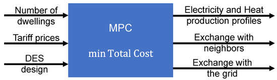
Figure 1.
Inputs and outputs of the MPC optimization problem.
- The number of dwellings and their electricity and heat profiles for the prediction horizon
- Electricity and gas tariff prices, prices for selling excess electricity
- Allocation and capacity of DER technologies
- Storage capacities
- Initial values for all state variables
The objective function to be minimized includes all the components that affect the operational cost of the DER system over the prediction horizon: the cost of electricity purchased from the grid, the cost of the fuel consumed, as well as the environmental cost. The heat and electricity storage terms are accounted as well, as an addition to the model presented in [42]. Furthermore, the revenue from selling the surplus electricity back to the grid is also considered in the calculation of the DER network operational grid.
The solution of the resulting optimization problem provides optimal values for the decision variables over the rolling horizon. The key decision variables considered are:
- The electricity and heat generation profiles for each individual dwelling within the network
- The heat transferred between dwellings through the pipeline network
- The electricity transferred between the dwellings and between the dwelling and the grid
2.1. Mathematical Model
A mixed integer linear programming (MILP) formulation is considered for the MPC problem, which is solved during each time period of the operation of the network.
2.1.1. Objective Function
The objective of the problem is to minimize the total operational cost for the DER systems over the prediction horizon, and includes a revenue component and a cost component. The operation of the microgrid is partitioned into equidistant time periods. The revenue component of the objective function includes the income from selling electricity to the grid. The cost component includes the cost of purchasing electricity from the grid, the cost of the consumed fuel in the various energy generation units, the operational and maintenance cost of the different generation technologies, as well as the environmental cost. Furthermore, as an addition to the model described in [42], the heat and electricity storage terms are included in the objective function.
Thus, the objective function is formulated as follows:
The total cost for purchasing electricity is calculated using Equation (2), through the cumulative amount of electricity purchased multiplied by the utility electricity rate:
The environmental cost of the network operation is determined by the cost for carbon emissions (based on the carbon content of the purchased electricity and natural gas) and is calculated using Equation (3):
The income from selling electricity is determined by the cumulative amount of electricity delivered to the grid from the excess generated by the CHP units multiplied by the electricity buy-back price:
The operational cost of the CHP units includes the fuel cost, which is calculated based on the cumulative fuel consumption for each period multiplied by the fuel price:
The operational cost of the back-up boilers is composed of the fuel cost, calculated by the cumulative fuel consumption for each time period multiplied by the fuel price:
The operational and maintenance cost of the heat and electricity storage is calculated from the cumulative heat energy or electricity, respectively, multiplied by a unit maintenance cost coefficient as expressed in the following equations:
2.1.2. Supply–Demand Relationships
A balance of supply and demand has to be achieved for both heat and electric power at each time instance. Electricity demand can be met through purchase from the national grid, generation from the PV arrays and CHP units installed in the microgrid, as well as the power transmission network between the dwellings, and electricity available from storage. Heat loads can be satisfied by conventional boilers, CHP units, heat stored in the storage tanks, and by transferring heat among the dwellings through the heating pipeline network.
Equation (9) presents the relationships for the electric power, while Equation (10) shows the relationship considered for the heat:
where HER is the heat to electricity ratio.
2.1.3. Grid Interaction Constraints
Additionally, further constraints are added to the model in order to set to prevent buying and selling energy at the same time during the network operation:
where M is an appropriate upper bound.
2.1.4. CHP Unit
Equations (13) and (14) link the binary variables that describe the operation of the CHP units. The binary variable takes the value of 1 only when the CHP unit i starts up, while variable takes the value 1 only when the unit shuts down.
Equation (15) forces the CHP unit i to be functional for at least time periods after start-up:
The following set of equations ensure that a CHP unit is in operation, but still at start-up mode for at least time periods after the start-up. The start-up mode implies that, although the unit consumes gas, it is not delivering electricity or heat:
Equation (17) forces the CHP units to be out of operation for at least time periods after shutdown:
The performance characteristics of the CHP plant are defined in Equation (18). This indicates that the CHP unit cannot generate more energy than its installed capacity when it is in operation and not in start-up mode. Furthermore, a lower bound on CHP electricity generation is enforced:
Equation (19) indicates that if the unit is in start-up mode, no electricity is produced:
2.1.5. Back-Up Boiler
The performance characteristic of the back-up boiler is determined using Equation (20). Its purpose is to prevent the unit from exceeding its rated capacity:
2.1.6. Heat Storage Tank
Additional constraints are needed to ensure the operation of the heat storage tank. Equation (21) describes the heat inventory balance constraint. It states that for each storage tank the total amount of stored heat at the end of a time period is equal to the heat stored at the end of the previous period plus the recovered heat diverted towards storage minus stored heat that is released to meet heat demand, during that time period:
Equation (22) ensures that the heat stored in the storage tanks is within the tank capacities at all times:
Equation (23) forces the heat stored in each storage tank at the end of the control horizon to be equal to the initial level:
The difference in heat stored in each storage tank between two consecutive time periods is constrained by the following inequality:
with and percentages of the maximum heat storage.
2.1.7. Electricity Storage
The electricity inventory balance is described by Equation (25), similarly to the heat storage balance equation. The electricity storage is assumed to be a lead-acid battery with a charge (cl = 10%) and a discharge loss (dl = 15%), respectively.
Equation (26) forces the electricity stored at the end of the control horizon to be equal to the initial level. Moreover, Equation (27) poses an upper bound on the stored level
The difference in electricity stored in the central storage between two consecutive time periods is constrained by the following inequality:
with and percentages of the maximum electricity storage.
2.2. Illustrative Example
In order to demonstrate the application of the decision-making strategy described in the previous section, a case study of a DER network is considered, with the main focus on the Greek residential sector, comprised of 10 buildings in Athens (Greece).
The full calendar year is divided into three seasons [42]: summer (June–September), mid-season (March–May, October), and winter (November–December, January–February). Furthermore, the day is divided into six periods: p1 (07:00–09:00), p2 (09:00–12:00), p3 (12:00–13:00), p4 (13:00–18:00), p5 (18:00–22:00), and p6 (22:00–07:00).
The residential electricity and heat demand profiles of the 10 dwellings have been created based on the consumption of an average Greek household [43], and defined to have the resolution of one hour. The electricity and gas tariff prices reflect the Greek reality [24].
Table 1 presents the data on solar irradiance, while the heat and electricity loads are illustrated in Table 2 and Table 3, respectively.

Table 1.
Solar irradiance [24].
Table 2.
Heat loads for the 10 dwellings [24].
Table 3.
Electricity loads for the 10 dwellings [24].
The technical characteristics of the DER technologies considered for this case study are taken from the technical datasheets available from the producers and presented in Table 4 for the CHP units and in Table 5 for the other technologies, respectively.
Table 4.
Capacity, cost, and technical characteristics of the CHP units.
Table 5.
Capacity, cost, and technical characteristics of other units.
The operational cost of the CHP units is the cost of purchasing the fuel (natural gas) for operating the unit.
The utility rate is 0.11 EUR/kWh, while the price of selling electricity to the grid is 0.08785 EUR/kWh for the CHP units, and 0.55 EUR/kWh for the PV units. This price refers to the electricity buy-back price based on Greek governmental policies for PV systems up to 10 kWp and for CHP systems based on Greek data [24]. The cost of natural gas is assumed equal to 0.054 EUR/kWh. The carbon tax is 0.017 EUR/kg. The emission of CO2 for every kWh produced is 0.781 kg/kWh, while for every kWh of natural gas is 0.184 kg/kWh.
The electricity factor refers to the end-use energy produced by the Greek electricity power mix, while the natural gas factor is based on the lower heating value (LHV) and refers to kWh of input fuel.
More information on the other input data used, as well as the nomenclature can be found in Appendix A, Appendix B and Appendix C.
3. Results and Discussion
Following a rigorous design methodology [22], the capacity determined for each of the 10 dwellings (i1–i10) in the network is shown in Table 6.
Table 6.
Installed capacity of units.
Additionally, a central electricity storage tank of 100 kWhe is installed. Furthermore, electricity is exchanged between the buildings and the power transmission network.
The MPC problem defined in the previous sections is solved for a time period of four days (winter season) using a rolling horizon of 96 1-h time intervals (i.e., a rolling control horizon of 12 h), as shown in Figure 2.
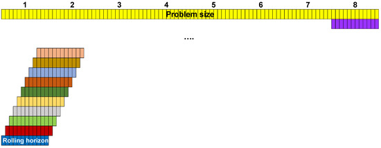
Figure 2.
Rolling horizon approach.
The problem is formulated as an MILP model, which is implemented and solved in GAMS [44], using the CPLEX 11.1.1 solver, to global optimality. The average time to solve the MILP problem is 0.2 s. The runs are performed on a regular PC running at 2.53 GHz. Due to the action horizon being equal to 1 h, the size of the system can be considerably scaled-up before running into intractability problems. However, for solving very large-scale problems, distributed MPC algorithms need to be used.
To investigate the potential saving costs when an integrated microgrid scenario is considered, two system options have been analyzed:
- (a)
- An integrated microgrid with no central electricity storage
- (b)
- An integrated microgrid case with central electricity storage.
Furthermore, to better assess the integrated microgrid, the operation of a baseline DER network which considers no storage capabilities, and without using the MPC approach discussed above, is investigated. The total cost obtained for this baseline scenario is EUR 1430.20. The further breakdown of the total cost for the three scenarios considered is presented in Table 7.
Table 7.
Cost breakdown for the different scenarios considered.
As shown in Table 7, the integrated DER network with central electricity storage achieves savings in the total cost of 300% compared to the baseline, and 11.5% compared with the microgrid without electricity storage. This is mainly due to the fact that when central electricity storage is available, the operational cost of the CHP unit is lower (the CHP units operate for less time, while the electricity storage serves the electricity loads).
In terms of the breakdown of the costs, the two integrated microgrid scenarios do not differ significantly, with the exception of the income from selling electricity to the grid. Compared to the baseline, this income leads to negative values in the total cost for the integrated scenarios, making the operation more economical. Moreover, both microgrids have significant reduction of the operational (>50%), environmental (>90%), and purchase of electricity from the grid (>85%), with an increase in income of >3700%.
As the behavior of the different households during the microgrid operation are similar, to illustrate the typical behavior of the households, Figure 3, Figure 4 and Figure 5 show the state of one building (i1) over the 4-day time horizon in the case of the integrated microgrid with electricity storage.
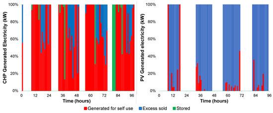
Figure 3.
Operation of the CHP and PV unit, respectively, over the 4-day time horizon for household i1.
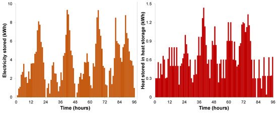
Figure 4.
Evolution over the 4-day time horizon of the central electricity and heating storage content, respectively, for household i1.
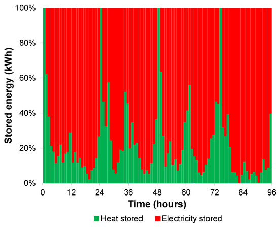
Figure 5.
Split of energy stored between electricity and heating storage.
Figure 3 illustrates the operation of the CHP and PV unit, respectively, as well as the distribution of the produced electricity among self-use, electricity sold to the grid, and electricity sent to storage. The results show that the CHPs are in operation for most time steps, and most of their energy is used internally. Excess electricity is sold to the grid for the periods in which no storage is required. In the case of the PVs, for the majority of time steps they are in operation, the electricity produced is sold to the grid. Moreover, when the demand is high, and the CHP units are not able to produce sufficient energy to cover this, the electricity generated from PV is utilized internally.
Figure 4 shows the state of the heat and electricity storage during the 4-day time horizon investigated, respectively. The electricity is being stored during most time steps, enabling a decrease of the cost by reducing the amount being purchased from the grid. This behavior is already observed in the cost breakdown in Table 7. Furthermore, although most stored energy goes into the electricity storage (Figure 5), the presence of both storage options ensures flexibility in operation. Thus, most of the energy not being used or sold can be available for later time steps, when the demand exceeds supply, and as such reducing the reliance to satisfy demand from the national grid.
Finally, Figure 6 represents the electricity exchange with the grid. As expected, for the periods in which the system does not purchase electricity from the grid, the excess energy is exported, ensuring the profitability of the integrated DER systems design. For the scenario when the network has storage available, the amount of electricity purchased is lower and more excess electricity is being sold compared to the other scenarios considered (as the cost breakdown in Table 7 illustrates).
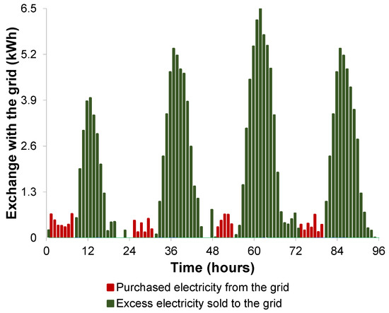
Figure 6.
Evolution over the 4-day time horizon of the electricity import and export for household i1.
4. Conclusions
In this paper an MPC rolling horizon approach is proposed for the development of a decision-making strategy for the optimal operation of a microgrid system designed to satisfy the energy (in terms of electricity and heating) demand for a residential network. The problem is formulated as an MILP model, which optimizes an objective function defined as the total cost of the microgrid. This cost includes investment, operating and maintenance, and environmental costs. The possibility of exporting energy to the national grid is considered, and the income made in this way is also considered in the total cost of operating the microgrid.
Based on this methodology, a generic model is developed, which includes multiple flexible components for the generation of energy (CHPs, PVs, boilers), as well as electricity and heating storage options. Furthermore, there is the possibility of satisfying the heating demand by transferring heat among the dwellings through a heating pipeline network. Model inputs are the electricity and heating demands, respectively, for each of the individual dwellings, the solar insulation, as well as the capacities of the different generation and storage units.
In order to assess the benefits of the approach, two system designs have been examined for a residential network formed of ten dwellings. In the first case, the renewable energy integrated microgrid considers no electricity storage available, while for the second, the DER systems have electricity storage. The results clearly illustrate the advantage of the integrated microgrid case, which has a lower total and operational cost (up to 300% reduction for the network with electricity storage). The increased income from selling to the grid enables the network to make a profit. Furthermore, for the scenario where storage is considered provides higher flexibility to the system, albeit with a slight (+9%) increase in the environmental cost.
Further improvements could consider different import and export prices for the energy exchanged with the grid [45]. Thus, the benefits of the presence of the storage options could be further explored by ensuring these exchanges are done in an optimal way. More realistic relationships can be used to describe the performance of the renewable energy technologies (e.g., variation of efficiency of generation units at part-loads [46,47], defining alternating power function and state of charge for storage systems [28,48]), or using clustering techniques to select typical operating periods [49,50].
Impact of national policies towards adoption of renewable energy generation, such as feed-in-tariffs or renewable heat incentives [51], must be included in the modelling of the DER system.
The residential neighborhoods do not consume only heating and electricity. Future models must include other typical needs of the consumers, such as domestic hot water or cooling [52], according to their specific location. Additionally, candidate technologies to answer to these demands, as well as new solutions for heating or electricity (e.g., biomass boilers, wind turbines, air conditioning units, adsorption chillers) will provide sufficient options to satisfy them.
Moreover, the uncertainty on the input variables (e.g., solar irradiance, energy demands) should be considered in the modelling of the residential DER network [19]. This will enable investigating the impact of these uncertain variables on the primary output (the total cost) and improve the design and their overall planning and performance.
The utilization of blockchain technologies in the transfer of excess energy produced using renewable resources between the households, as well as between the households and the national grid, will further enhance the DER system [53], not only in terms of impact on cost, but on the security of the network and transactions as well.
Finally, as all the elements above are included in the models, and as the size of the network moves from test cases of 5–10 dwellings to real neighborhoods, speed-up of the computational times is needed. Thus, network management systems based on MPC could provide automation and results in real-time for the operation of the DER systems.
Author Contributions
Conceptualization, E.M., B.D., and H.A.-G.; methodology, E.M.; software, E.M. and B.D.; formal analysis, E.M. and B.D.; investigation, E.M. and B.D.; resources, E.M. and H.A.-G.; data curation, E.M. and B.D.; writing—original draft preparation, E.M. and B.D.; writing—review and editing, E.M., B.D., and H.A.-G.; visualization, E.M. and B.D.; project administration, E.M. and H.A.-G.; funding acquisition, H.A.-G. All authors have read and agreed to the published version of the manuscript.
Funding
This research has no external funding.
Institutional Review Board Statement
Not applicable.
Informed Consent Statement
Not applicable.
Data Availability Statement
Not applicable.
Conflicts of Interest
The authors declare no conflict of interest.
Appendix A. Specification of Cost Terms
| PV investment cost (EUR) | |
| Boiler investment cost (EUR) | |
| CHP investment cost (EUR) | |
| Operational and maintenance cost of PV (EUR/year) | |
| Operational and maintenance cost of boiler (EUR/year) | |
| Operational and maintenance cost of CHP (EUR/year) | |
| Total cost for purchased electricity (EUR/year) | |
| Total environmental cost (EUR/year) | |
| Income from selling electricity to the grid (EUR/year) |
Appendix B. Input Data
| Natural gas price (EUR/kWh) | 0.054 | |
| Interest rate | 0.075 | |
| Carbon intensity of electricity (kg CO2/kWh electricity) | 0.781 | |
| Carbon tax of CO2 (EUR/kg CO2) | 0.017 | |
| Carbon intensity of natural gas (kg CO2/kWh natural gas) | 0.184 | |
| Regulated tariff for electricity purchases (EUR/kWh) | 0.11 | |
| Capital cost of PV (EUR/kW) | 4140 | |
| Capital cost of boiler (EUR/kW) | 100 | |
| Project lifetime (years) | 20 | |
| Electrical efficiency of the PV unit | 0.12 | |
| Thermal efficiency of the boiler | 0.80 | |
| Price of selling excess electricity from PV unit (EUR/kWh) | 0.55 | |
| Price of selling excess electricity from CHP unit (EUR/kWh) | 0.0875 | |
| Capital cost of the heat storage tank (EUR/kW) | 25 | |
| Heat loss coefficient of the heat storage tank (kWh lost/hour) | 0 | |
| Operational and maintenance cost of the heat storage tank (EUR/kWh) | 0.001 | |
| Capital cost of the electricity storage tank (EUR/kW) | 415 | |
| Operational and maintenance cost of the electricity storage tank (EUR/kWh) | 0.01 | |
| Charge loss of the lead-acid battery | 0.10 | |
| Discharge loss of the lead-acid battery | 0.15 |
Appendix C. Binary Variables
| 1 if dwelling may sell excess electricity to the grid at period ; 0 if it may buy from the grid | |
| 1 if the CHP unit in dwelling is in operation during period ; 0 otherwise | |
| 1 if the CHP unit in dwelling shuts down in period ; 0 otherwise | |
| 1 if the CHP unit in dwelling starts up in period ; 0 otherwise | |
| 1 if the CHP unit in dwelling is in operation by still in start-up mode during period ; 0 otherwise |
References
- Qi, W.; Liu, J.; Christofides, P.D. Distributed supervisory predictive control of distributed wind and solar energy systems. IEEE Trans. Control Syst. Technol. 2013, 21, 504–512. [Google Scholar] [CrossRef]
- Eltigani, D.; Masri, S. Challenges of integrating renewable energy sources to smart grids: A review. Renew. Sustain. Energy Rev. 2015, 52, 770–780. [Google Scholar] [CrossRef]
- Kakran, S.; Chanana, S. Smart operations of smart grids integrated with distributed generation: A review. Renew. Sustain. Energy Rev. 2018, 81, 524–535. [Google Scholar] [CrossRef]
- Farmanbar, M.; Parham, K.; Arild, Ø.; Rong, C. A widespread review of smart grids towards smart cities. Energies 2019, 12, 4484. [Google Scholar] [CrossRef] [Green Version]
- Dileep, G. A survey on smart grid technologies and applications. Renew. Energy 2020, 146, 2589–2625. [Google Scholar] [CrossRef]
- Akorede, M.F.; Hizam, H.; Pouresmaeil, E. Distributed energy Resources and benefits to the environment. Renew. Sustain. Energy Rev. 2010, 14, 724–734. [Google Scholar] [CrossRef]
- Allan, G.; Eromenko, I.; Gilmartin, M.; Kochar, I.; McGregor, P. The economics of distributed energy generation: A literature review. Renew. Sustain. Energy Rev. 2015, 42, 543–556. [Google Scholar] [CrossRef] [Green Version]
- Obi, M.; Slay, T.; Bass, R. Distributed energy resource aggregation using customer owned-equipment: A review of literature and standards. Energy Rep. 2020, 6, 2358–2369. [Google Scholar] [CrossRef]
- Asrari, A.; Ansari, M.; Khazaei, J.; Fajri, P.; Amini, M.H.; Ramos, B. The impacts of a decision making framework on distribution network reconfiguration. IEEE Trans. Sustain. Energy 2021, 12, 634–645. [Google Scholar] [CrossRef]
- Rangu, S.K.; Lolla, P.R.; Dhenuvakonda, K.R.; Singh, A.R. Recent trends in power management strategies for optimal operation of distributed energy resources in microgrids: A comprehensive review. Int. J. Energy Res. 2020, 44, 9889–9911. [Google Scholar] [CrossRef]
- Li, S.; Pan, Y.; Xu, P.; Zhang, N. A decentralized peer-to-peer control scheme for heating and cooling trading in distributed energy systems. J. Clean. Prod. 2021, 285, 124817. [Google Scholar] [CrossRef]
- Tooryan, F.; HassanzadehFard, H.; Collins, E.R.; Jin, S.; Ramezani, B. Smart integration of renewable energy resources, electrical, and thermal energy storage in microgrid applications. Energy 2020, 212, 118716. [Google Scholar] [CrossRef]
- Rezkallah, M.; Chandra, A.; Ibrahim, H.; Feger, Z.; Aissa, M. Control systems for hybrid energy systems. In Hybrid Renewable Energy Systems and Microgrids; Academic Press: Cambridge, MA, USA, 2021; pp. 373–397. [Google Scholar] [CrossRef]
- Khan, M.W.; Wang, J.; Xiong, L. Optimal energy scheduling strategy for multi-energy generation grid using multi-agent systems. Int. J. Electr. Power Energy Syst. 2021, 124, 106400. [Google Scholar] [CrossRef]
- Wolsink, M. Distributed energy systems as common goods: Socio-political acceptance of renewables in intelligent microgrids. Renew. Sustain. Energy Rev. 2020, 127, 109841. [Google Scholar] [CrossRef]
- Rahman, H.A.; Majid, M.S.; Jordehi, A.R.; Gan, C.K.; Hassan, M.Y.; Fadhl, S.O. Operation and control strategies of integrated distributed energy resources: A review. Renew. Sustain. Energy Rev. 2015, 51, 1412–1420. [Google Scholar] [CrossRef]
- Hou, J.; Wang, J.; Zhou, Y.; Lu, X. Distributed energy systems: Multi-objective optimization and evaluation under different operational strategies. J. Clean. Prod. 2021, 280, 124050. [Google Scholar] [CrossRef]
- Muhanji, S.; Muzhikyan, A.; Farid, A.M. Long-term challenges for future electricity markets with distributed energy resources. In Smart Grid Control; Stoustroup, J., Annaswamy, A., Chakrabortty, A., Qu, Z., Eds.; Power Electronics and Power Systems; Springer: Cham, Switzerland, 2018. [Google Scholar]
- Zhang, Y.; Wang, J.; Li, Z. Uncertainty modeling of distributed energy resources: Techniques and challenges. Curr. Sustain./Renew. Energy Rep. 2019, 6, 42–51. [Google Scholar] [CrossRef]
- Söderman, J.; Pettersson, F. Structural and operational optimisation of distributed energy systems. Appl. Therm. Eng. 2006, 26, 1400–1408. [Google Scholar] [CrossRef]
- Weber, C.; Shah, N. Optimisation based design of a district energy system for an eco-town in the United Kingdom. Energy 2011, 36, 1292–1308. [Google Scholar] [CrossRef]
- Mechleri, E.D.; Sarimveis, H.; Markatos, N.C.; Papageourgiou, L.G. Optimal design and operation of distributed energy systems: Application to Greek residential sector. Renew. Energy 2013, 51, 331–342. [Google Scholar] [CrossRef]
- Morvaj, B.; Evins, R.; Carmeliet, J. Optimization framework for distributed energy systems with integrated electrical grid constraints. Appl. Energy 2016, 171, 296–313. [Google Scholar] [CrossRef]
- Karmellos, M.; Mavrotas, G. Multi-objective optimization and comparison framework for the design of distributed energy systems. Energy Convers. Manag. 2019, 180, 473–495. [Google Scholar] [CrossRef]
- Yan, Y.; Yan, J.; Song, M.; Zhou, X.; Zhang, H.; Liang, Y. Design and optimal sitting of regional heat-gas-renewable energy system based on building clusters. Energy Convers. Manag. 2020, 217, 112963. [Google Scholar] [CrossRef]
- Zia, M.F.; Elbouchikhi, E.; Benbouzid, M. Microgrids energy management systems: A critical review on methods, solutions, and prospects. Appl. Energy 2018, 222, 1033–1055. [Google Scholar] [CrossRef]
- Choudhury, S. A comprehensive review on issues, investigations, control and protection trends, technical challenges and future directions for microgrid technology. Int. Trans. Electr. Energy Syst. 2020, 30, e12446. [Google Scholar] [CrossRef]
- Tomin, N.; Shakirov, V.; Kozlov, A.; Sidorov, D.; Kurbatsky, V.; Rehtanz, C.; Lora, E.E.S. Design and optimal energy management of community microgrids with flexible renewable energy sources. Renew. Energy 2022, 183, 903–921. [Google Scholar] [CrossRef]
- Morstyn, T.; Hredzak, B.; Agelidis, V.G. Control Strategies for microgrids with distributed energy storage systems: An overview. IEEE Trans. Smart Grid 2018, 9, 3652–3666. [Google Scholar] [CrossRef] [Green Version]
- Nikam, V.; Kalkhambkar, V. A review on control strategies for microgrids with distributed energy resources, energy storage systems, and electric vehicles. Int. Trans. Electr. Energy Syst. 2020, 31, e12607. [Google Scholar] [CrossRef]
- Grosspietch, D.; Saenger, M.; Girod, B. Matching decentralized energy production and local consumption: A review of renewable energy systems with conversion and storage technologies. WIREs Energy Environ. 2019, 8, e336. [Google Scholar] [CrossRef]
- Abazari, A.; Monsef, H.; Wu, B. Coordination strategies of distributed energy resources including FESS, DEG, FC, WTG in load frequency control (LFC) scheme of isolated micro-grid. Int. J. Electr. Power Energy Syst. 2019, 109, 535–547. [Google Scholar] [CrossRef]
- Quadri, I.A.; Bhowmick, S.; Joshi, D. A comprehensive technique for optimal allocation of distributed energy resources in radial distribution systems. Appl. Energy 2018, 211, 1245–1260. [Google Scholar] [CrossRef]
- Houwing, M.; Negenborn, R.P.; De Schutter, B. Demand response with micro-CHP systems. Proc. IEEE 2010, 99, 200–213. [Google Scholar] [CrossRef] [Green Version]
- Halvgaard, R.; Vandenberghe, L.; Poulsen, N.K.; Madsen, H.; Jørgensen, J.B. Distributed model predictive control for smart energy systems. IEEE Trans. Smart Grid 2016, 7, 1675–1682. [Google Scholar] [CrossRef]
- Sultan, Y.A.; Kaddah, S.S.; Elhosseini, M.A. Enhancing the performance of smart grid using model predictive control. Mansoura Eng. J. 2017, 42, 1–9. [Google Scholar] [CrossRef]
- Harder, N.; Qussous, R.; Weidlich, A. The cost of providing operational flexibility from distributed energy resources. Appl. Energy 2020, 279, 115784. [Google Scholar] [CrossRef]
- Sarimveis, H.; Patrinos, P.; Tarantilis, C.D.; Kiranoudis, C.T. Dynamic modelling and control of supply chain systems: A review. Comput. Oper. Res. 2008, 35, 3530–3561. [Google Scholar] [CrossRef]
- Garcia-Tirado, J.; Corbett, J.P.; Boiroux, D.; Jørgensen, J.B.; Breton, M.D. Closed-loop control with announced exercise for adults with type 1 diabetes using the ensemble model predictive control. J. Process Control 2019, 80, 202–210. [Google Scholar] [CrossRef] [PubMed]
- Li, Z.; Ierapetritou, M. Rolling horizon based planning and scheduling integration with production capacity consideration. Chem. Eng. Sci. 2010, 65, 5887–5900. [Google Scholar] [CrossRef]
- Wang, X.; Palazoglu, A.; El-Farra, N.H. Operational optimization and demand response of hybrid renewable energy systems. Appl. Energy 2015, 143, 324–335. [Google Scholar] [CrossRef]
- Mechleri, E.D.; Papageorgiou, L.G.; Markatos, N.C.; Sarimveis, H. A model predictive control framework for residential microgrids. Comput. Aided Chem. Eng. 2012, 30, 327–331. [Google Scholar] [CrossRef]
- Balaras, C.A.; Dascalacki, E.G.; Droutsa, K.G.; Kontoyiannidis, S. Empirical assessment of calculated and actual heating energy use in Hellenic residential buildings. Appl. Energy 2016, 164, 115–132. [Google Scholar] [CrossRef]
- Brooke, A.; Kendrick, D.; Meeraus, A.; Raman, R. GAMS—A User’s Guide; GAMS Development Corporation: Washington, DC, USA, 2008. [Google Scholar]
- Sidnell, T.; Dorneanu, B.; Mechleri, E.; Vassiliadis, V.S.; Arellano-Garcia, H. Effects of dynamic pricing on the design and operation of distributed energy resource networks. Processes 2021, 9, 1306. [Google Scholar] [CrossRef]
- Gabrielli, P.; Gazzani, M.; Martelly, E.; Mazzotti, M. Optimal design of multi-energy systems with seasonal storage. Appl. Energy 2018, 219, 408–424. [Google Scholar] [CrossRef]
- Mitterutzner, B.; Sanz, W.; Nord, L.O. A part-load analysis and control strategies for the Graz Cycle. Int. J. Greenh. Gas Control 2022, 113, 103521. [Google Scholar] [CrossRef]
- Karamov, D.N.; Sidorov, D.N.; Muftahov, I.R.; Zhukov, A.V.; Liu, F. Optimization of isolated power systems with renewables and storage batteries based on nonlinear Volterra models for the specially protected natural area of Lake Baikal. J. Phys. Conf. Ser. 2020, 1847, 012037. [Google Scholar] [CrossRef]
- Teichgraeber, H.; Lindenmeyer, C.P.; Baumgärtner, N.; Kotzur, L.; Stolten, D.; Robinius, M.; Bardow, A.; Brandt, A.R. Extreme events in time series aggregation: A case study for optimal residential supply systems. Appl. Energy 2020, 275, 115223. [Google Scholar] [CrossRef]
- Zatti, M.; Gabba, M.; Freschini, M.; Rossi, M.; Gambarotta, A.; Morini, M.; Martelly, E. k-MILP: A novel clustering approach to select typical and extreme days for multi-energy systems design optimization. Energy 2019, 181, 1051–1063. [Google Scholar] [CrossRef]
- Sidnell, T.; Clarke, F.; Dorneanu, B.; Mechleri, E.; Arellano-Garcia, H. Optimal design and operation of distributed energy resources systems for residential neghbourhoods. Smart Energy 2021, 4, 100049. [Google Scholar] [CrossRef]
- Clarke, F.; Dorneanu, B.; Mechleri, E.; Arellano-Garcia, H. Optimal design of heating and cooling pipeline networks for residential distributed energy systems. Energy 2021, 235, 121430. [Google Scholar] [CrossRef]
- Yang, Q.; Wang, H. Exploring blockchain for the coordination of distributed energy resources. In Proceedings of the 2021 55th Annual Conference on Information Sciences and Systems (CISS), Baltimore, MD, USA, 24–26 March 2021; pp. 1–6. [Google Scholar] [CrossRef]
Publisher’s Note: MDPI stays neutral with regard to jurisdictional claims in published maps and institutional affiliations. |
© 2022 by the authors. Licensee MDPI, Basel, Switzerland. This article is an open access article distributed under the terms and conditions of the Creative Commons Attribution (CC BY) license (https://creativecommons.org/licenses/by/4.0/).