Image-Based Analysis of Dense Particle Mixtures via Mask R-CNN

Abstract

Powders and their mixtures are elemental for many industries (e.g., food, pharmaceutical, mining, agricultural, and chemical). The properties of the manufactured products are often directly linked to the particle properties (e.g., particle size and shape distribution) of the utilized powder mixtures. The most straightforward approach to acquire information concerning these particle properties is image capturing. However, the analysis of the resulting images often requires manual labor and is therefore time-consuming and costly. Therefore, the work at hand evaluates the suitability of Mask R-CNN—one of the best-known deep learning architectures for object detection—for the fully automated image-based analysis of particle mixtures, by comparing it to a conventional, i.e., not machine learning-based, image analysis method, as well as the results of a trifold manual analysis. To avoid the need of a laborious manual annotation, the training data required by Mask R-CNN are produced via image synthesis. As an example for an industrially relevant particle mixture, endoscopic images from a fluid catalytic cracking reactor are used as a test case for the evaluation of the tested methods. According to the results of the evaluation, Mask R-CNN is a well-suited method for the fully automatic image-based analysis of particle mixtures. It allows for the detection and classification of particles with an accuracy of $42.7$% for the utilized data, as well as the characterization of the particle shape. Also, it enables the measurement of the mixture component particle size distributions with errors (relative to the manual reference) as low as $-2\pm 5$ for the geometric mean diameter and $-6\pm 5\%$ for the geometric standard deviation of the dark particle class of the utilized data, as well as $-8\pm 4\%$ for the geometric mean diameter and $-6\pm 2\%$ for the geometric standard deviation of the light particle class of the utilized data. Source code, as well as training, validation, and test data publicly available.

1. Introduction

Powders are crucial for many branches of modern industry. A prominent example is the chemical industry, where approximately 60% of the products are powders themselves and another 20% require powders during their production (in Europe) [1]. Apart from the chemical industry, powders and especially powder mixtures are particularly important for the food, pharmaceutical, mining, and agricultural industries [2].

A prominent example for the relevance of particle mixtures in the chemical industry is fluid catalytic cracking (FCC), which is considered to be the most important conversion method from the realm of petrochemistry [3]. For more information about this process, please refer to Sadeghbeigi [3]. FCC reactors are filled with catalyst particles, which are progressively loaded with coke during the continuous cracking process. With increasing load, the initially light particles become darker and less catalytically active over time, so that fresh (or regenerated) and therefore light particles have to be (re)introduced to the reactor. This results in a particle mixture featuring two classes: dark and light particles.

Besides the mixing ratio, the particle size distributions (PSDs) and characteristic particle shapes of the mixture fractions play important roles for the properties of particle mixtures [4,5]. In case of FCC, they are for instance elemental for the calculation of the degree of fouling of the utilized catalyst.

The most straightforward way to attain information about the aforementioned properties of particle mixtures is image analysis. Hence, there were numerous proposals for the (semi-) automatic image-based analysis of particle mixtures. The most basic approaches do not consider individual particles, but rather analyze images as a whole, based on their histograms. Therefore, they are limited to the analysis of mixture homogeneity [6,7] or constituent concentrations [8] and cannot be used to retrieve information concerning the PSDs or characteristic particle shapes. More advanced methods (e.g., [9]) allow for the measurement of the PSDs and particle shape, yet they are semiautomatic and therefore require large amounts of manual interaction. The most advanced methods for the fully automated image-based analysis of PSDs utilize convolutional neural networks (CNNs) [10,11,12] and have achieved superior accuracies with respect to the PSD measurement of single-class particle systems. In principle, the utilized methods are capable of multiclass object detection, as was shown numerous times for everyday objects (e.g., [13]). However, until now, this was only demonstrated once, for particle images with low image coverages [14], compared to the dense images that are typically encountered in-situ, in the context of chemical applications such as FCC plants (see Figure 1a).

2. Data

The real images (see Figure 1a), which motivated this publication and were used as test data (see Section 2.2) for the proposed method, were attained using an endoscopic camera (SOPAT Pl Mesoscopic Probe [15]), situated in the catalyst cycle of an FCC plant. A specialty of the proposed method is the use of synthetic training and validation data (see Figure 1b, Section 2.1 and Section 3.1.2), to avoid the laborious manual annotation of the large amounts of data, which are usually required for the training of CNNs.

2.1. Training and Validation Data

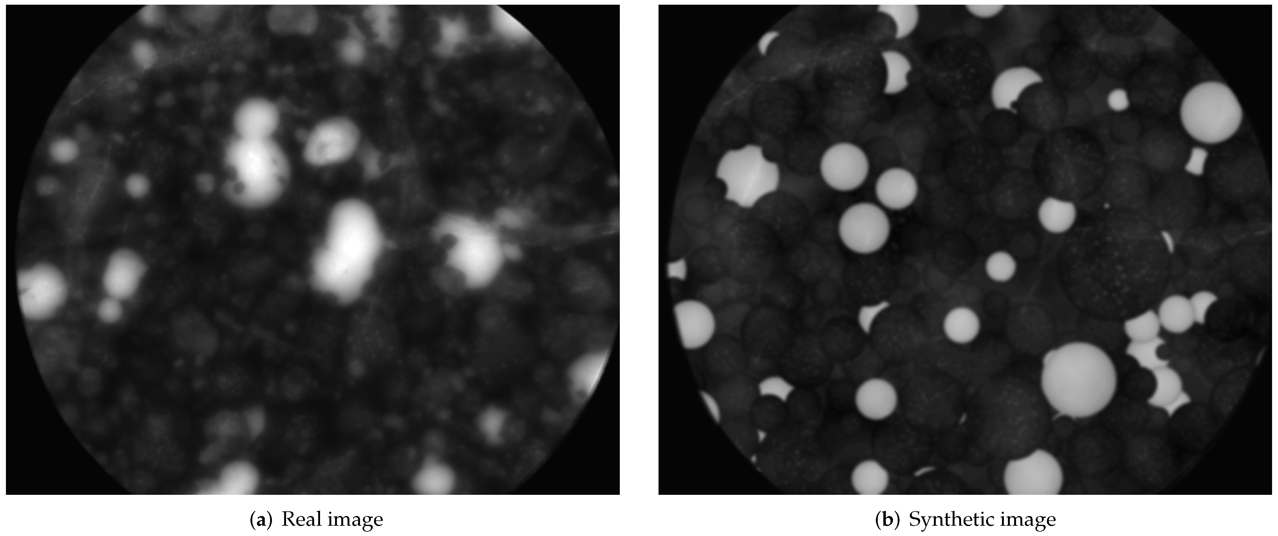
While training data are directly used for the training—i.e., the optimization of the weights—of the utilized neural networks, validation data are only used to evaluate the performance of said networks during the training. It was therefore at most an indirect influence on the network weights, e.g., by stopping the training as soon as the validation performance ceases to improve (early stopping, see also Section 3.1.1). For the studies at hand, the training and validation data sets consisted of 400 synthetic images (featuring 107,930 dark and 13,314 light particles) and 20 synthetic images (featuring 5353 dark and 648 light particles), respectively. Increasing the number of synthetic training images to 800 did not yield any significant improvement. For details concerning the PSD properties of the synthetic training and validation images, please refer to Section 3.1.2.

2.2. Test Data

The test data are never used during training (not even indirectly) but solely to judge the performance of the proposed method and compare it to that of the fully-automated benchmark method (see Section 3.2.2). For the publication at hand, the test data consisted of a set of 12 real images, accompanied by the results of a trifold manual annotation, i.e., carried out by three independent operators (see Figure 2a–c, Section 3.2.1).

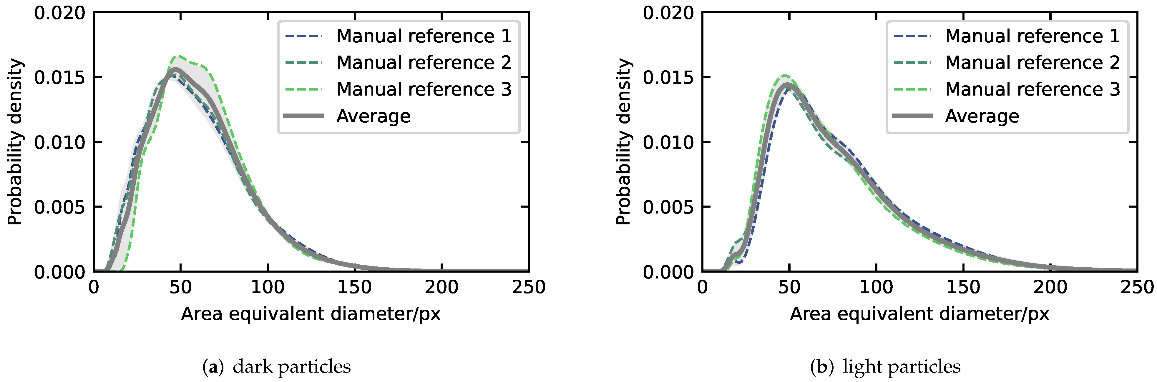
2.2.1. Average Particle Size Distribution

Since even the manual annotation is not perfect, the results from the three different operators vary slightly. Figure 3 and

Table 1. Particle size distribution properties (geometric mean diameter d_g, geometric standard deviation σ_g, and number of particles N) of dark and light populations of three manual references and averaged manual reference (mean ± standard deviation of d_g and σ_g, respectively).

	Dark Particles			Light Particles
	dg	σg	N	dg	σg	N
Manual reference 1	$54.0$ px	1.63	1525	$72.0$ px	1.54	325
Manual reference 2	$53.0$ px	1.64	1106	$68.5$ px	1.61	335
Manual reference 3	$58.7$ px	1.48	864	$65.7$ px	1.55	328
Manual reference (avg.)	$55.2\pm 2.5$ px	1.58 ± 0.08	–	$68.7\pm 2.6$ px	1.57 ± 0.03	–

show comparisons of the resulting PSDs. Light particles (Figure 3b) are easier to annotate for human operators than dark particles (Figure 3a). Since dark particles are much more frequent and also smaller, they have a high chance of being surrounded by other dark particles, which makes them difficult to locate, due to the low contrast. Conversely, light particles tend to be larger and less frequent, so that they are more often surrounded by dark particles than other light particles, which results in a higher contrast and therefore an easier annotation process.

To compensate for the uncertainty that is introduced by the manual annotation, the manual reference PSDs for both dark and light particles were averaged to form the PSDs, used as benchmarks for the tested particle mixture analysis methods (see Figure 3 and Table 1). The averaging was carried out as follows for each of the involved particle classes (dark and light):

• Fitting of the raw data of each of the manual references via Gaussian kernel density estimations (KDEs) in the log-normal space, using Scott’s Rule [16] to select a suitable bandwidth for the estimation. For an elaboration upon this method, please refer to Scott [16].
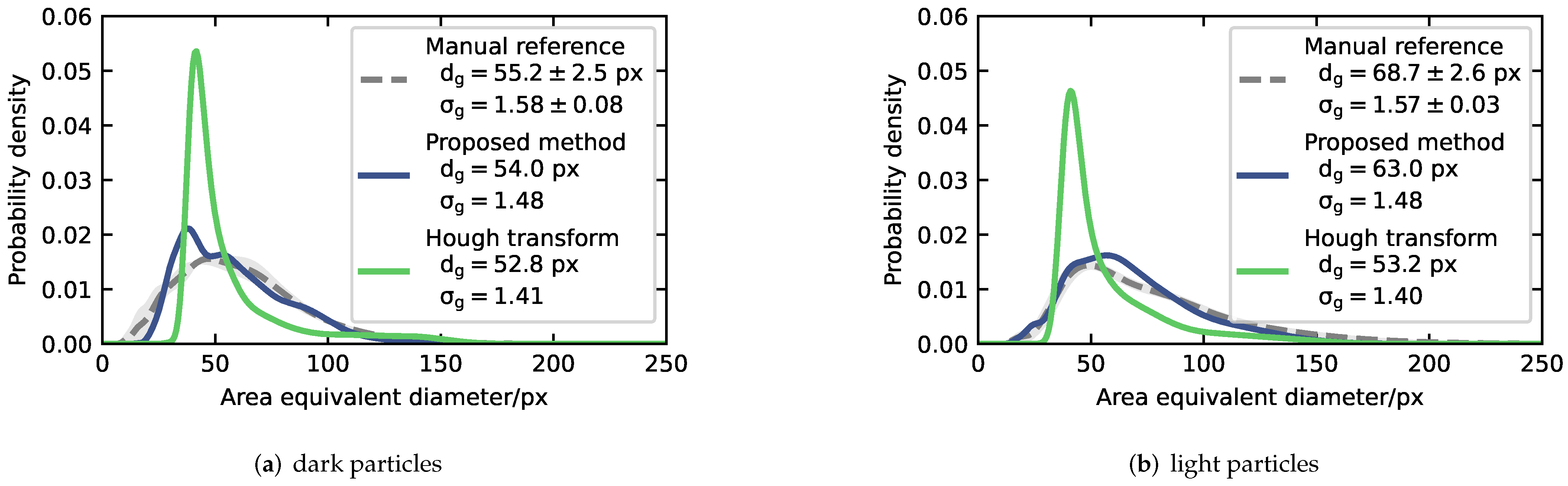
• Interpolation of the three resulting KDEs at 200 linearly spaced support values, between the minimum and maximum observed area equivalent diameters (see Figure 3a,b, dashed lines).
• Averaging of the probability densities acquired by the interpolation, to yield means (see Figure 3a,b, solid lines) and standard deviations (see Figure 3a,b, shaded areas) for each of the support values.
• Calculation of the means and standard deviations of the characteristic properties (geometric mean diameter d_g and geometric standard deviation σ_g) of the reference PSDs (see Table 1).

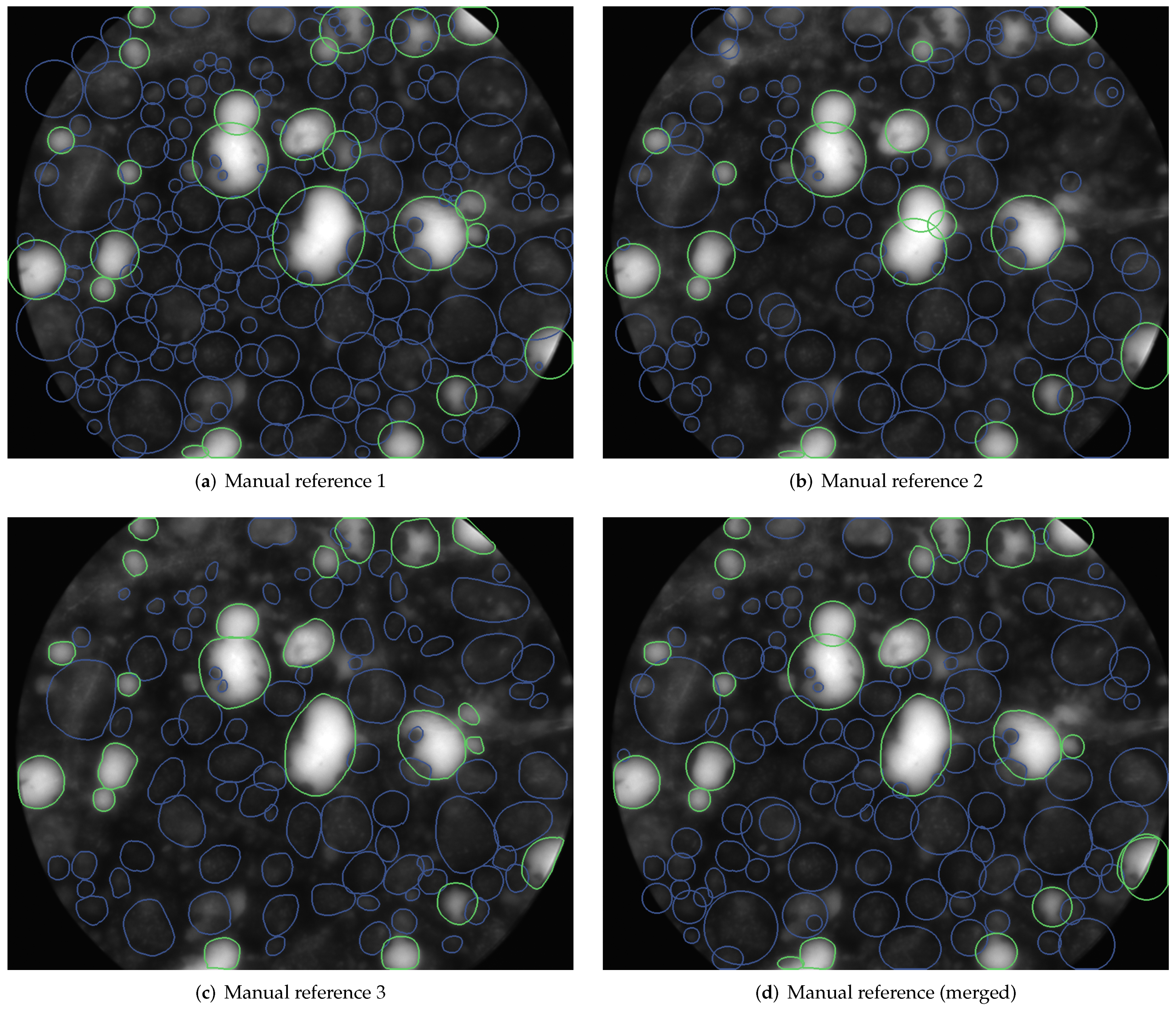
2.2.2. Merged Annotations

While the evaluation of the PSD measurement quality of a given method is ensemble-based, the evaluation of the object detection quality is instance-based. In computer vision, an instance refers to an object of a certain class, e.g., a particle. This means that missing or redundant particles affect the latter significantly more than the former. To attain an object detection reference as complete as possible, the three manual references were merged into a single reference. The merging was carried out based on a voting system, where only instances that are present in at least two of the three manual reference annotations (see Figure 2a–c) were carried over to the merged annotation (see Figure 2d). Identical instances in the three manual annotations were identified based on their intersection over union (IoU), using an IoU threshold of 50%, which was chosen in line with the matching criterion used by the prominent Pascal VOC [17] and COCO [18] object detection challenges. From the sets of identical instances resulting from the voting process, only a single instance per set was chosen randomly for the merged annotation to avoid duplicates.

Intersection over Union

The intersection over union (IoU, also referred to as Jaccard or Tanimoto index) is a common metric for object detection tasks. It is used to measure the similarity of two objects, taking into account not only their shape and size, but also their position (see Figure 4). It can therefore be used to compare a prediction of an algorithm to the so-called ground truth, which in machine learning, refers to the best available data to test a prediction of an algorithm (i.e. the ground truth is not necessarily perfect itself).

As the name implies, it is defined as the ratio of the area of intersection and the area of the union of two objects A and B:

$$\mathrm{IoU}(A,B)=\frac{|A\cap B|}{|A\cup B|}$$

(1)

3. Methods

Apart from the proposed method itself (see Section 3.1) this section also elaborates upon the methods used to benchmark its performance (see Section 3.2).

3.1. Proposed Method

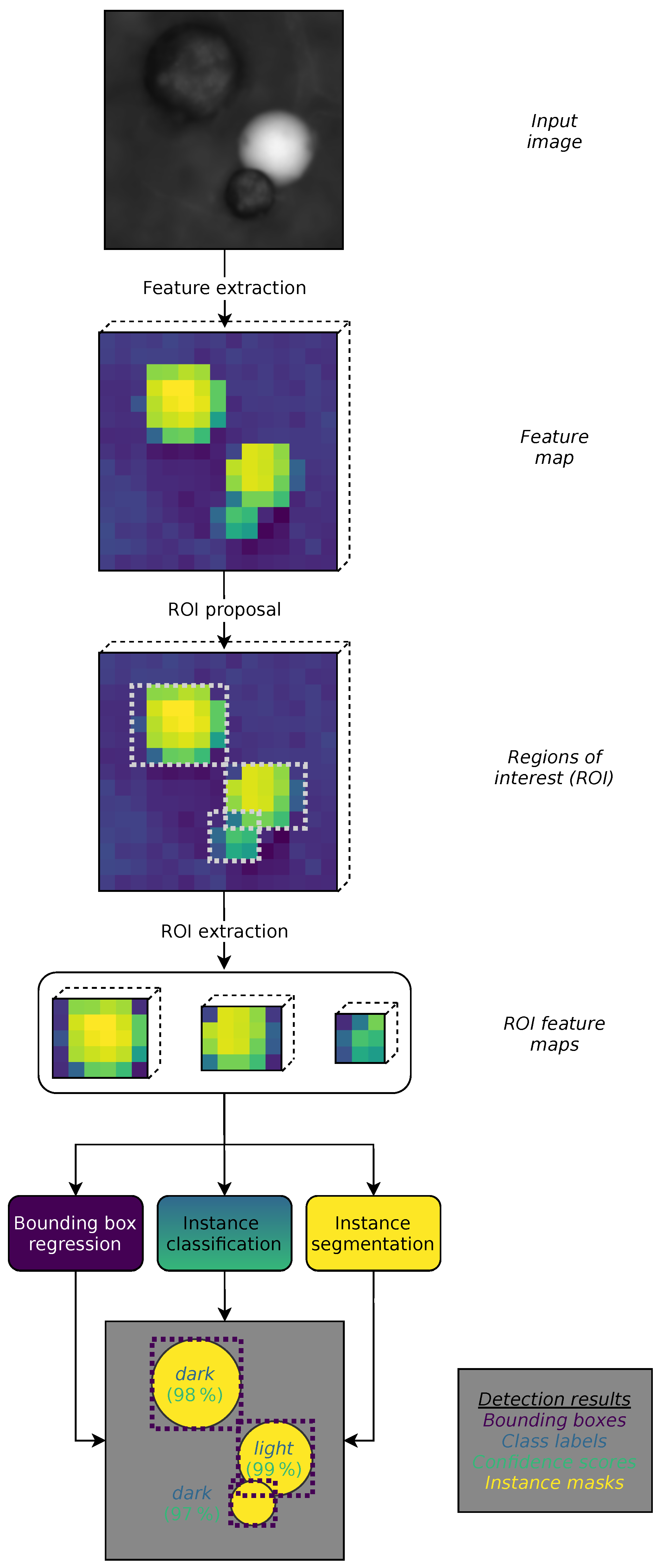
The proposed method consists of two parts: Mask R-CNN (see Section 3.1.1) and image synthesis (see Section 3.1.2).

Mask R-CNN [13], is a well-established region-based convolutional neural network (R-CNN) architecture for object detection. As such, it requires large amounts of already annotated images, to be used for its supervised training process. To avoid the laborious creation of the training data via manual annotation, we propose the use of image synthesis.

3.1.1. Mask R-CNN

The following section will give a brief overview of the working principles of the Mask R-CNN architecture, which consists of six stages (see Figure 5; For a more detailed explanation, please refer to He et al. [13].): feature extraction, region of interest (ROI) proposal/extraction, bounding box regression, instance classification and instance segmentation.

During the feature extraction, the input image is fed to a large CNN (the backbone) to extract the so-called feature map using image convolution (hence the name CNN). The utilized convolution kernels are learned during the training, based on the supplied training data. The feature extraction is a step-wise process. With each step, the lateral resolution of the image is reduced in return for progressively more semantic, i.e., meaningful in the context of the given task, information about each remaining pixel. As a result, the feature map has not just two but three dimensions, where the third dimension holds semantic information about each pixel, just as the third dimension of an RGB image holds semantic information about the redness, greenness, and blueness of its pixels.

For the ROI proposal/extraction, a fixed number of potential ROIs is generated, without taking the feature map into consideration. Then, a small neural network is used to predict the objectness score of each potential ROI based on its content. Subsequently, ROIs with a low score or a high overlap with higher-score ROIs are discarded, while the remaining ROIs are extracted, by simply cutting them out of the feature map. The result is a set of instance feature maps, i.e., one feature map for each object in the input image. Ultimately, the set of instance feature maps is resized to a uniform size using ROI alignment and passed to each of the downstream network branches. The details of ROI alignment are beyond the scope of this publication. For an in-depth explanation, please refer to He et al. [13].

The goal of the bounding box regression (regression: prediction of continuous values) is to predict the coordinates and dimensions of the bounding boxes of the objects in the ROIs, by means of a small fully-connected neural network. This step is necessary, since the ROIs themselves correspond to the feature map, which has a very low spatial resolution, rather than the high-resolution input image.

During the instance classification (classification: prediction of discrete values), a class label for each of the objects in the ROIs is predicted by another small fully-connected neural network, along with a confidence score. This step is crucial for the analysis of particle mixtures. For the images used withing this publication, there are two classes: dark and light particles.

The instance segmentation uses a small CNN, to upsample the low-resolution, high-depth feature map associated with each ROI to a high-resolution, low-depth binary mask, conversely to the downsampling carried out by the backbone during the feature extraction. The resulting mask has the same size as the bounding box and each of its pixels is either true, if the corresponding pixel of the ROI belongs to the object, or false if not.

Implementation Details

The implementation of Mask R-CNN used for this publication is available as part of the self-implemented paddle (PArticle Detection via Deep LEarning; https://github.com/maxfrei750/paddle; accessed date: 1 December 2021) toolbox, which makes use of Python and the following mentionable packages: (i) PyTorch [19], Torchvision [19] and PyTorch Lightning [20] for the construction and training of neural networks; (ii) Albumentations [21] for image augmentation, which is an easy way to artificially increase the size of a training data set by applying transformations to the input images (for the studies at hand, vertical and horizontal flipping was applied to the training data, each with a probability of 50%); (iii) Hydra [22] for the comfortable handling of configuration files as well as (iv) Weights & Biases [23] and Tensorboard [24] for experiment logging.

One of the great advantages of Mask R-CNN is that the backbone is easily interchangeable to meet the needs of different applications. For this publication, the convolutional blocks of the ResNet-50 network [25] were used as backbone. For an elaboration upon the reasoning behind this design choice, please refer to Frei & Kruis [10]. Also, the maximum number of detections per image was increased to 400, based on the maximum number of instances in the synthetic training images (see Section 3.1.2).

Apart from the network architecture, the strategies used during the training process are fundamental to its success. For the publication at hand, the main goal (apart from a good performance) of the training strategies was to avoid the need for time-consuming optimization of hyperparameters (i.e., parameters of the utilized learning algorithm that have to be specified manually and are not optimized by the learning algorithm itself, e.g., learning rate, training duration, etc.). This was achieved with a combination of two techniques: early stopping and learning rate scheduling. Both of these techniques are based on the monitoring of a validation metric, to measure the performance of the neural network in training, on a set of validation data. Early stopping automatically determines a suitable training duration, by stopping the training as soon as the validation metric does not improve over a certain amount of training epochs (20). Similarly, the utilized learning rate scheduling automatically determines the optimum learning rate—which is the most important hyperparameter [26]—by dropping the base learning rate (0.005) by a predefined factor (10) if the validation metric does not improve over a certain amount of training epochs (10). As validation metric, the mean average precision on the set of validation images is being used. For a comprehensive elaboration upon this metric, please refer to Frei & Kruis [11].

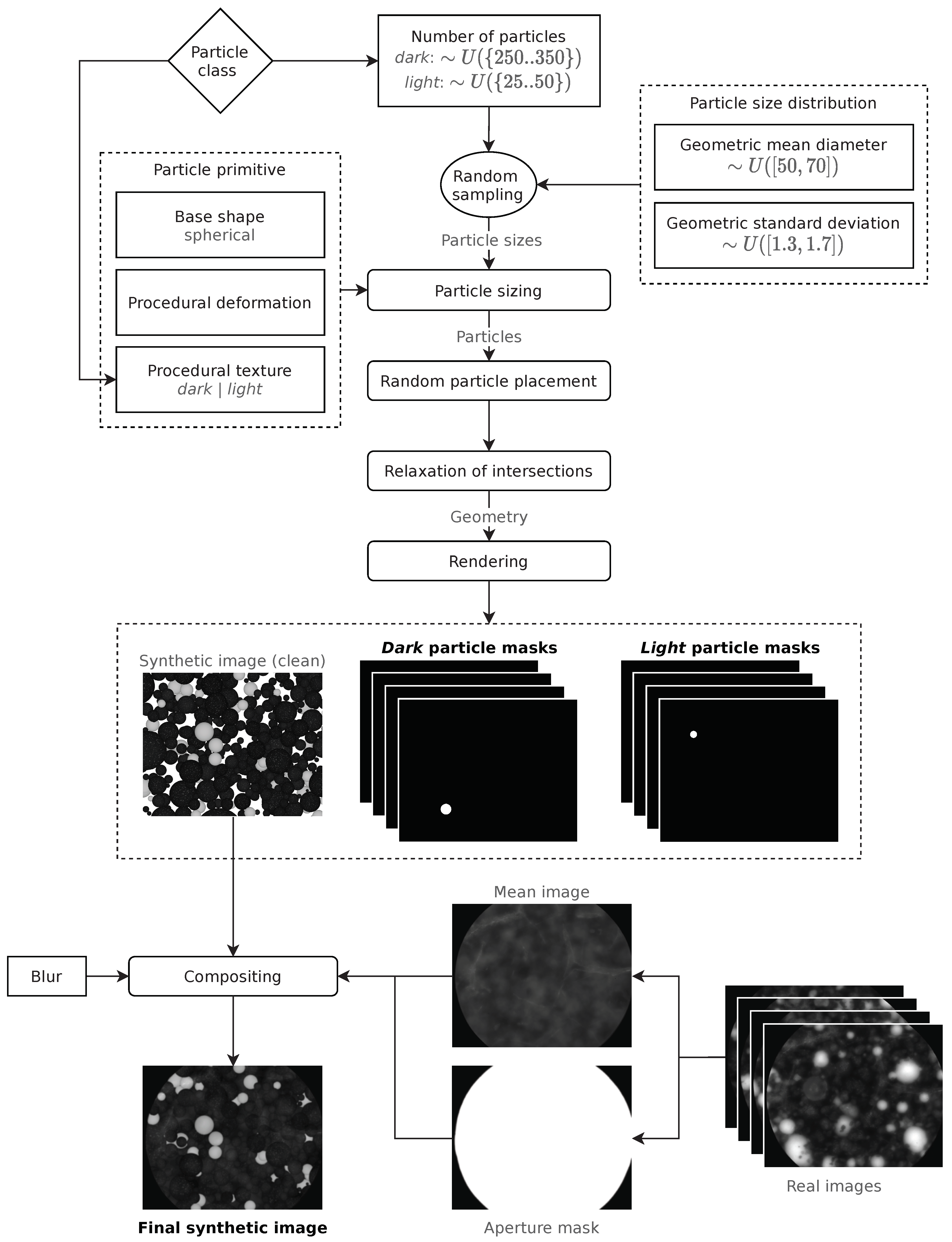
3.1.2. Image Synthesis

The synthetic data, used for the training and validation of the utilized Mask R-CNN, were created using the self-implemented synthPIC (SYNTHetic Particle Image Creator; https://github.com/maxfrei750/synthPIC4Python; accessed date: 1 December 2021) toolbox, which is based on Blender [27] controlled by Python [28]. While synthPIC offers a wide variety of tools to synthesize life-like particle images, only the features used for the publication at hand shall briefly be elaborated upon.

Figure 6 illustrates the image synthesis procedure of a single synthetic image. The first fundamental step of the image synthesis is the creation of geometry. Since the real data feature a mixture of dark and light particles, the geometry creation is based on two particle populations as well. Each population, in each image, consists of three components:

• A unique random PSD, represented by a geometric mean diameter d_g (in pixels) and a geometric standard deviation σ_g, both picked from a wide uniform distribution U of plausible values:

  $$\begin{array}{c}{d}_{\mathrm{g}}\sim U\left(\right[50,70\left]\right)\end{array}$$

  (2)

  $$\begin{array}{c}{\sigma }_{\mathrm{g}}\sim U\left(\right[1.3 ,1.7\left]\right)\end{array}$$

  (3)
• A number of particles N, which is picked from a uniform distribution U, with different boundaries for dark and light particles, since in the real images, there are many more dark than light particles:

  $$\begin{array}{c}{N}_{\mathrm{dark}}\sim U\left(\{250..350\}\right)\end{array}$$

  (4)

  $$\begin{array}{c}{N}_{\mathrm{light}}\sim U\left(\{25..50\}\right)\end{array}$$

  (5)
  The boundaries were chosen based on the resulting similarity of the synthetic images to the real images used for the testing of the proposed method.
• A so-called particle primitive, which serves as prototype for the particles of the respective population. Each primitive features a certain base shape, a procedural (i.e., based on randomizable parameters) deformation and a procedural texture (this is where dark and light particles differ).

After all particles for an image were created by duplicating the particle primitives and resizing them according to the respective PSD, the particles are placed in the 3D simulation space. The particles are placed randomly, however within the boundaries of the 2D projection that is ultimately required to calculate the image. Due to the high number of particles, the placement can result in intersecting particles. To relax these intersections, and to create a dense particle ensemble that resembles the real images, synthPIC uses the built-in rigid body physics simulation of Blender, which pushes objects apart, proportionally to their overlap, until they no longer intersect.

The second fundamental step of the image synthesis process is the rendering, which makes use of Blenders built-in rendering engines, to produce a clean version (i.e., without distortions) of the synthetic image and the corresponding particle masks. While it is possible with synthPIC, the masks do not account for occlusions, since initial experiments showed that this deteriorated the performance of the proposed method.

The third and last fundamental step of the image synthesis is the compositing, which takes the clean image and makes it more lifelike by adding distortions (e.g., blur) and characteristic image features such as the very prominent aperture mask and the lens texture, which are identical for each of the real images. While the former was extracted using a graphics editor (GIMP [29]), the latter was attained by averaging the available real images to extract the mean image.

The parameters of the image synthesis were chosen to subjectively match the style and appearance of the real test data. Figure 1 depicts a comparison of a synthetic and a real example image.

3.2. Benchmark Methods

There are two kinds of benchmarks for the proposed method: on the one hand, it needs to be compared to the most accurate method for image-based particle mixture analysis currently available, i.e., manual annotation, to test its accuracy. On the other hand, it makes sense to compare the proposed method to another fully automated method for the image-based analysis of particle mixtures to asses how it contributes to the goal of reliable full automation.

3.2.1. Manual Analysis

While manual annotation is still the gold standard of image-based particle analysis when it comes to accuracy, it is far from perfect. Especially for ambiguous images, e.g., due to a low contrast and blur, annotation results can vary dramatically (see Figure 2). For the images at hand, this is especially problematic for the dark particle class. To alleviate this problem, the images used for the testing of the proposed method were analyzed not only once, but a total of three times by two in-house operators and one external operator (see also Section 2.2). While the two in-house operators used identical methods, the external analysis was carried out with the default methods of the external party to achieve a truly independent analysis.

Prior to the annotation, each image was preprocessed using the Image-Pro Plus software [30], to enhance the image clarity and contrast (see Figure 7). The preprocessing consisted of two steps: (i) A gamma correction with a factor of 1.7 and (ii) the application of the HiGauss filter [31] with a size of $9\times 9$ and a strength of 10.

Manual references 1 and 2 (see Figure 2a,b) were created in-house using the popular ImageJ software [32]. Each image was annotated in two separate passes, one for the dark particles and one for the light particles, using the elliptical selection tool. Consequently, the resulting annotations are all strictly elliptical or even circular. Manual reference 3 (see Figure 2c) was also created in two separate passes but by an external service specialized in imaging-particle analysis, using an annotation tool based on free-hand drawing. Annotations can therefore have arbitrary shapes.

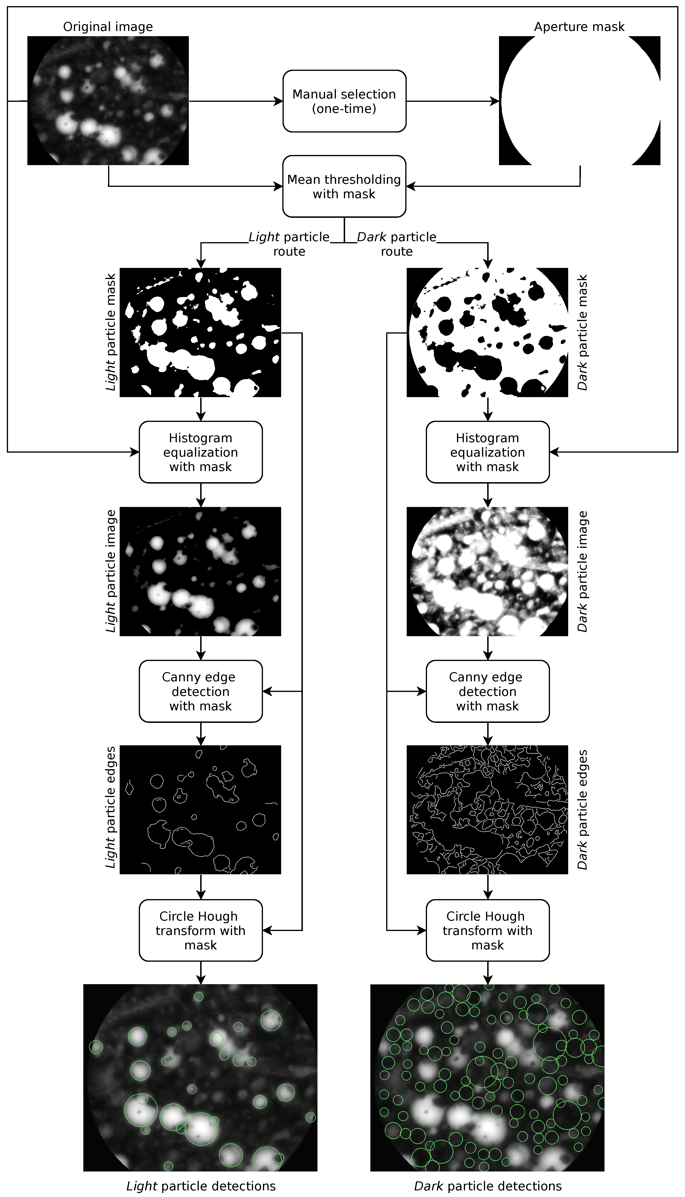
3.2.2. Hough Transform

As an example of a conventional, i.e., not machine learning-based, fully automated method for the image-based analysis of particle mixtures, a workflow based on mean thresholding, histogram equalization [33,34], Canny edge detection [35], and the Hough transform (HT) [36] was implemented using Python [28] with the skimage package [37], to be used as a benchmark for the proposed method.

The principal steps of the conventional workflow (see Figure 8) are as follows.

Aperture Mask Extraction

The utilized images all feature an identical aperture mask. Since the dark regions of this mask do not hold any meaningful information, it is sensible to exclude them from the image analysis. The extraction of the aperture mask was carried out manually, using a graphics editor (GIMP [29]).

Mean Thresholding with Mask

To discriminate light and dark particles, the original image is binarized using mean thresholding, resulting in a light particle mask, where true pixels represent pixels belonging to light particles and a dark particle mask, where true pixels represent pixels belonging to dark particles. For the creation of the light particle mask, pixels with an intensity larger than the mean intensity value of the original image pixels were set to true. Complementary, for the creation of the dark particle mask, pixels with an intensity smaller or equal to the mean intensity value of the original image pixels were set to true. In both cases, pixels corresponding to false pixels in the aperture mask were not considered during the calculation of the mean pixel intensity and were set to false themselves. From this point on-wards, the workflow splits into a light and a dark particle route, both of which operate identically but on different parts of the original image.

Since the utilized automated binarization method plays a crucial role for the performance of the conventional fully-automated benchmark method, its choice shall be briefly elaborated upon.

Figure 9 depicts a comparison of the histograms of the pixel intensities of the images of the test data set. Evidently, (i) all images feature quasi-identical histograms; and (ii) there is just a single mode, i.e., the differentiation of dark and light particles based on the pixel intensity is a challenging task.

To find an optimal automated binarization method, six different methods were tested: the iterative self-organizing data analysis technique (ISODATA) [38], Li’s minimum cross entropy method [39], mean thresholding, the minimum method [40], Otsu’s method [41] and the triangle method [42]. Each of the methods was applied to the images of the test set and the resulting thresholds were plotted in form of a box plot (see Figure 10). Based on the results, the minimum method and the triangle method were disqualified, since they yield abnormally high, respectively low thresholds and therefore unusable binarization results. While the remaining methods generally produce similar thresholds, only the mean thresholding method does not produce implausible outliers—since all test images feature quasi-identical histograms (see Figure 9), they should also result in quasi-identical thresholds—and was therefore used for the conventional fully-automated benchmark method.

Histogram Equalization with Mask

Since the contrast of the original images is low, especially in the region of the dark particles, histogram equalization [33,34] is applied in the areas covered by the light and dark particle masks, respectively.

Canny Edge Detection with Mask

The contrast enhanced dark and light particle images are processed using Canny edge detection [35], so that only the edges of the respective particle class are extracted. Edges outside of the corresponding particle mask are being ignored.

Circle Hough Transform with Mask

The dark and light particle edges resulting from the previous processing step are used to carry out two separate circle Hough transforms [36], one for each particle class. To improve the detection results for the respective particle class, circles that are primarily outside of the corresponding particle mask are being removed.

4. Results

In this section, various aspects of the performance of the proposed method with respect to both detection quality (see Section 4.1) and PSD analysis (see Section 4.2) will be evaluated, by comparing its results to those of a manual analysis, as well as those of a conventional fully automated method, based on the HT. For details concerning these benchmark methods, please refer to Section 3.2.

The source code and model, as well as training, validation and test data, used for the training of the proposed method and the generation of the results presented in this section are available via the following link: https://github.com/maxfrei750/ParticleMixtureAnalysis/releases/v1.0 (accessed date: 1 December 2021).

4.1. Detection Quality

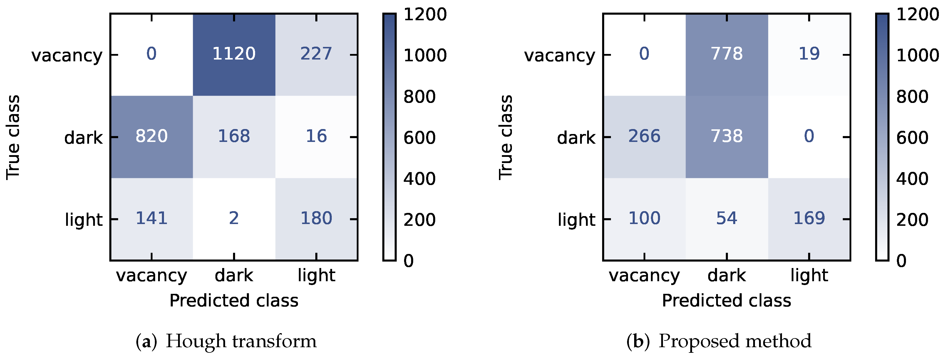
Since the assessment of the detection quality is instance-based, the merged manual reference (see Section 2.2.2) will be used as basis for the evaluation throughout this section. To get a first, qualitative impression of the detection quality of the proposed method, Figure 11 compares a random selection of example detections to the merged manual reference, as well as the results of the HT.

Both the proposed method and the HT tend to overlook or misclassify some of the particles (regardless of their class). Subjectively, the clustered detections of the proposed method resemble the manual reference much closer than the more spread out, random-looking detections of the HT. Interestingly, the proposed method sometimes produces ambiguous classifications, where light particles are classified as light as well as dark.

Classification

For object detection tasks, the evaluation of the classification capabilities of a method is more complicated than for more basic tasks, such as image classification, since it requires a positional matching of predictions and targets of each image.

For the studies at hand, the matching was carried out as follows: The predictions are iterated in descending order of their confidence scores (see Section 3.1.1; for the HT, all confidence scores are 100%). Each prediction is matched with the ground truth instance that results in the highest IoU (see Section 2.2.2) and was not used in a previous match, but only if $\mathrm{IoU}\ge 50\%$.

Additionally to the two original classes dark and light, this matching process introduces a third class: the vacancy class. For example, a prediction without a matching ground truth instance should have had the class vacancy. Likewise, if there is no matching prediction for a given ground truth instance, the tested method passively made an incorrect virtual prediction of class vacancy. For the HT, this is the only way to make a vacancy prediction. In contrast, the proposed method can correctly predict the vacancy class via the confidence score (see Section 3.1.1) that comes with every predicted instance. If the confidence score is below 50% (regardless of the originally predicted label), then the corresponding instance can considered to belong to the vacancy class. However, this might give an unfair advantage to the proposed method during the calculation of classification accuracies (see Equations (6) and (7) and

Table 2. Comparison of proposed method and Hough transform, with respect to their overall accuracy ACC, object vs. vacancy accuracy ACC_obj.|vac. and dark vs. light accuracy ACC_dark|light.

	Hough Transform	Proposed Method
accuracy	$13.0$%	$42.7$%
ACCobj.|vac.	$13.7$%	$45.2$%
ACCdark|light	$95.1$%	$94.4$%

), if it produced a lot of correct vacancy predictions. Therefore, to level the playing field, predictions of the proposed method with a confidence score below 50% were discarded, thereby artificially robbing it of the ability to make correct predictions of class vacancy.

For a classification with three classes, there are nine possible outcomes for each instance, which can be ordered in a so-called confusion matrix, which compares the predicted class of an instance with the true class it was supposed to have. Figure 12 compares the confusion matrices of the HT and the proposed method. The proposed method outperforms the HT for the vacancy and dark classes by a large margin, while the latter performs slightly better for the light particle class.

The overall accuracy $\mathrm{ACC}$ of a method can be calculated based on the true predictions $T_{\mathrm{t}}=X_{\mathrm{tp},[\mathrm{t}=\mathrm{p}]}$ and the false predictions $F_{\mathrm{tp}}=X_{\mathrm{tp},[\mathrm{t}\ne \mathrm{p}]}$

$$\mathrm{ACC}=\frac{{\sum }_{\mathrm{t}}{T}_{\mathrm{t}}}{{\sum }_{\mathrm{t}}{T}_{\mathrm{t}}+{\sum }_{\mathrm{t},\mathrm{p}}{F}_{\mathrm{tp}}}=\frac{{\sum }_{\mathrm{t}}{T}_{\mathrm{t}}}{{\sum }_{\mathrm{t},\mathrm{p}}{F}_{\mathrm{tp}}},$$

(6)

where X_tp prediction is a prediction, while t and p are the true and predicted classes, respectively. This means that the accuracy is equal to the number of correct predictions divided by the total number of predictions.

Conceptually, the overall accuracy of a method for the given classification task is a result of its capabilities to differentiate between (i) an object and a vacancy and (ii) dark and light particles. It is therefore possible to attain more detailed insights concerning the object vs. vacancy accuracy ACC_obj.|vac. by joining the dark and light classes into a combined object class:

$${\mathrm{ACC}}_{\mathit{obj}.|\mathit{vac}.}=\frac{{\sum }_{\mathrm{t}}{T}_{\mathrm{t}}+F_{\mathit{light},\mathit{dark}}+F_{dark,light}}{{\sum }_{\mathrm{t},\mathrm{p}}{X}_{\mathrm{tp}}}$$

(7)

Contrarily, it is possible to study the dark vs. light accuracy ACC_dark|light by dropping the vacancy class:

$${\mathrm{ACC}}_{\mathit{dark}|\mathit{light}}=\frac{T_{dark}+T_{light}}{T_{dark}+T_{light}+F_{dark}+F_{light}}$$

(8)

Table 2 compares the proposed method and the Hough transform, with respect to their overall accuracy ACC, object vs. vacancy accuracy ACC_obj.|vac. and dark vs. light accuracy ACC_dark|light.

Both methods succeed at discriminating dark and light particles, provided that particles as such are identified successfully. However, the proposed method significantly outperforms the HT with respect to the overall accuracy, since it features a much higher accuracy with respect to the differentiation of objects and vacancies. The reason for its better object detection capabilities is presumably the inherently more adaptive nature of the proposed method, with respect to the initial feature extraction. While the HT relies on rather static methods (see Section 3.2.2), whose parameters need to be tweaked manually and can therefore never be optimal, the proposed method automatically custom-tailors the feature extraction to the input data during the training process.

Still, the accuracy of the proposed method leaves room for future improvements. Potential approaches are (i) improvements of the image synthesis to achieve more lifelike training data, e.g., using image similarity metrics; and (i) supplementation of the synthetic training data with real training data, attained by manually correcting erroneous detections in the outputs of the proposed method in its current state.

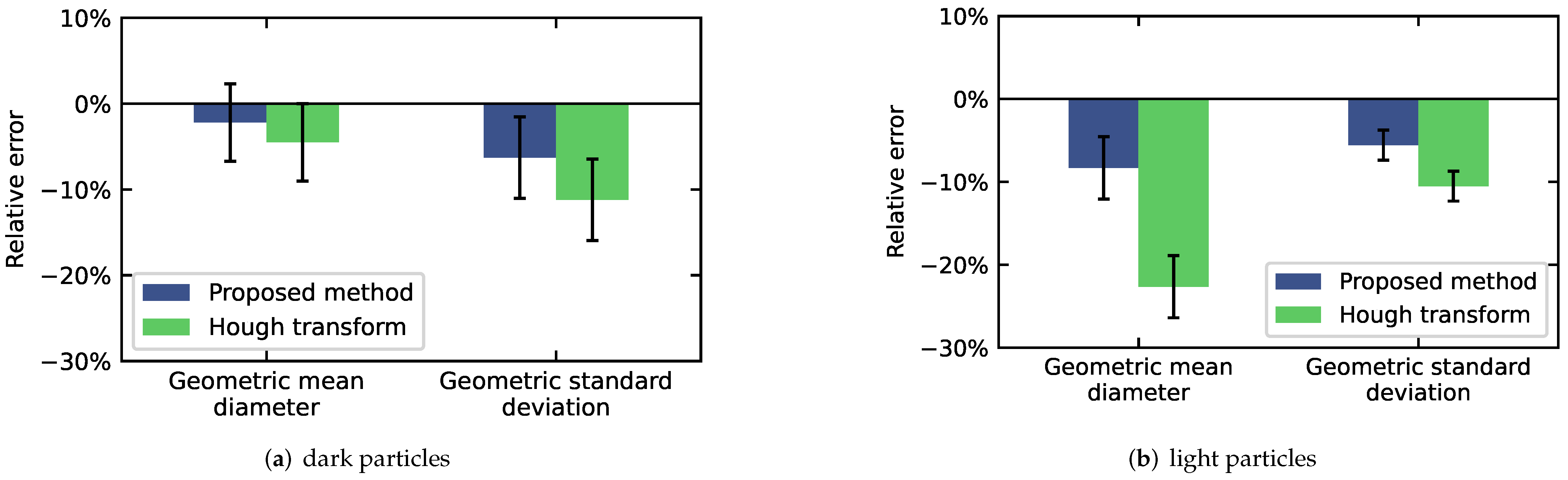
4.2. Particle Size Distribution Analysis

The end use of the proposed method is the analysis of the PSDs of the different fractions of a particle mixture, which is the direct result of its capabilities to identify and label, as well as classify individual particles.

To calculate the PSD from a set of detection results for a certain class, the area equivalent diameter of the resulting detection masks was calculated and a Gaussian KDE [16] was carried out in the log-normal space, using Scott’s Rule [16] to select a suitable bandwidth for the estimation. For the proposed method, each observation was weighted according to its confidence score.

Figure 13 compares the PSDs that were obtained using the proposed method and the HT with the manual reference annotations, for both dark and light particles. The proposed method clearly outperforms the HT, for both classes and provides PSDs that resemble the manual references more closely. The HT produces quasi-identical PSDs for the dark and light particle fractions, while the proposed method is better at picking up the subtle differences in the two particle ensembles that are apparent in the manual references. Nevertheless, the proposed method still leaves room for improvements. Particularly striking in this respect are the implausible peaks of the PSDs that the proposed method produces at area equivalent diameters of $d_{\mathrm{A}}\approx 38\mathrm{px}$ and $d_{\mathrm{A}}\approx 54\mathrm{px}$ (for dark particles), as well as $d_{\mathrm{A}}\approx 24\mathrm{px}$ and $d_{\mathrm{A}}\approx 60\mathrm{px}$ (for light particles). The examination of the exact reasons for these artifacts is beyond the scope of this publication and will therefore be subject to future investigations. However, it can be hypothesized that they are the consequence of aliasing effects, resulting from discretizations within the architecture of the utilized CNN. Potential candidates for such effects are the downsampling mechanisms (convolution and pooling) in the backbone (see Section 3.1.1), as well as the utilization of discrete bounding box sizes (among them 32 px and 64 px) during the ROI proposal. Potential remedies could be the use of alternative backbone architectures (e.g., transformer-based, i.e., non-convolutional), or finer step sizes during the ROI proposal.

To quantify the previous qualitative assessments of the PSD analysis, the geometric mean diameter and geometric standard deviation of the measured PSDs were calculated for the proposed method and the HT, for both classes (see Figure 13, legends). Subsequently, the errors of the PSD properties of the tested methods were calculated, relative to the average PSD properties of the manual references (see Section 2.2.1). Figure 14 depicts a comparison of these relative errors. Overall, the proposed method features smaller relative errors, which are even in the range of the uncertainty of the manual reference for the dark particle class. Unlike human operators, both automated methods fare worse for light particles than for dark particles. While these differences are within the range of uncertainty for the proposed method, they are significant for the HT. Ergo, the proposed method not only excels with respect to accuracy, but also interclass consistency, which may be of special interest, depending on the application of the surveyed particle mixture.

5. Conclusions

This work made a progress toward the fully automated image-based analysis of dense particle mixtures using Mask R-CNN, a prominent deep learning-based object detection architecture, and image synthesis.

The proposed method was tested on a set of endoscopic images of particle mixtures stemming from an FCC plant, and its results were compared to those of a conventional benchmark method for the image-based analysis of particle mixtures based on the HT, as well as a trifold manual analysis. While the benchmark method achieved only a low detection/classification accuracy ($13.0$%) compared to that of the proposed method ($42.7$%), the latter still leaves room for improvement. On the one hand, the lifelikeness of the synthetic training images still leaves much to be desired and can presumably be drastically improved by the use of advanced generative methods, such as generative adversarial networks (GANs). On the other hand, the feature extraction of the utilized Mask R-CNN can be updated to use a more powerful architecture, e.g., replacing the utilized CNN by a transformer network. Results from other fields of computer vision (e.g., classification) give reason for hope that, in the long-term, a human or even super-human performance might be feasible.

Nevertheless, even today, the proposed method already provides a usable precision with respect to the measurement of mixture component PSDs, featuring errors (relative to the manual reference) as low as $\Delta d_{\mathrm{g}}=-2\pm 5\%$ and $\Delta {\sigma }_{\mathrm{g}}=-6\pm 5\%$ for the dark particle class, as well as $\Delta d_{\mathrm{g}}=-8\pm 4\%$ and $\Delta {\sigma }_{\mathrm{g}}=-6\pm 2\%$ for the light particle class.

It thereby significantly outperforms the HT-based benchmark method, which features errors of $\Delta d_{\mathrm{g}}=-5\pm 5\%$ and $\Delta {\sigma }_{\mathrm{g}}=-11\pm 5\%$ for the dark particle class, as well as $\Delta d_{\mathrm{g}}=-23\pm 4\%$ and $\Delta {\sigma }_{\mathrm{g}}=-11\pm 2\%$ for the light particle class.

Remarkably, for the dark particle class, which is notoriously difficult to annotate even for humans, the relative errors of the proposed method are already comparable to or even smaller than the uncertainty of the human reference measurements.

All in all, the proposed method is a viable method for the image-based analysis of dense particle mixtures.

References

1. Schulze, D. Pulver und Schüttgüter: Fließeigenschaften und Handhabung, 3., erg. Aufl. 2014 ed.; VDI-Buch, Springer: Berlin/Heidelberg, Germany, 2014. [Google Scholar]
2. Kaye, B.H. Powder Mixing, 1st ed.; Powder Technology Series; Chapman & Hall: London, UK, 1997. [Google Scholar]
3. Sadeghbeigi, R. Fluid Catalytic Cracking Handbook: Design, Operation, and Troubleshooting of FCC Facilities, 2nd ed.; Gulf: Houston, TX, USA, 2000. [Google Scholar]
4. Musha, H.; Chandratilleke, G.R.; Chan, S.L.I.; Bridgwater, J.; Yu, A.B. Effects of Size and Density Differences on Mixing of Binary Mixtures of Particles. In Powders & Grains 2013, Proceedings of the 7th International Conference on Micromechanics of Granular Media, Sydney, Australia, 8–12 July 2013; AIP Publishing LLC: Melville, NY, USA, 2013; pp. 739–742. [Google Scholar] [CrossRef]
5. Shenoy, P.; Viau, M.; Tammel, K.; Innings, F.; Fitzpatrick, J.; Ahrné, L. Effect of Powder Densities, Particle Size and Shape on Mixture Quality of Binary Food Powder Mixtures. Powder Technol. 2015, 272, 165–172. [Google Scholar] [CrossRef]
6. Daumann, B.; Nirschl, H. Assessment of the Mixing Efficiency of Solid Mixtures by Means of Image Analysis. Powder Technol. 2008, 182, 415–423. [Google Scholar] [CrossRef] [Green Version]
7. Zuki, S.A.M.; Rahman, N.A.; Yassin, I.M. Particle Mixing Analysis Using Digital Image Processing Technique. J. Appl. Sci. 2014, 14, 1391–1396. [Google Scholar] [CrossRef]
8. Realpe, A.; Velázquez, C. Image Processing and Analysis for Determination of Concentrations of Powder Mixtures. Powder Technol. 2003, 134, 193–200. [Google Scholar] [CrossRef]
9. Šárka, E.; Bubník, Z. Using Image Analysis to Identify Acetylated Distarch Adipate in a Mixture. Starch 2009, 61, 457–462. [Google Scholar] [CrossRef]
10. Frei, M.; Kruis, F.E. Image-Based Size Analysis of Agglomerated and Partially Sintered Particles via Convolutional Neural Networks. Powder Technol. 2020, 360, 324–336. [Google Scholar] [CrossRef] [Green Version]
11. Frei, M.; Kruis, F.E. FibeR-CNN: Expanding Mask R-CNN to Improve Image-Based Fiber Analysis. Powder Technol. 2021, 377, 974–991. [Google Scholar] [CrossRef]
12. Yang, D.; Wang, X.; Zhang, H.; Yin, Z.Y.; Su, D.; Xu, J. A Mask R-CNN Based Particle Identification for Quantitative Shape Evaluation of Granular Materials. Powder Technol. 2021, 392, 296–305. [Google Scholar] [CrossRef]
13. He, K.; Gkioxari, G.; Dollár, P.; Girshick, R. Mask R-CNN. In Proceedings of the 2017 IEEE International Conference on Computer Vision (ICCV), Venice, Italy, 22–29 October 2017; pp. 2980–2988. [Google Scholar] [CrossRef]
14. Wu, Y.; Lin, M.; Rohani, S. Particle Characterization with On-Line Imaging and Neural Network Image Analysis. Chem. Eng. Res. Des. 2020, 157, 114–125. [Google Scholar] [CrossRef]
15. SOPAT GmbH. SOPAT Pl Mesoscopic Probe; Sopat GmbH: Berlin, Germany, 2018. [Google Scholar]
16. Scott, D.W. Multivariate Density Estimation: Theory, Practice, and Visualization, 2nd ed.; Wiley: Hoboken, NJ, USA, 2014. [Google Scholar]
17. Everingham, M.; Van Gool, L.; Williams, C.K.I.; Winn, J.; Zisserman, A. The Pascal Visual Object Classes (VOC) Challenge. Int. J. Comput. Vis. 2010, 88, 303–338. [Google Scholar] [CrossRef] [Green Version]
18. COCO Consortium. COCO—Common Objects in Context: Metrics. COCO Consortium, 2019. Available online: https://cocodataset.org/#home (accessed on 1 December 2021).
19. Paszke, A.; Gross, S.; Massa, F.; Lerer, A.; Bradbury, J.; Chanan, G.; Killeen, T.; Lin, Z.; Gimelshein, N.; Antiga, L.; et al. PyTorch: An Imperative Style, High-Performance Deep Learning Library. In Advances in Neural Information Processing Systems 32; Wallach, H., Larochelle, H., Beygelzimer, A., D’Alché-Buc, F., Fox, E., Garnett, R., Eds.; Curran Associates Inc.: Red Hook, NY, USA, 2019. [Google Scholar]
20. Falcon, W.; Borovec, J.; Wälchli, A.; Eggert, N.; Schock, J.; Jordan, J.; Skafte, N.; Bereznyuk, V.; Harris, E.; Murrell, T.; et al. PyTorchLightning/Pytorch-Lightning: 0.7.6 Release; Zenodo: Geneva, Switzerland, 2020. [Google Scholar] [CrossRef]
21. Buslaev, A.; Parinov, A.; Khvedchenya, E.; Iglovikov, V.I.; Kalinin, A.A. Albumentations: Fast and Flexible Image Augmentations. Information 2020, 11, 125. [Google Scholar] [CrossRef] [Green Version]
22. Yadan, O. Hydra—A Framework for Elegantly Configuring Complex Applications; Github: San Francisco, CA, USA, 2019. [Google Scholar]
23. Biewald, L. Experiment Tracking with Weights and Biases; Weights and Biases: San Francisco, CA, USA, 2020. [Google Scholar]
24. Abadi, M.; Agarwal, A.; Barham, P.; Brevdo, E.; Chen, Z.; Citro, C.; Corrado, G.S.; Davis, A.; Dean, J.; Devin, M.; et al. TensorFlow: Large-Scale Machine Learning on Heterogeneous Systems; Google LLC: Mountain View, CA, USA, 2015. [Google Scholar]
25. He, K.; Zhang, X.; Ren, S.; Sun, J. Deep Residual Learning for Image Recognition; Technical Report; arXiv (Cornell University): Ithaca, NY, USA, 2015. [Google Scholar]
26. Smith, L.N. Cyclical Learning Rates for Training Neural Networks; Technical Report; arXiv (Cornell University): Ithaca, NY, USA, 2015. [Google Scholar]
27. Blender Online Community. Blender—A 3D Modelling and Rendering Package; Blender Foundation: Amsterdam, The Netherlands, 2018. [Google Scholar]
28. Van Rossum, G.; Drake, F.L. Python 3 Reference Manual; CreateSpace: Scotts Valley, CA, USA, 2009. [Google Scholar]
29. The GIMP Development Team. GIMP (GNU Image Manipulation Program). The GIMP Development Team, 2021. Available online: https://www.gimp.org/ (accessed on 1 December 2021).
30. Media Cybernetics, Inc. Media Cybernetics-Image-Pro Plus; Media Cybernetics, Inc.: Rockville, MD, USA, 2021. [Google Scholar]
31. Media Cybernetics, Inc. Media Cybernetics-Image-Pro Plus-FAQs; Media Cybernetics, Inc.: Rockville, MD, USA, 2021. [Google Scholar]
32. Schneider, C.A.; Rasband, W.S.; Eliceiri, K.W. NIH Image to ImageJ: 25 Years of Image Analysis. Nat. Methods 2012, 9, 671–675. [Google Scholar] [CrossRef]
33. Russ, J.C. The Image Processing Handbook, 6th ed.; CRC Press: Boca Raton, FL, USA, 2011. [Google Scholar]
34. Solem, J.E. Histogram Equalization with Python and NumPy. 2009. Available online: https://stackoverflow.com/questions/28518684/histogram-equalization-of-grayscale-images-with-numpy/28520445 (accessed on 1 December 2021).
35. Canny, J. A Computational Approach to Edge Detection. IEEE Trans. Pattern Anal. 1986, PAMI-8, 679–698. [Google Scholar] [CrossRef]
36. Hough, P. Method and Means for Recognizing Complex Patterns. U.S. Patent 3,069,654, 18 December 1962. [Google Scholar]
37. Van der Walt, S.; Schönberger, J.L.; Nunez-Iglesias, J.; Boulogne, F.; Warner, J.D.; Yager, N.; Gouillart, E.; Yu, T. Scikit-Image: Image Processing in Python. PeerJ 2014, 2. [Google Scholar] [CrossRef]
38. Ridler, T.W.; Calvert, S. Picture Thresholding Using an Iterative Selection Method. IEEE Trans. Syst. Man Cybern. 1978, 8, 630–632. [Google Scholar] [CrossRef]
39. Li, C.; Lee, C. Minimum Cross Entropy Thresholding. Pattern Recognit. 1993, 26, 617–625. [Google Scholar] [CrossRef]
40. Prewitt, J.M.S.; Mendelsohn, M.L. The Analysis of Cell Images. Ann. N. Y. Acad. Sci. 1966, 128, 1035–1053. [Google Scholar] [CrossRef]
41. Otsu, N. A Threshold Selection Method from Gray-Level Histograms. IEEE Trans. Syst. Man Cybern. 1979, 9, 62–66. [Google Scholar] [CrossRef] [Green Version]
42. Zack, G.W.; Rogers, W.E.; Latt, S.A. Automatic Measurement of Sister Chromatid Exchange Frequency. J. Histochem. Cytochem. 1977, 25, 741–753. [Google Scholar] [CrossRef] [PubMed]
Figure 1. Example of a real image (a) used for testing and a synthetic image (b) used for training and validation of proposed method.
Eng 03 00007 g001
Figure 2. Exemplary annotations of manual reference measurements (ac), as well as merged manual reference (d).
Eng 03 00007 g002
Figure 3. Comparisons of particle size distributions resulting from manual reference measurements, each for dark (a) and light (b) particles. Shaded areas represent ± σ .
Eng 03 00007 g003
Figure 4. Illustration of intersection over union (IoU) metric.
Eng 03 00007 g004
Figure 5. Illustration of the Mask R-CNN architecture.
Eng 03 00007 g005
Figure 6. Illustration of image synthesis procedure for a single image. U is a uniform distribution.
Eng 03 00007 g006
Figure 7. Example of a preprocessed image (b) compared to corresponding original image (a).
Eng 03 00007 g007
Figure 8. Illustration of conventional fully-automated benchmark method using Hough transform.
Eng 03 00007 g008
Figure 9. Comparison of histograms of pixel intensities of images of test data set.
Eng 03 00007 g009
Figure 10. Box plot of binarization thresholds for images of test data set, as calculated by ISODATA [38], Li’s [39], mean thresholding, minimum [40], Otsu’s [41] and triangle [42] method, respectively.
Eng 03 00007 g010
Figure 11. Randomly picked examples of detection quality of proposed method and Hough transform, compared to merged manual reference.
Eng 03 00007 g011
Figure 12. Comparison of confusion matrices of Hough transform (a) and proposed method (b), when applied to merged manual reference.
Eng 03 00007 g012
Figure 13. Particle size distributions of dark (a) and light (b) particles, as predicted by Hough transform and proposed method, compared to averaged manual reference, when being applied to test set. Shaded areas represent ± σ .
Eng 03 00007 g013
Figure 14. Relative errors of geometric mean diameter dg and geometric standard deviation σg of particle size distributions of dark (a) and light (b) particles, as predicted by Hough transform and proposed method, compared to averaged manual reference, when being applied to test set. Error bars represent ± σ of averaged manual reference.
Eng 03 00007 g014