A Dynamic Inverse Decoupling Control Method for Reducing Energy Consumption in a Quadcopter UAV

Abstract

The energy consumption of rotary-wing unmanned aerial vehicles has become an important factor restricting their long-term application. This article focuses on decoupling the motion channel and reducing control energy consumption, and proposes a decoupling controller based on dynamic inversion for the complete dynamics of quadcopter unmanned aerial vehicles. Firstly, we design a direct closed-loop feedback controller for the z-channel to exhibit second-order linear dynamic characteristics with adjustable parameters. Then, the specific functions of pitch angle and yaw angle are combined as virtual control variables for the comprehensive decoupling design of the x-direction and y-direction, so that the x-channel and y-channel also exhibit independent parameter-adjustable second-order linear dynamic characteristics. Next, by solving the actual control variables, a fast convergence system is dynamically formed by the deviation between the virtual control variables and their actual values, ensuring that the specific function combination of pitch angle and yaw angle quickly converges to the expected value. Finally, the effectiveness and low energy consumption control characteristics of the decoupling control scheme were demonstrated through simulation comparison with other control methods (such as classical PID) in terms of energy consumption.

1. Introduction

The quadrotor UAV has been widely applied in both military and civil fields. Its advantages, such as its good stability, flexible takeoff and landing, and its simple control, make it frequently used in tasks such as search and rescue [1,2,3], inspection [4,5], surveying [6,7,8], and aerial photography [9,10,11]. However, compared to fixed-wing UAVs, rotorcraft UAVs have relatively limited endurance due to their propulsion characteristics and onboard energy constraints—their energy is extremely limited and consumed quickly [12,13,14]. This challenge has become an important issue that current and future researchers need to address.

To improve the endurance of rotorcraft UAVs, researchers not only need to focus on developing more efficient energy storage devices but also need to optimize flight control strategies to avoid unnecessary energy waste. Recent studies have started exploring ways to enhance the flight efficiency of quadrotor UAVs through advanced control algorithms and path-planning techniques [15,16,17,18,19].

Due to the strong nonlinearity, underactivity and coupling characteristics of the dynamic model of quadrotor UAVs, researchers have proposed a variety of control strategies based on nonlinear design methods in recent years. These strategies include backstepping design [20,21], sliding mode control [22,23,24], H-∞ control [25,26], adaptive control [27,28,29], fuzzy control [30,31], and combinations of multiple control methods. However, while these studies focus on achieving optimal control performance, they often overlook the issue of energy consumption during the actual control process of the rotorcraft UAV. This oversight leads to excessive energy consumption, which limits the UAV’s endurance and scope of application.

In current implementations of quadrotor UAV control, some recent studies have started to focus on reducing energy consumption right from the beginning of the control strategy design, aiming to extend the UAV’s endurance and expand its range of applications [32].

The above methods focus on their respective research themes, either targeting control performance or optimizing specific issues (such as local path optimization or attitude control optimization), without making the reduction of control energy consumption the central goal. These methods do not directly address the full dynamics of the quadrotor UAV, nor do they perform integrated position and attitude control from the initial point to the target point. Furthermore, energy optimization for the quadrotor UAV, from the initial position to the target position, is mathematically equivalent to the minimum fuel control problem of a double-integrator model, and optimal control design based on the HJB (Hamilton–Jacobi-Bellman) equation [33] inevitably leads to control strategies resembling Bang-Bang control or its variants. However, unlike ground vehicles, UAVs in the air cannot adopt the “acceleration–glide–deceleration” technique for energy saving. Specifically, inertial movement with zero control input in the middle of the flight from the initial to the target position is highly unsafe for flight control. To address this issue, this paper avoids the traditional optimal control design approach based on the HJB equation and instead transforms the reduction of energy consumption into the design and realization of desired dynamics. The main contributions are as follows:

• Dynamic Inverse Feedback Controller Design: We designed a novel dynamic inverse feedback controller for the full dynamics of the quadrotor UAV, which can achieve dynamic decoupling of the UAV’s x/y/z channels.
• Integration of Initial and Terminal Conditions: During continuous and safe flight control, we incorporate initial and terminal conditions that affect the optimality of the desired dynamic design of the x/y/z channels, transforming the energy consumption reduction problem into a discussion of the dynamic synchronization and damping characteristics of the x/y/z channels.
• Significant Reduction in Energy Consumption: Compared to typical control methods, the designed dynamic inverse decoupling controller greatly reduces control energy consumption and offers convenient editability of the desired dynamics for each channel.

2. Methodology

This section first establishes the dynamic model of the quadrotor UAV, then presents the UAV energy consumption model, and finally derives the dynamic inverse decoupling control method proposed in this paper.

2.1. Quadrotor UAV Dynamic Modeling

To clearly describe the control design method of this article, we use a cross-shaped coaxial quadcopter unmanned aerial vehicle as the research object. It should be noted that the design idea of this article is not limited to this, and can also be applied to other configurations of multi-rotor unmanned aerial vehicles.

According to the layout, quadcopter drones can be divided into two architectures: a “cross”-shaped and an “X”-shaped architecture. The direction of the cross-shaped drone nose is consistent with the direction of one of the rotors; the “X”-shaped drone nose points towards the middle of two adjacent rotors. The research object of this article is a “cross”-shaped quadcopter unmanned aerial vehicle, and its fuselage structure is shown in Figure 1.

Using a ground coordinate system, the dynamic model of a quadcopter drone can be represented as Equation (1) [34]:

$$\left\{\begin{array}{l}\ddot{x}={\displaystyle \frac{u_1}{m}}[\cos \varphi \sin \theta \cos \psi +\sin \varphi \sin \psi ]-{\displaystyle \frac{K_x\dot{x}}{m}}\\ \ddot{y}={\displaystyle \frac{u_1}{m}}[\cos \varphi \sin \theta \sin \psi -\sin \varphi \cos \psi ]-{\displaystyle \frac{K_y\dot{y}}{m}}\\ \ddot{z}={\displaystyle \frac{u_1}{m}}\cos \varphi \cos \theta -g-{\displaystyle \frac{K_z\dot{z}}{m}}\\ \ddot{\varphi }={\displaystyle \frac{(I_y-I_z)}{I_x}}\dot{\theta }\dot{\psi }+{\displaystyle \frac{J_r}{I_x}}\dot{\theta }{\Omega }_r+{\displaystyle \frac{u_{2}l}{I_x}}-{\displaystyle \frac{K_{\varphi }l}{I_x}}\dot{\varphi }\\ \ddot{\theta }={\displaystyle \frac{(I_z-I_x)}{I_y}}\dot{\varphi }\dot{\psi }-{\displaystyle \frac{J_r}{I_y}}\dot{\varphi }{\Omega }_r+{\displaystyle \frac{u_{3}l}{I_y}}-{\displaystyle \frac{K_{\theta }l}{I_y}}\dot{\theta }\\ \ddot{\psi }={\displaystyle \frac{(I_x-I_y)}{I_z}}\dot{\varphi }\dot{\theta }+{\displaystyle \frac{u_4}{I_z}}-{\displaystyle \frac{K_{\psi }}{I_z}}\dot{\psi }\end{array}\right.$$

(1)

where $x, y, z$ indicates the center-of-gravity position of the quadcopter drone; $\varphi , \theta , \psi$ represent the roll, pitch, and yaw angles of the drone, respectively; and $\varphi \in (-\pi /2, \pi /2)$, $\theta \in (-\pi /2, \pi /2)$, and $\psi \in (-\pi , \pi )$. $m$ indicates the quality of the drone, $g$ represents gravitational acceleration, $l$ indicates the distance from the center of each rotor to the center of gravity. $u_1, u_2,{ u}_3, u_4$ indicate the control input quantity of the drone, $J_r$ indicates the rotational inertia of the propeller, $I_x,{ I}_y, I_z$ indicate the moment of inertia of the drone in the $x, y$ and $z$ axes, $K_x,K_y, K_z, K_{\varphi },{ K}_{\theta },{ K}_{\psi }$ represents the drag coefficient, and ${\Omega }_r$ indicates the linear combination of motor speed.

Here, $u_1=F_1+F_2+F_3+F_4$, $u_2=-F_2+F_4$, $u_3=-F_1+F_3$, $u_4=d\left(-F_1+F_2-F_3+F_4\right)/b$, and $F_i=b{\Omega }_i^2$ indicate the lift of each rotor of the drone, ${\Omega }_i$ indicates the speed of each motor, $b$ indicates the lift coefficient, $d$ indicates the proportional coefficient of torque, and ${\Omega }_r=-{\Omega }_1+{\Omega }_2-{\Omega }_3+{\Omega }_4$.

From this, it can be inferred that the relationship between rotational speed and control quantity is as follows:

$$\begin{array}{l}{\Omega }_1=\sqrt{{\Omega }_3^2-{\displaystyle \frac{u_3}{b}}}\\ {\Omega }_2=\sqrt{{\Omega }_4^2-{\displaystyle \frac{u_2}{b}}}\\ {\Omega }_3=\sqrt{{\displaystyle \frac{u_1+u_2+u_3}{2b}}-{\Omega }_4^2}\\ {\Omega }_4=\sqrt{{\displaystyle \frac{u_1}{2b}}+{\displaystyle \frac{u_2}{b}}+{\displaystyle \frac{u_4}{2d}}}\end{array}$$

(2)

2.2. UAV Energy Consumption Model

2.2.1. Analysis of UAV Energy Consumption Model

The energy consumption model of unmanned aerial vehicles is a mathematical description that quantifies the energy consumption of unmanned aerial vehicles during flight. This section presents experimental data in the form of charts based on measured data of unmanned aerial vehicles, in order to establish a more accurate and realistic energy consumption model for unmanned aerial vehicles. The actual test scenario is shown in Figure 2.

The parameters of the quadcopter unmanned aerial vehicle used in this article are shown in

Table 1. Drone energy consumption testing parameters.

Name	Specific Parameters
battery	12 V (4 V × 3 sections)
bare weight	1.8 kg
fixed load power	100 W

. In actual testing, after measuring voltage and current, the power is obtained according to the formula, and the variation law of power with time can be obtained from the curve graph of power and time. There are a total of five sets of data in this test, and the final set of test data obtained through integration is shown in Figure 3.

2.2.2. Establishment of Drone Energy Consumption Model

The drone energy consumption model is a mathematical description that quantifies the energy consumption of drones during flight, used to analyze the energy consumption characteristics under different flight conditions and mission scenarios. The energy consumption model is an important foundation for optimizing drone mission planning, flight control, and energy management. Its construction requires comprehensive consideration of various factors such as flight dynamics, mission load, and environmental conditions. This section is based on the results of Figure 3 to model the energy consumption of unmanned aerial vehicles [35].

The force generated by the rotation of rotor $i$ at time $t$ can be expressed as

$$F_i(t)=b{\Omega }_i^2(t)$$

(3)

Define $U_i\left(t\right)$ as the voltage of the motor corresponding to rotor $i$ at time $t$, and $I_i\left(t\right)$ as the current of the motor corresponding to rotor $i$ at time $t$. The expansion equations are as follows:

$$U_i(t)={\displaystyle \frac{30K_E{\Omega }_i(t)}{\pi }}+I_i(t)R_0$$

(4)

$$I_i(t)={\displaystyle \frac{{\Omega }_i^2(t)}{K_M}}+I_0$$

(5)

where $K_E$ represents the back electromotive force constant of the motor, $K_E\triangleq {\displaystyle \frac{U_0-I_0{R}_0}{380U_0}}$, $K_M$ represents the torque constant, $K_M\triangleq 9.55K_E$, and $U_0$, $I_0$,$R_0$, respectively, represent the no-load voltage, current, and resistance of the motor.

For the motor loaded on rotor $i$, the power at time $t$ can be expressed as follows:

$$P_i(t)=U_i(t)I_i(t)$$

(6)

The power expression can be further expanded as follows:

$$P_i(t)=r_1{\Omega }_i^4(t)+r_2{\Omega }_i^3(t)+r_3{\Omega }_i^2(t)+r_4{\Omega }_i(t)+I_0^2{R}_0$$

(7)

where

$$r_1={\displaystyle \frac{R_0}{b^2}},r_2={\displaystyle \frac{30K_E}{\pi b}},r_3={\displaystyle \frac{2I_0{R}_0}{b}},r_4={\displaystyle \frac{30K_E{I}_0}{\pi }}$$

(8)

Assuming that the rotor angular velocity of the drone at time $t$ is ${\Omega }_c={\Omega }_v\left(t\right)$ at speed $v_c$, the total flight power $p_v\left(t\right)$ of the drone at speed $v_c$ can be obtained as follows [35]:

$$P_v(t)={\displaystyle \sum _{i=1}^4{U}_{vi}(t)I_{vi}(t)}={\displaystyle \sum _{i=1}^4(r_1{\Omega }_{ci}^4+r_2{\Omega }_{ci}^3+r_3{\Omega }_{ci}^2+r_4{\Omega }_{ci}+I_0^2{R}_0)}$$

(9)

The flight energy consumption $E_v\left(t\right)$ of the drone at time $t$ can be expressed as follows:

$$E_v(t)={\displaystyle {\int }_0^t{P}_v(t)}dt$$

(10)

2.3. Dynamic Inverse Decoupling Control Method

Firstly, design a direct closed-loop feedback control for the $z$-channel to exhibit second-order linear dynamic characteristics with adjustable parameters. Then, the specific functions of pitch angle and yaw angle are combined as virtual control variables for the comprehensive decoupling design of $x$-direction and $y$-direction, so that the $x$-channel and $y$-channel also exhibit independent parameter-adjustable second-order linear dynamic characteristics. Next, by solving the actual control variables, a fast convergence system is dynamically formed by the deviation between the virtual control variables and their actual values, ensuring that the specific function combination of pitch angle and yaw angle quickly converges to the expected value.

The specific process of designing a dynamic inverse decoupling control strategy for a quadcopter unmanned aerial vehicle based on Equation (1) is as follows:

The control input $u_1$is set to the following:

$$u_1={\displaystyle \frac{m}{\cos \varphi \cos \theta }}\left[{\ddot{z}}^d+{\displaystyle \frac{K_z}{m}}{\dot{z}}^d+a_3{\dot{e}}_z+b_3{e}_z+g\right]$$

(11)

where $z^d$ indicates the expected target point of $z$, $e_z=z^d-z$, and ${\dot{e}}_z={\dot{z}}^d-\dot{z}$.

By taking the derivative of $u_1$ with respect to time t, we can obtain the following:

$$\begin{array}{l}{\dot{u}}_1={\displaystyle \frac{m\left[\dot{\varphi }\sin \varphi \cos \theta +\dot{\theta }\cos \varphi \sin \theta \right]}{{\left[\cos \varphi \cos \theta \right]}^2}}\left[{\ddot{z}}^d+{\displaystyle \frac{K_z}{m}}{\dot{z}}^d+a_3{\dot{e}}_z+b_3{e}_z+g\right]\\ \hspace{1em} +{\displaystyle \frac{m}{\cos \varphi \cos \theta }}\left[{\stackrel{⃛}{z}}^d+{\displaystyle \frac{K_z}{m}}{\ddot{z}}^d+a_3{\ddot{e}}_z+b_3{\dot{e}}_z\right]\end{array}$$

(12)

where ${\ddot{e}}_z={\ddot{z}}^d-\ddot{z}$, and $\ddot{z}={\displaystyle \frac{1}{m}}\left(\cos \varphi \cos \theta \right)u_1-g-{\displaystyle \frac{K_z\dot{z}}{m}}$.

Equation (11) can make z dynamic as follows:

$${\ddot{e}}_z+(a_3+{\displaystyle \frac{K_z}{m}}){\dot{e}}_z+b_3{e}_z=0$$

(13)

If x and y generate synchronous dynamics, it is possible to achieve straight-line flight from the initial point to the target point. According to the dynamic model, the following can be inferred:

$$\left[\begin{array}{c}\ddot{x}\\ \ddot{y}\end{array}\right]={\displaystyle \frac{u_1}{m}}\left[\begin{array}{cc}\cos \psi & \sin \psi \\ \sin \psi & -\cos \psi \end{array}\right]\left[\begin{array}{c}\cos \varphi \sin \theta \\ \sin \varphi \end{array}\right]-\left[\begin{array}{c}{\displaystyle \frac{K_x\dot{x}}{m}}\\ {\displaystyle \frac{K_y\dot{y}}{m}}\end{array}\right]$$

(14)

Define $x^d,y^d$ as the expected target point for x and y; $e_x=x^d-x$, $e_y=y^d-y, {\dot{e}}_x={\dot{x}}^d-\dot{x}, {\dot{e}}_y={\dot{y}}^d-\dot{y}, {\ddot{e}}_x={\ddot{x}}^d-\ddot{x}, {\ddot{e}}_y={\ddot{y}}^d-\ddot{y}$. Set expectations as follows:

$$\left\{\begin{array}{l}{\ddot{e}}_{xdesired}=-(a_1+{\displaystyle \frac{K_x}{m}}){\dot{e}}_x-b_1{e}_x\\ {\ddot{e}}_{ydesired}=-(a_2+{\displaystyle \frac{K_y}{m}}){\dot{e}}_y-b_2{e}_y\end{array}\right.$$

(15)

If the function ${\left[\cos \varphi \sin \theta \sin \varphi \right]}^T$ of $\varphi ,\theta$ is treated as a virtual control variable and Equation (15) holds, then

$${\left.{\displaystyle \frac{u_1}{m}}\left[\begin{array}{cc}\cos \psi & \sin \psi \\ \sin \psi & -\cos \psi \end{array}\right]\left\{\left[\begin{array}{c}\cos \varphi \sin \theta \\ \sin \varphi \end{array}\right]\right.\right\}}_{desired}-\left[\begin{array}{c}{\displaystyle \frac{K_x\dot{x}}{m}}\\ {\displaystyle \frac{K_y\dot{y}}{m}}\end{array}\right]=\left[\begin{array}{l}{\ddot{x}}^d+(a_1+{\displaystyle \frac{K_x}{m}}){\dot{e}}_x+b_1{e}_x\\ {\ddot{y}}^d+(a_2+{\displaystyle \frac{K_y}{m}}){\dot{e}}_y+b_2{e}_y\end{array}\right]$$

(16)

Setting $f_1=\cos \varphi \sin \theta$ and $f_2=\sin \varphi$, their expected values are denoted as ${\stackrel{-}{f}}_1,{\stackrel{-}{f}}_2$, then rewrite Equation (16) as follows:

$$\left[\begin{array}{c}{\overline{f}}_1\\ {\overline{f}}_2\end{array}\right]={\displaystyle \frac{m}{u_1}}{\left[\begin{array}{cc}\cos \psi & \sin \psi \\ \sin \psi & -\cos \psi \end{array}\right]}^{-1}\left[\begin{array}{l}{\ddot{x}}^d+{\displaystyle \frac{K_x}{m}}{\dot{x}}^d+a_1{\dot{e}}_x+b_1{e}_x\\ {\ddot{y}}^d+{\displaystyle \frac{K_y}{m}}{\dot{y}}^d+a_2{\dot{e}}_y+b_2{e}_y\end{array}\right]$$

(17)

Definition: $E_{\varphi ,\theta }={\left[\overline{f_1}\overline{f_2}\right]}^T-{\left[f_1{f}_2\right]}^T$ by exerting control, $E_{\varphi ,\theta }\to 0$, and ${\ddot{E}}_{\varphi ,\theta }+A{\dot{E}}_{\varphi ,\theta }+B{E}_{\varphi ,\theta }=0$. Furthermore, the following holds:

$$A=\left[\begin{array}{cc}{a}_{11}& 0\\ 0& a_{22}\end{array}\right],B=\left[\begin{array}{cc}{b}_{11}& 0\\ 0& b_{22}\end{array}\right]$$

(18)

Through substitution we can rewrite ${\ddot{E}}_{\varphi ,\theta }+A{\dot{E}}_{\varphi ,\theta }+B{E}_{\varphi ,\theta }=0$ as follows:

$$\begin{array}{c}({\ddot{\overline{f}}}_1-{\ddot{f}}_1)+a_{11}({\dot{\overline{f}}}_1-{\dot{f}}_1)+b_{11}({\overline{f}}_1-f_1)=0\\ ({\ddot{\overline{f}}}_2-{\ddot{f}}_2)+a_{22}({\dot{\overline{f}}}_2-{\dot{f}}_2)+b_{22}({\overline{f}}_2-f_2)=0\end{array}$$

(19)

Equation (19) can be further divided and organized into the following:

$${\ddot{f}}_1-{\ddot{\overline{f}}}_1=a_{11}({\dot{\overline{f}}}_1-{\dot{f}}_1)+b_{11}({\overline{f}}_1-f_1)$$

(20)

$${\ddot{f}}_2-{\ddot{\overline{f}}}_2=a_{22}({\dot{\overline{f}}}_2-{\dot{f}}_2)+b_{22}({\overline{f}}_2-f_2)$$

(21)

Equation (17) can be organized as follows:

$${\overline{f}}_1={\displaystyle \frac{m}{u_1}}\left[\cos \psi ({\ddot{x}}^d+{\displaystyle \frac{K_x}{m}}{\dot{x}}^d+a_1{\dot{e}}_x+b_1{e}_x)+\sin \psi ({\ddot{y}}^d+{\displaystyle \frac{K_y}{m}}{\dot{y}}^d+a_2{\dot{e}}_y+b_2{e}_y)\right]$$

(22)

$${\overline{f}}_2={\displaystyle \frac{m}{u_1}}\left[\sin \psi ({\ddot{x}}^d+{\displaystyle \frac{K_x}{m}}{\dot{x}}^d+a_1{\dot{e}}_x+b_1{e}_x)-\cos \psi ({\ddot{y}}^d+{\displaystyle \frac{K_y}{m}}{\dot{y}}^d+a_2{\dot{e}}_y+b_2{e}_y)\right]$$

(23)

Setting $f_x={\ddot{x}}^d+{\displaystyle \frac{K_x}{m}}{\dot{x}}^d+a_1{\dot{e}}_x+b_1{e}_x, f_y={\ddot{y}}^d+{\displaystyle \frac{K_y}{m}}{\dot{y}}^d+a_2{\dot{e}}_y+b_2{e}_y$, $g_{\psi ,x,y}=\cos \psi f_x+\sin \psi f_y$, and $h_{\psi ,x,y}=\sin \psi f_x-\cos \psi f_y$, Equations (22) and (23) can be rewritten as follows:

$$\begin{array}{c}{\overline{f}}_1=u_1^{-1}m{g}_{\psi ,x,y}\\ {\overline{f}}_2=u_1^{-1}m{h}_{\psi ,x,y}\end{array}$$

(24)

Derive $f_2$ and ${\stackrel{-}{f}}_2$ with respect to time t, substitute ${\ddot{f}}_2$ and ${\ddot{\stackrel{-}{f}}}_2$ into Equation (21), and organize them to obtain

$$\ddot{\varphi }{T}_{1a}+\ddot{\theta }{T}_{1b}=T_{1c}$$

(25)

where $T_{1a}$, $T_{1b}$, $T_{1c}$ is as below:

$$\begin{array}{l}{T}_{1a}=\cos \varphi +m^2{h}_{\psi ,x,y}{u}_1^{-2}{u}_1^B\sin \varphi \cos \theta /{(\cos \varphi \cos \theta )}^2\\ T_{1b}=m^2{h}_{\psi ,x,y}{u}_1^{-2}{u}_1^B\cos \varphi \sin \theta /{(\cos \varphi \cos \theta )}^2\\ T_{1c}=a_{22}({\dot{\overline{f}}}_2-{\dot{f}}_2)+b_{22}({\overline{f}}_2-f_2)-2u_1^{-2}{\dot{u}}_{1}m{\dot{h}}_{\psi ,x,y}\\ \hspace{1em} +u_1^{-1}m{\ddot{h}}_{\psi ,x,y}+{\dot{\varphi }}^2\sin \varphi +2u_1^{-3}{\dot{u}}_1^{2}m{h}_{\psi ,x,y}\\ \hspace{1em} -m^2{h}_{\psi ,x,y}{u}_1^{-2}{u}_1^B({\dot{\varphi }}^2\cos \varphi \cos \theta -2\dot{\varphi }\dot{\theta }\sin \varphi \sin \theta \\ \hspace{1em} +{\dot{\theta }}^2\cos \varphi \cos \theta )/{(\cos \varphi \cos \theta )}^2\\ \hspace{1em} -2m^2{h}_{\psi ,x,y}{u}_1^{-2}{u}_1^B{(\dot{\varphi }\sin \varphi \cos \theta +\dot{\theta }\cos \varphi \sin \theta )}^2/{(\cos \varphi \cos \theta )}^3\\ \hspace{1em} -m{h}_{\psi ,x,y}{u}_1^{-2}(u_1^A{\dot{u}}_1^B+{\dot{u}}_1^C{u}_1^D+u_1^C{\dot{u}}_1^D)\end{array}$$

(26)

Derive $f_1$ and ${\stackrel{-}{f}}_1$ with respect to time t, substitute ${\ddot{f}}_1$ and ${\ddot{\stackrel{-}{f}}}_1$ into Equation (20), and organize them to obtain the following:

$$\ddot{\varphi }{T}_{2a}+\ddot{\theta }{T}_{2b}=T_{2c}$$

(27)

where $T_{2a}$,$T_{2b}$,$T_{2c}$ are as follows:

$$\begin{array}{l}{T}_{2a}=m^2{g}_{\psi ,x,y}{u}_1^{-2}{u}_1^B\sin \varphi \cos \theta /{(\cos \varphi \cos \theta )}^2-\sin \varphi \sin \theta \\ T_{2b}=\cos \varphi \cos \theta +m^2{g}_{\psi ,x,y}{u}_1^{-2}{u}_1^B\cos \varphi \sin \theta /{(\cos \varphi \cos \theta )}^2\\ T_{2c}=a_{11}({\dot{\overline{f}}}_1-{\dot{f}}_1)+b_{11}({\overline{f}}_1-f_1)+2m{g}_{\psi ,x,y}{u}_1^{-3}{\dot{u}}_1^2-u_1^{-2}{\dot{u}}_{1}m{\dot{g}}_{\psi ,x,y}\\ \hspace{1em} -u_1^{-2}{\dot{u}}_{1}m{\dot{g}}_{\psi ,x,y}+u_1^{-1}m{\ddot{g}}_{\psi ,x,y}+{\dot{\varphi }}^2\cos \varphi \sin \theta +2\dot{\varphi }\dot{\theta }\sin \varphi \cos \theta \\ \hspace{1em} +{\dot{\theta }}^2\cos \varphi \sin \theta -m^2{g}_{\psi ,x,y}{u}_1^{-2}{u}_1^B({\dot{\varphi }}^2\cos \varphi \cos \theta -2\dot{\varphi }\dot{\theta }\sin \varphi \sin \theta \\ \hspace{1em} +{\dot{\theta }}^2\cos \varphi \cos \theta )/{(\cos \varphi \cos \theta )}^2\\ \hspace{1em} -2m^2{g}_{\psi ,x,y}{u}_1^{-2}{u}_1^B{(\dot{\varphi }\sin \varphi \cos \theta +\dot{\theta }\cos \varphi \sin \theta )}^2/{(\cos \varphi \cos \theta )}^3\\ \hspace{1em} -m{g}_{\psi ,x,y}{u}_1^{-2}(u_1^A{\dot{u}}_1^B+{\dot{u}}_1^C{u}_1^D+u_1^C{\dot{u}}_1^D)\end{array}$$

(28)

where $u_1^A$, $u_1^B$, $u_1^C$, $u_1^D$ are as follows:

$$\begin{array}{l}{u}_1^A={\displaystyle \frac{m\left[\dot{\varphi }\sin \varphi \cos \theta +\dot{\theta }\cos \varphi \sin \theta \right]}{{\left[\cos \varphi \cos \theta \right]}^2}}\\ u_1^B={\ddot{z}}^d+{\displaystyle \frac{K_z}{m}}{\dot{z}}^d+a_3{\dot{e}}_z+b_3{e}_z+g\\ u_1^C={\displaystyle \frac{m}{\cos \varphi \cos \theta }}\\ u_1^D={\stackrel{⃛}{z}}^d+{\displaystyle \frac{K_z}{m}}{\ddot{z}}^d+a_3{\ddot{e}}_z+b_3{\dot{e}}_z\end{array}$$

(29)

where ${\dot{u}}_1^A$, ${\dot{u}}_1^B$, ${\dot{u}}_1^C$, ${\dot{u}}_1^D$ are as follows:

$$\begin{array}{l}{\dot{u}}_1^A=[m{\left(\cos \varphi \cos \theta \right)}^2(\ddot{\varphi }\sin \varphi \cos \theta +{\dot{\varphi }}^2\cos \varphi \cos \theta \\ \hspace{1em} -2\dot{\varphi }\dot{\theta }\sin \varphi \sin \theta +\ddot{\theta }\cos \varphi \sin \theta +{\dot{\theta }}^2\cos \varphi \cos \theta )\\ \hspace{1em} +2m\cos \varphi \cos \theta {(\dot{\varphi }\sin \varphi \cos \theta +\dot{\theta }\cos \varphi \sin \theta )}^2]/{(\cos \varphi \cos \theta )}^4\\ {\dot{u}}_1^B={\stackrel{⃛}{z}}^d+{\displaystyle \frac{K_z}{m}}{\ddot{z}}^d+a_3{\ddot{e}}_z+b_3{\dot{e}}_z\\ {\dot{u}}_1^C=u_1^A\\ {\dot{u}}_1^D={\stackrel{⃜}{z}}^d+{\displaystyle \frac{K_z}{m}}{\stackrel{⃛}{z}}^d+a_3{\stackrel{⃛}{e}}_z+b_3{\ddot{e}}_z\end{array}$$

(30)

By combining Equations (25) and (27), we obtain the following:

$$\begin{array}{l}\ddot{\varphi }=(T_{1c}{T}_{2b}-T_{1b}{T}_{2c})/(T_{1a}{T}_{2b}-T_{1b}{T}_{2a})\\ \ddot{\theta }=(T_{2c}-((T_{1c}{T}_{2b}-T_{1b}{T}_{2c})/(T_{1a}{T}_{2b}-T_{1b}{T}_{2a}))T_{2a})/T_{2b}\end{array}$$

(31)

Equation (31) is combined with Equation (1) in the dynamic model, where for $\ddot{\varphi }$ and $\ddot{\theta }$, the control inputs $u_2$ and $u_3$ can be solved as follows:

$$\begin{array}{l}{u}_2={\displaystyle \frac{I_x}{l}}[(T_{1c}{T}_{2b}-T_{1b}{T}_{2c})/(T_{1a}{T}_{2b}-T_{1b}{T}_{2a})-\dot{\theta }\dot{\psi }{\displaystyle \frac{I_y-I_z}{I_x}}-{\displaystyle \frac{J_r}{I_x}}\dot{\theta }{\Omega }_r+{\displaystyle \frac{K_{\varphi }l}{I_x}}\dot{\varphi }]\\ u_3={\displaystyle \frac{I_y}{l}}[(T_{2c}-((T_{1c}{T}_{2b}-T_{1b}{T}_{2c})/(T_{1a}{T}_{2b}-T_{1b}{T}_{2a}))T_{2a})/T_{2b}-\dot{\psi }\dot{\varphi }{\displaystyle \frac{I_z-I_x}{I_y}}\\ \hspace{1em} +{\displaystyle \frac{J_r}{I_y}}\dot{\varphi }{\Omega }_r+{\displaystyle \frac{K_{\theta }l}{I_y}}\dot{\theta }]\end{array}$$

(32)

Regarding the dynamic and independent design of $\psi$, define $e_{\psi }={\psi }^d-\psi$, such that ${\dot{e}}_{\psi }={\dot{\psi }}^d-\dot{\psi }$ and ${\ddot{e}}_{\psi }={\ddot{\psi }}^d-\ddot{\psi }$, setting up the following equation:

$${\ddot{e}}_{\psi }+a_4{\dot{e}}_{\psi }+b_4{e}_{\psi }=0$$

(33)

Equation (33) is combined with Equation (1) in the dynamic model, where$\ddot{\psi }$ and the control inputs $u_4$ can be solved as follows:

$$u_4=I_z({\ddot{\psi }}^d+a_4{\dot{e}}_{\psi }+b_4{e}_{\psi }-\dot{\varphi }\dot{\theta }{\displaystyle \frac{I_x-I_y}{I_z}}+{\displaystyle \frac{K_{\psi }}{I_z}}\dot{\psi })$$

(34)

At this point, the dynamic inverse decoupling control design is completed, and four control inputs $u_1–u_4$ are obtained.

3. Results and Discussion

This section discusses the simulation environment, parameter settings, and simulation experiment results and discussions.

3.1. Simulation Environment

This section uses Matlab (2018a) software to simulate and verify the proposed dynamic inverse decoupling control strategy. By comparing it with the method proposed by Xiong et al. [34] and the classical PID control method in terms of energy consumption, the effectiveness and low-energy consumption control characteristics of dynamic inverse decoupling control are demonstrated.

The Simulink block diagram constructed during the simulation process is shown in Figure 4.

3.2. Simulation Parameters

For the simulation environment, the model parameter settings of the quadcopter unmanned aerial vehicle with the dynamic inverse decoupling control proposed in this paper are shown in

Table 2. Parameter values for quadcopter unmanned aerial vehicle model.

Variable	Value	Units
$m$	2.0	$\mathrm{kg}$
$I_x=I_y$	1.25	$\mathrm{N}{\mathrm{s}}^2/\mathrm{rad}$
$I_z$	2.2	$\mathrm{N}{\mathrm{s}}^2/\mathrm{rad}$
$K_x=K_y=K_z$	0.01	$\mathrm{Ns}/\mathrm{m}$
$K_{\varphi }=K_{\theta }=K_{\psi }$	0.012	$\mathrm{Ns}/\mathrm{m}$
$l$	1.0	$\mathrm{m}$
$J_r$	1.0	$\mathrm{N}{\mathrm{s}}^2/\mathrm{rad}$
$b$	2.0	$\mathrm{N}{\mathrm{s}}^2$
$d$	5.0	$\mathrm{N}{\mathrm{m}\mathrm{s}}^2$
$g$	9.8	${\mathrm{m}/\mathrm{s}}^2$

(some parameters come from reference [34]), and the controller parameters are shown in

Table 3. Controller parameter values.

Variable	Value
$a_1$	2.6
$a_2$	2.6
$a_3$	2.6
$a_4$	2.6
$b_1$	1.69
$b_2$	1.69
$b_3$	1.69
$b_4$	1.69
$a_{11}$	10.0
$a_{22}$	10.0
$b_{11}$	25.0
$b_{22}$	25.0

.

3.3. Simulation Results and Discussion

This section first conducted simulations on the effectiveness of dynamic inverse decoupling control, and then simulated the effectiveness of energy optimization in task scenarios.

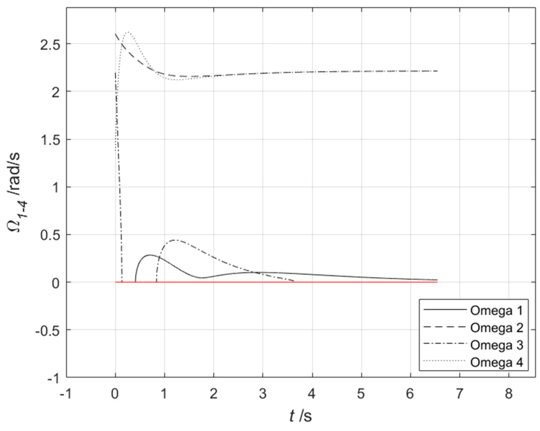
3.3.1. Simulation of the Effectiveness of Dynamic Inverse Decoupling Control

Set the initial coordinate point of the drone to $\left(x_0,y_0,z_0\right)=\left(0,0,0\right)$; the initial attitude angle is $\left({\varphi }_0,{\theta }_0,{\psi }_0\right)=\left(0,0,0\right)$, the initial speed is $\left(v_{x0},v_{y0},v_{z0}\right)=\left(0,0,0\right)$. Since ${\psi }^d$ is set separately, set ${\psi }^d=0.5$. The target point adopts a particle motion model, and the coordinates of the target point are set as $\left(x,y,z\right)=\left(2,2,2\right)$. The angle between the velocity vector and the horizontal plane is set to 0°, and the angle between the horizontal plane projection and the ground x-axis is 30°.

The simulation results of the dynamic inverse decoupling control proposed in this article are as follows:

For the simulation environment of the above parameters and controller parameters, the flight trajectory of the quadcopter drone is shown in Figure 5, and the speed variation is shown in Figure 6. The simulation results show that the drone can accurately reach the set target point:

The changes in control inputs $u_1–u_4$ are shown in Figure 7:

The speed variation of the quadcopter of the drone is shown in Figure 8:

During the flight, the variation in the attitude angles ϕ, θ, and $\psi$ of the quadcopter unmanned aerial vehicle is shown in Figure 9, Figure 10 and Figure 11. Simulation results show that the attitude angle of the unmanned aerial vehicle can eventually converge.

The flight energy consumption of unmanned aerial vehicles under dynamic decoupling control is shown in Figure 12. The dashed line represents instantaneous energy consumption, and the solid line represents total flight energy consumption.

Regarding the sliding mode controller proposed in reference [34], the drone parameters are shown in Table 2. Under the same conditions, the drone flight energy consumption in the sliding mode controller of reference [34] is shown in Figure 13, where the dashed line represents instantaneous energy consumption and the solid line represents total flight energy consumption.

For the classic PID control method, the parameters of the drone are shown in Table 2, and the PID parameters are shown in

Table 4. PID Parameter values.

Variable	Value
${\mathit{K}}_{\mathit{px}}={\mathit{K}}_{\mathit{py}}={\mathit{K}}_{\mathit{pz}}$	0.75
${\mathit{K}}_{\mathit{dx}}={\mathit{K}}_{\mathit{dy}}={\mathit{K}}_{\mathit{dz}}$	1.5
${\mathit{K}}_{\mathit{ix}}={\mathit{K}}_{\mathit{iy}}={\mathit{K}}_{\mathit{iz}}$	0.0
${\mathit{K}}_{\mathit{p}\mathit{\varphi }}={\mathit{K}}_{\mathit{p}\mathit{\theta }}$	15.0
${\mathit{K}}_{\mathit{d}\mathit{\varphi }}={\mathit{K}}_{\mathit{d}\mathit{\theta }}$	6.0
${\mathit{K}}_{\mathit{i}\mathit{\varphi }}={\mathit{K}}_{\mathit{i}\mathit{\theta }}$	1.5
${\mathit{K}}_{\mathit{p}\mathit{\psi }}$	7.5
${\mathit{K}}_{\mathit{d}\mathit{\psi }}$	3.0
${\mathit{K}}_{\mathit{i}\mathit{\psi }}$	0.0

. Under the same conditions, the energy consumption of the drone during flight is shown in Figure 14, where the dashed line represents instantaneous energy consumption and the solid line represents total flight energy consumption.

Based on Figure 12, Figure 13 and Figure 14, the flight energy consumption of unmanned aerial vehicles can be obtained under dynamic inverse decoupling control, the sliding mode controller in reference [34], and classical PID control. In order to better compare and reflect the energy consumption optimization control effect of this article, the comparison chart of flight energy consumption under three states is shown in Figure 15.

The simulation results show that the dynamic inverse decoupling control proposed in this paper can effectively save flight time and energy consumption under three control states, proving the effectiveness and low-energy control characteristics of the proposed decoupling control scheme.

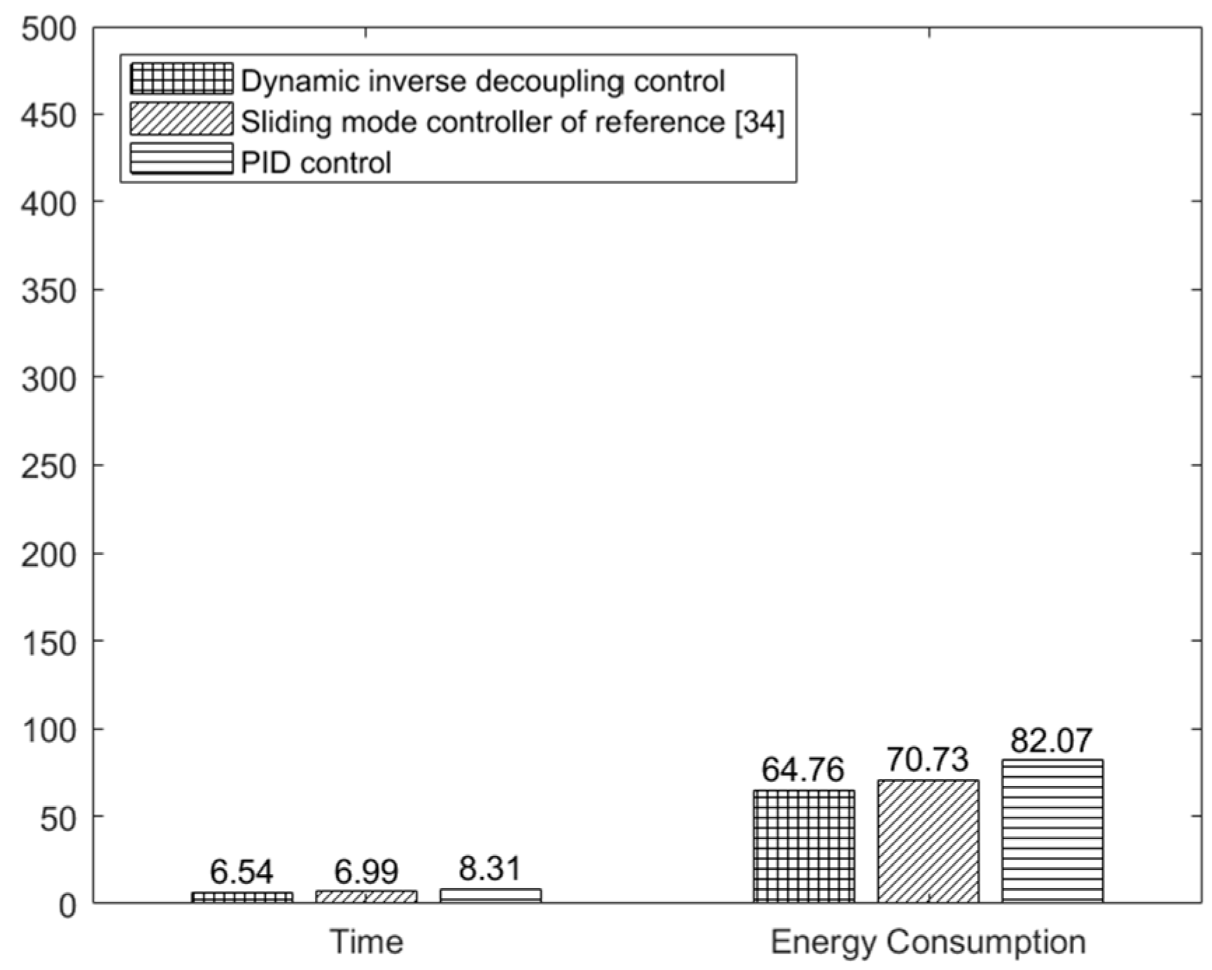
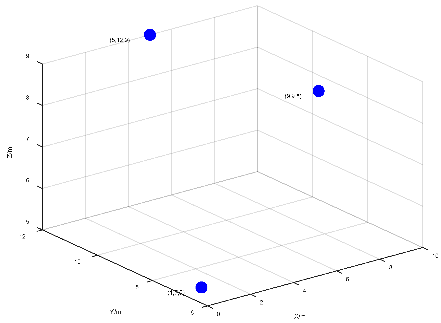
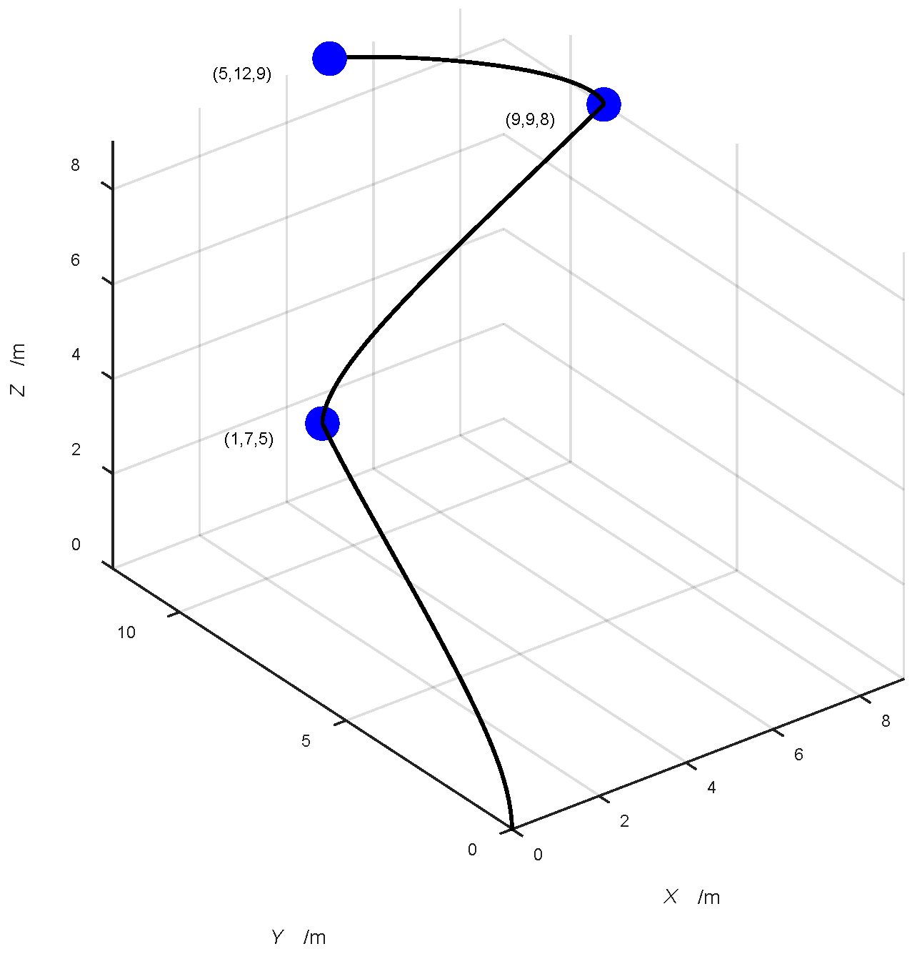
3.3.2. Simulation of the Effectiveness of Energy Optimization in Task Scenarios

In order to verify the effectiveness of the proposed dynamic decoupling control in the task scenario of integrated air–ground cooperation, simulation verification was conducted according to the set scenario and the above simulation steps and conditions.

Assuming there are three sensor nodes, the drone needs to start from the starting point and pass through three sensors in sequence for information collection or charging tasks. The sensor distribution is shown in Figure 16.

According to the conditions and steps set in Section 3.3.1, the simulation was performed, and the obtained drone flight path is shown in Figure 17.

The energy consumption of unmanned aerial vehicle flight under the same simulation and three control algorithms is shown in

Table 5. Three control algorithms for drone flight energy consumption.

Control Algorithm	Total Flight Energy Consumption
Dynamic inverse decoupling control	150.9359 J
Sliding mode controller of reference [34]	311.7295 J
PID control	1500.9461 J

.

It can be seen that in the scenario of integrated air–ground collaborative tasks, the dynamic inverse decoupling control strategy proposed in this paper can still effectively reduce flight energy consumption and achieve energy optimization, verifying the effectiveness of the dynamic inverse decoupling control strategy under integrated air–ground collaboration.

3.4. Actual Flight Test

In order to better verify the practicality of the control method proposed in this paper, the dynamic inverse control, the sliding mode control in reference [34], and the PID control were loaded into the UAV, respectively, for actual flight tests. The actual flight test scenario is shown in Figure 18.

Under the three control methods, the drone reaches the same target point from the same starting point. The initial power of the drone is uniformly set to 100%, and the remaining power after completing the flight mission is shown in

Table 6. Drone remaining battery.

Control Algorithm	Remaining Power
Dynamic inverse decoupling control	78.4%
Sliding mode controller of reference [34]	76.2%
PID control	74.4%

.

Through the comparison of remaining power, it can be seen that the dynamic inverse decoupling control method proposed in this paper can still reduce flight energy consumption in actual flight tests, which proves the practicality of the dynamic inverse decoupling control method.

4. Conclusions and Outlook

Based on the demand for energy consumption optimization of quadcopter unmanned aerial vehicles, this paper proposes a dynamic inverse decoupling control scheme to reduce its control energy consumption and achieve decoupling of motion channels. Firstly, by designing a direct closed-loop feedback control for the z-axis channel, it can exhibit an adjustable second-order linear dynamic response. Then, specific functions of pitch angle and yaw angle are combined as virtual control variables for decoupling the design of the x-axis and y-axis channels, enabling both to have adjustable second-order linear dynamic characteristics. Afterwards, this article designed a calculation method for actual control variables to dynamically and quickly converge the deviation of virtual control variables to the desired value, ensuring control accuracy.

By comparing with other control methods (such as classical PID) in energy consumption simulation, the superiority and control performance of the proposed scheme in energy consumption have been verified, providing new ideas for low-energy control of quadcopter drones.

Likewise, the control algorithm proposed in this paper may have limitations, such as computational complexity issues, which may slightly affect the efficiency of the calculation.

The next step will be to establish an energy consumption model that takes into account environmental dynamic disturbances to increase the practicality of the model. After introducing environmental disturbances, further simplification or improvement of the model can be considered for complex environments (such as strong winds and high temperatures).

Different operators have different styles in controlling the flight attitude and speed of drones, which will also cause energy consumption differences. For example, high-frequency speed changes (such as frequent acceleration and deceleration, and turning) will significantly increase energy consumption; unstable control of flight altitude will easily cause power waste; and too many emergency commands will easily trigger high-load actions. Therefore, reducing human intervention through intelligent auxiliary control can reduce unnecessary energy consumption.

Overall, the dynamic inverse decoupling control method proposed in this paper effectively reduces the flight energy consumption and thus improves the energy efficiency, while addressing the limitation of the traditional method with severe coupling. However, the computational efficiency and the stability of the algorithm against disturbances may pose challenges to the nonlinear control technique using dynamic inverse decoupling. The certification of dynamic inverse decoupling control techniques is also problematic within the aeronautical framework, where the technique is not strictly coupled to AI: this poses a challenge for the adoption of large vehicles such as air taxis.

References

1. Li, X.; Huang, G.; Wang, Z.; Zhao, B. Optics-driven drone. Sci. China Inf. Sci. 2024, 67, 124201. [Google Scholar] [CrossRef]
2. Bartolomei, L.; Teixeira, L.; Chli, M. Fast Multi-UAV Decentralized Exploration of Forests. IEEE Robot. Autom. Lett. 2023, 8, 5576–5583. [Google Scholar] [CrossRef]
3. Bassolillo, S.R.; D’Amato, E.; Notaro, I. A Consensus-Driven Distributed Moving Horizon Estimation Approach for Target Detection Within Unmanned Aerial Vehicle Formations in Rescue Operations. Drones 2025, 9, 127. [Google Scholar] [CrossRef]
4. Jiang, C.X.; Yang, L.A.; Gao, Y.Q.; Zhao, J.; Hou, W.N.; Xu, F.M. An Intelligent 5G Unmanned Aerial Vehicle Path Optimization Algorithm for Offshore Wind Farm Inspection. Drones 2025, 9, 47. [Google Scholar] [CrossRef]
5. Rad, S.S.; Zheng, Z.; Kheirollahi, R.; Mostafa, A.; Zhao, S.; Wang, Y.; Chevinly, J.; Nadi, E.; Bensala, T.; Zhang, H.; et al. Electromagnetic Interference on Unmanned Aerial Vehicles (UAVs): A Case Study of High Power Transmission Line Impacts. IEEE Trans. Transp. Electrif. 2025, 1. [Google Scholar] [CrossRef]
6. Ahmed, M.; Soofi, A.A.; Raza, S.; Khan, F.; Ahmad, S.; Ullah, W.; Asif, M.; Xu, F.; Han, Z. Advancements in RIS-Assisted UAV for Empowering Multi-Access Edge Computing: A Survey. IEEE Internet Things J. 2025, 12, 6325–6346. [Google Scholar] [CrossRef]
7. Cao, P.; Lei, L.; Cai, S.; Shen, G.; Liu, X.; Wang, X.; Zhang, L.; Zhou, L.; Guizani, M. Computational Intelligence Algorithms for UAV Swarm Networking and Collaboration: A Comprehensive Survey and Future Directions. IEEE Commun. Surv. Tutor. 2024, 26, 2684–2728. [Google Scholar] [CrossRef]
8. Xu, S.; Zou, N.; He, Q.; He, X.; Li, K.; Cheng, M.; Liu, K. Design and Application Research of a UAV-Based Road Illuminance Measurement System. Automation 2024, 5, 407–431. [Google Scholar] [CrossRef]
9. Lang, M.; Antsov, M.; Mumma, A.; Suitso, I.; Kuusk, A.; Piip, K. Comparison of forest canopy gap fraction measurements from drone-based video frames, below-canopy hemispherical photography, and airborne laser scanning. Eur. J. Remote Sens. 2025, 58, 2456629. [Google Scholar] [CrossRef]
10. Qu, H.; Zheng, C.; Ji, H.; Barai, K.; Zhang, Y.-J. A fast and efficient approach to estimate wild blueberry yield using machine learning with drone photography: Flight altitude, sampling method and model effects. Comput. Electron. Agric. 2024, 216, 108543. [Google Scholar] [CrossRef]
11. Ri, S.; Ye, J.; Xia, P.; Toyama, N.; Ogura, N.; Shiotani, T. Bridge deflection measurement by drone aerial photography using the sampling moiré method. In Proceedings of the International Conference on Optical and Photonic Engineering (icOPEN 2023), Singapore, 15 February 2024; pp. 168–171. [Google Scholar]
12. Gao, J.; Wang, Q.; Li, Z.; Zhang, X.; Hu, Y.; Han, Q.; Pan, Y. Toward Efficient Urban Emergency Response Using UAVs Riding Crowdsourced Buses. IEEE Internet Things J. 2024, 11, 22439–22455. [Google Scholar] [CrossRef]
13. De Lucia, L.; Palazzi, C.E.; Vegni, A.M. ENSING: Energy saving based data transmission in Internet of Drones for 3D connectivity in 6G networks. Ad Hoc Netw. 2023, 149, 103211. [Google Scholar] [CrossRef]
14. Cariou, C.; Moiroux-Arvis, L.; Bendali, F.; Mailfert, J. Optimal route planning of an Unmanned Aerial Vehicle for data collection of agricultural sensors. In Proceedings of the IEEE INFOCOM 2024-IEEE Conference on Computer Communications Workshops (INFOCOM WKSHPS), Vancouver, BC, Canada, 20 May 2024; pp. 1–6. [Google Scholar]
15. Wu, Y.; Yin, H.; Chen, X.; Zhang, M. Multicircuit Route Planning for UAVs Performing the Terrain Coverage Task. IEEE Internet Things J. 2024, 11, 23765–23779. [Google Scholar] [CrossRef]
16. Alyassi, R.; Khonji, M.; Karapetyan, A.; Chau, S.C.K.; Elbassioni, K.; Tseng, C.M. Autonomous Recharging and Flight Mission Planning for Battery-Operated Autonomous Drones. IEEE Trans. Autom. Sci. Eng. 2023, 20, 1034–1046. [Google Scholar] [CrossRef]
17. Wan, P.; Wang, S.; Xu, G.; Long, Y.; Hu, R. Hybrid Heuristic-Based Multi-UAV Route Planning for Time-Dependent Data Collection. IEEE Internet Things J. 2024, 11, 24134–24147. [Google Scholar] [CrossRef]
18. Wang, X.; Ma, T.; Zhang, L.; Qiao, N.; Xue, P.; Fu, J. Multi-Phase Trajectory Planning for Wind Energy Harvesting in Air-Launched UAV Swarm Rendezvous and Formation Flight. Drones 2024, 8, 709. [Google Scholar] [CrossRef]
19. Hadid, S.; Boushaki, R.; Boumchedda, F.; Merad, S. Enhancing Quadcopter Autonomy: Implementing Advanced Control Strategies and Intelligent Trajectory Planning. Automation 2024, 5, 151–175. [Google Scholar] [CrossRef]
20. Perrusquia, A.; Guo, W. Reservoir Computing for Drone Trajectory Intent Prediction: A Physics Informed Approach. IEEE Trans. Cybern. 2024, 54, 4939–4948. [Google Scholar] [CrossRef]
21. Zhuang, X.; Li, D.; Wang, Y.; Liu, X.; Li, H. Optimization of high-speed fixed-wing UAV penetration strategy based on deep reinforcement learning. Aerosp. Sci. Technol. 2024, 148, 109089. [Google Scholar] [CrossRef]
22. Carvajal, C.P.; Andaluz, V.H.; Varela-Aldás, J.; Roberti, F.; Del-Valle-Soto, C.; Carelli, R. Visual Servoing Using Sliding-Mode Control with Dynamic Compensation for UAVs’ Tracking of Moving Targets. Drones 2024, 8, 730. [Google Scholar] [CrossRef]
23. Kumar, S.; Yesmin, A.; Sinha, A.; Guha, A. Adaptive Continuous Terminal Sliding Mode Control for Unmanned Aerial Vehicle. In Proceedings of the 2024 Tenth Indian Control Conference (ICC), Bhopal, India, 9–11 December 2024; pp. 262–267. [Google Scholar]
24. Admas, Y.A.; Mitiku, H.M.; Salau, A.O.; Omeje, C.O.; Braide, S.L. Control of a fixed wing unmanned aerial vehicle using a higher-order sliding mode controller and non-linear PID controller. Sci. Rep. 2024, 14, 23139. [Google Scholar] [CrossRef] [PubMed]
25. Yu, H.; Miao, K.; He, Z.; Zhang, H.; Niu, Y. Fault-Tolerant Time-Varying Formation Trajectory Tracking Control for Multi-Agent Systems with Time Delays and Semi-Markov Switching Topologies. Drones 2024, 8, 778. [Google Scholar] [CrossRef]
26. Lee, B.; Hyun, D.; Kim, J.; Lee, S.; Ban, J. Design of Robust H∞ Guaranteed Cost Controller of Quadrotor UAV for Set-Point Tracking. IEEE Access 2024, 12, 126074–126087. [Google Scholar] [CrossRef]
27. Xing, S.; Zhang, X.; Tian, J.; Xie, C.; Chen, Z.; Sun, J. Morphing Quadrotors: Enhancing Versatility and Adaptability in Drone Applications—A Review. Drones 2024, 8, 762. [Google Scholar] [CrossRef]
28. Wu, Y.; Chen, M.; Li, H.; Chadli, M. Event-Triggered-Based Adaptive NN Cooperative Control of Six-Rotor UAVs With Finite-Time Prescribed Performance. IEEE Trans. Autom. Sci. Eng. 2024, 21, 1867–1877. [Google Scholar] [CrossRef]
29. Liu, S.; Jiang, B.; Mao, Z.; Zhang, Y. Distributed adaptive event-triggered fault-tolerant cooperative control of multiple UAVs and UGVs under DoS attacks. IET Contr. Theory Appl. 2023, 18, 2296–2306. [Google Scholar] [CrossRef]
30. Amertet, S.; Gebresenbet, G.; Alwan, H.M. Modeling of Unmanned Aerial Vehicles for Smart Agriculture Systems Using Hybrid Fuzzy PID Controllers. Appl. Sci. 2024, 14, 3458. [Google Scholar] [CrossRef]
31. Tassanbi, A.; Ali Khan, A.; Kashkynbayev, A.; Shehab, E.; Duc Do, T.; Ali, M.H. Performance evaluation of developed controllers for unmanned aerial vehicles with reference camera. Meas. Control 2024, 2, 00202940241270863. [Google Scholar] [CrossRef]
32. Zhao, H.; Fu, H.; Yang, F.; Qu, C.; Zhou, Y. Data-driven offline reinforcement learning approach for quadrotor’s motion and path planning. Chin. J. Aeronaut. 2024, 37, 386–397. [Google Scholar] [CrossRef]
33. Yao, J.; Rafee Nekoo, S.; Xin, M. Approximate optimal control design for quadrotors: A computationally fast solution. Optim. Control Appl. Methods 2023, 45, 85–105. [Google Scholar] [CrossRef]
34. Xiong, J.J.; Zheng, E.H. Position and attitude tracking control for a quadrotor UAV. ISA Trans. 2014, 53, 725–731. [Google Scholar] [CrossRef]
35. Li, B.; Li, Q.; Zeng, Y.; Rong, Y.; Zhang, R. 3D Trajectory Optimization for Energy-Efficient UAV Communication: A Control Design Perspective. IEEE Trans. Wirel. Commun. 2022, 21, 4579–4593. [Google Scholar] [CrossRef]
Figure 1. Quadcopter drone fuselage structure. E(ex, ey, ez) represents the ground coordinate system, B ( x , y , z ) represents the body coordinate system. The lift generated by motors 1 to 4 is given as F 1 to F 4 , respectively. ϕ represents the roll angle of the drone around the x -axis, θ represents the pitch angle of the drone around the y -axis, and ψ represents the yaw angle of the drone around the z -axis; that is, the Euler angle of the quadcopter drone in the Z - Y - X rotation sequence is [ ϕ , θ , ψ ] .
Automation 06 00019 g001
Figure 2. UAV energy consumption measurement scenario.
Automation 06 00019 g002
Figure 3. Changes in drone power and time.
Automation 06 00019 g003
Figure 4. Simulink block diagram used for simulation.
Automation 06 00019 g004
Figure 5. Quadcopter drone flight trajectory.
Automation 06 00019 g005
Figure 6. Speed variation of quadcopter unmanned aerial vehicle.
Automation 06 00019 g006
Figure 7. Control input u1u4 changes.
Automation 06 00019 g007
Figure 8. Rotation speed variation of quadcopter of unmanned aerial vehicle.
Automation 06 00019 g008
Figure 9. Drone ϕ angle change.
Automation 06 00019 g009
Figure 10. Drone θ angle change.
Automation 06 00019 g010
Figure 11. Drone ψ angle change.
Automation 06 00019 g011
Figure 12. Energy consumption of unmanned aerial vehicle flight under dynamic inverse decoupling control.
Automation 06 00019 g012
Figure 13. Sliding mode controller of reference [34]. Energy consumption of unmanned aerial vehicle flight in controller.
Automation 06 00019 g013
Figure 14. Energy consumption of unmanned aerial vehicle flight under classical PID control.
Automation 06 00019 g014
Figure 15. Comparison of flight energy consumption under three control states.
Automation 06 00019 g015
Figure 16. Sensor distribution.
Automation 06 00019 g016
Figure 17. UAV flight path under dynamic inverse decoupling control task scenario.
Automation 06 00019 g017
Figure 18. Actual flight test scene diagram.
Automation 06 00019 g018