Pre-Routing Slack Prediction Based on Graph Attention Network

Abstract

Static Timing Analysis (STA) plays a crucial role in realizing timing convergence of integrated circuits. In recent years, there has been growing research on pre-routing timing prediction using Graph Neural Networks (GNNs). However, existing approaches struggle with scalability on large graphs and lack generalizability to new designs, limiting their applicability to large-scale, complex circuit problems. To address this issue, this paper proposes a timing engine based on Graph Attention Network (GAT) to predict the slack of timing endpoints. Firstly, our model computes net embeddings for each node prior to training using a gated self-attention module. Subsequently, inspired by the Nonlinear Delay Model (NLDM), the node embeddings are propagated through multiple levels by alternately applying net propagation layers and cell propagation layers. Evaluated on 21 real circuits, the framework achieved a 16.62% improvement in average $R^2$ score for slack prediction and a 15.55% reduction in runtime compared to the state-of-the-art (SOTA) method.

1. Introduction

Static timing analysis (STA) plays an important role in chip design. By predicting the post-routing timing in the placement stage, the placer can perform more accurate and effective timing optimization in the placement stage, thus promoting the timing convergence of the circuit. However, as shown in Figure 1, the timing analysis results of existing STA tools are not accurate due to the lack of routing information in the placement phase. This makes the timing optimization in the placement phase less effective, leading to the increase of time cost in the subsequent timing optimization phase and the difficulty of chip timing convergence. Therefore, the research on accurate timing analysis tools has become an important task.

Since circuit netlists can be naturally represented as graphs, the application of a Graph Neural Network (GNN) in STA has rapidly gained attention in recent years [1]. In current research, the prediction of slack is generally improved either directly or indirectly. Some studies enhance net delay prediction by using a look-ahead RC network within the GNN model to extract complete timing features [2,3,4,5]. Other works improve cell delay prediction by assigning multidimensional features to nodes and edges and utilizing GNN to simulate the lookup table process [6,7,8]. Additionally, some studies directly enhance slack prediction by integrating netlist-layout information through multimodal fusion [9,10,11].

Although the use of GNN in STA has shown promising results, existing methods still have notable limitations. First, previous works [7] treated the influence of different cells on net delay prediction equally, overlooking the varying roles of nodes in the propagation process. Second, prior approaches employed overly complex methods to model cell delay calculations, which leads to model overfitting. These limitations ultimately hinder the precision of slack predictions. To address this limitation, this paper proposes a timing prediction framework based on the Graph Attention Network (GAT) and simulated lookup table. The main contributions are summarized as follows:

• We present an end-to-end graph learning framework for predicting pre-routing arrival time and slack values at timing endpoints with no need to invoke additional STA tools.
• We leverage an attention mechanism to capture the importance of interactions between nodes, thereby enhancing the prediction accuracy of net delay.
• Inspired by the Nonlinear Delay Model (NLDM) computation process, our method incorporates the lookup table as a cell feature, addressing the model’s tendency to fall into local optima and improving operational efficiency.
• Results on the 21 real-world circuit benchmarks demonstrate that our method achieves a 16.62% improvement in $R^2$ of slack while reducing runtime by 15.55% compare to the previous state-of-the-art (SOTA) method [7].

2. Literature Survey

2.1. Graph Attention Network Applied to Electronic Design Automation

Unlike traditional Graph Convolutional Networks, GAT leverages the self-attention mechanism to process graph-structured data [12]. GAT adjusts inter-node messaging weights based on feature importance, updating node representations through attention-weighted aggregation of neighbor features. Specifically, the attention coefficient for the node $v_i$ and its neighbor $v_j$ is computed as follows:

$${\alpha }_{ij}={\displaystyle \frac{\exp \left(\mathrm{LeakyReLU}\left({\overrightarrow{a}}^T\left[W{\overrightarrow{h}}_i\parallel W{\overrightarrow{h}}_j\right]\right)\right)}{{\sum }_{k\in {\mathcal{N}}_i}\exp \left(\mathrm{LeakyReLU}\left({\overrightarrow{a}}^T\left[W{\overrightarrow{h}}_i\parallel W{\overrightarrow{h}}_k\right]\right)\right)}}.$$

(1)

where W is the linear transformation matrix and $h_i$ and $h_j$ are the feature representations of nodes $v_i$ and $v_j$, respectively. This allows GAT to adapt the information flow during the aggregation of neighboring node features, improving the model’s expressiveness and flexibility.

In recent years, GAT has been widely adopted in the field of EDA due to their strong expressive capabilities and flexible weight adjustment mechanisms. For example, Ref. [13] introduced a GAT model for estimating delay and area metrics of post-physical synthesis circuits from the netlist of pre-physical synthesis circuits. Ref. [14] proposed a customizable GAT approach to estimate individual net length before cell placement. Refs. [15,16] employed GAT during the placement phase to predict congestion. In the domain of analog circuit design, GAT has also been applied to predict net parasitic capacitances and circuit performance [17,18].

The aforementioned works demonstrate the broad application of GAT in the EDA field, with results consistently surpassing traditional methods. However, no existing work has applied GAT to timing prediction during the placement stage. This gap affects the accuracy of circuit modeling and consequently limits the effectiveness of timing prediction.

2.2. Machine Learning Applied to Static Timing Analysis

STA verifies whether a design can operate at a specified frequency by analyzing the design alongside input clock definitions and the external environment parameters [19]. To calculate net delay, STA employs the wire load model and the Elmore delay model. The wire load model estimates the RC parameters of a net based on library data, while the Elmore delay model computes net delay using these parameters. For cell delay, STA often employs the NLDM model to perform timing checks across various timing arcs [19]. The NLDM model determines cell delay as a function of two independent variables: input transition time and output load capacitance. When a table entry is unavailable, STA applies two-dimensional interpolation to estimate the final timing value.

After calculating the net delay and cell delay, STA iteratively computes the arrival time (AT), which is defined as the moment when a signal reaches the pin, starting from the primary input (PI). Similarly, the required arrival time (RAT) is defined as the constraint imposed on each AT to maintain the clock frequency, starting from the primary output (PO). With RAT and AT defined, the slack is then calculated as follows:

$$slac{k}^E=A{T}^E-RA{T}^E,slac{k}^L=RA{T}^L-A{T}^L.$$

(2)

where E means early, L means late, a positive slack indicates that the timing constraint is satisfied, and a negative slack indicates that there is a timing violation in the circuit.

In recent years, many attractive GNN models [20,21,22,23] have been proposed. These methods further demonstrate the strong capability of GNN in structural modeling and feature representation. As a result, GNN have been widely applied to Electronic Design Automation (EDA) field for timing prediction [24]. Ref. [7] proposed a GNN-inspired timing engine that treats edge delays as a local auxiliary task to enhance the accuracy of predicted arrival time and timing endpoint slack. In this approach, a lookup table (LUT) interpolation module simulates the cell delay lookup process, generating and propagating wire mesh/cell embeddings in topological order. Ref. [8] proposed a timing prediction method that simulates the calculation process of STA. The proposed method introduces global circuit training and proposes a graph autoencoder that learns global graph embeddings from the circuit netlist, further improving the accuracy of predicted arrival time and slack.

The above research proves the effectiveness of machine learning technology in pre-routing timing prediction. Unfortunately, Refs. [7,8] do not account for the varying influence of cells on timing prediction in practical circuits, primarily due to the complexity of resistance and capacitance modeling. This oversight results in suboptimal net delay prediction performance. At the same time, these works simulate both LUT and interpolation algorithms for cell delay prediction, significantly increasing model complexity and ultimately leading to overfitting, which limits the effectiveness of cell delay prediction.

3. Proposed Methods

3.1. Overall Flow

In our timing prediction framework, the placed circuit is represented as a heterogeneous graph with two types of edges. The nodes correspond to cell pins, while the edges, classified as net or cell edges, distinguish the two types of timing arcs used in STA analysis. Inspired by the STA process, our framework is divided into two parts: net embedding and delay propagation, as shown in Figure 2. In the net embedding model, convolutional layers update the features of net drivers and sinks to calculate net delay. In the delay propagation model, features are propagated through net and cell layers to predict cell delay, slew, and arrival time.

Meanwhile, we briefly describe the workflow of the proposed method through Algorithm 1, which is divided into four parts:

• Lines 4 to 10 outline the process of updating sink node features: The driver node feature $f_d$, the sink node feature $f_s$, and the edge feature $f_{d\to s}$ are weighted by the weight matrix $w_{i,j}$, concatenated and passed through the MLP to obtain the new feature $F_s$ of the sink node.
• Lines 11 through 20 outline the process of updating the driver node features: The driver node feature $f_d$, the sink node feature $f_s$, and the edge feature $f_{s\to d}$ from the sink node to the driver node are weighted by the weight matrix $w_{i,j}$, and concatenated to obtain the new features $F_1$ and $F_2$ by MLP. Then, weighting it again with the driver node feature $f_d$, concatenating it and passing it through the MLP, we obtain the new feature $F_d$ of the driver node.
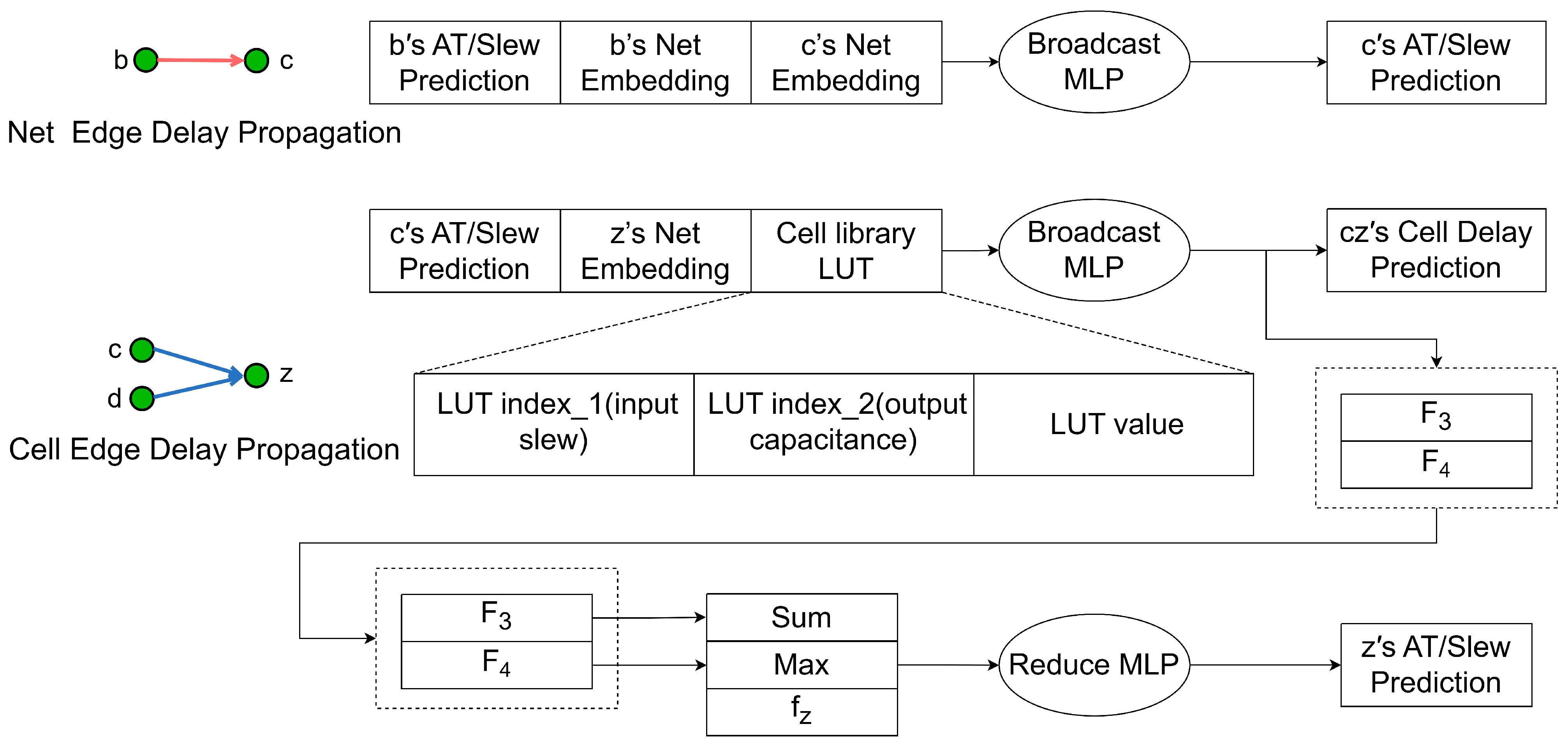
• Lines 21 to 23 describe the prediction process for arrival times and slew along net edges: By concatenating the arrival time $A{T}_d$ of the driver node, the slew $Sle{w}_d$, the new feature $F_d$ of the driver node, and the new feature $F_s$ of the sink node and passing it through the MLP, we obtain the arrival time $A{T}_s$ and slew $Sle{w}_s$ of the sink node.
• Lines 24 to 30 outline the prediction process for arrival times and turns along cell edges: Firstly, the LUT value is found by cell slew and capacitance, and then the three are concatenated to obtain the cell edge feature $f_{d\to s}$. Then, the arrival time $A{T}_d$ of the driver node, the slew $Sle{w}_d$, the new feature of the sink node $F_s$, and the cell edge feature $f_{d\to s}$ are concatenated and passed through the MLP to obtain the new features $F_3$, $F_4$ and the cell delay. Finally, $F_3$ is summed up, $F_4$ takes the maximum value and concatenates the features $f_s$ of the sink node and passes it through MLP. We can obtain the arrival time $A{T}_s$ and slew $Sle{w}_s$ of the sink node.

Algorithm 1 Graph-based delay prediction with attention and LUT
1:	Input: Circuit Graph $G(V,E)$, Netlist N, Cell Library $LUT$
2:	Output: Arrival time/slew Prediction for sink Nodes $F_s$
3:	Initialization: Initialize node features $f_x$ for each $x\in V$
4:	for each sink node $s\in V$ do	▹ Graph Broadcast Phase
5:	for each diver node $d\in V$ do
6:	$w_{i,j}\leftarrow \mathrm{Attention}(f_d,f_s,f_{d\to s})$
7:	$f_d^{\prime },f_s^{\prime },f_{d\to s}^{\prime }\leftarrow \left(w_{i,j}\right)\ast (f_d\left|\right|f_s\left|\right|f_{d\to s})$
8:	$F_s\leftarrow \mathrm{Broadcast}\mathrm{MLP}(f_d^{\prime },f_s^{\prime },f_{d\to s}^{\prime })$
9:	end for
10:	end for
11:	for each diver node $d\in V$ do	▹ Graph Reduction Phase
12:	for each sink node $s\in V$ do
13:	$w_{i,j}\leftarrow \mathrm{Attention}(f_d,f_s,f_{s\to d})$
14:	$f_d^{\prime },f_s^{\prime },f_{s\to d}^{\prime }\leftarrow \left(w_{i,j}\right)\ast (f_d,f_s,f_{s\to d})$
15:	$F_1,F_2\leftarrow \mathrm{Broadcast}\mathrm{MLP}(f_d^{\prime }\left|\right|f_s^{\prime }\left|\right|f_{s\to d}^{\prime })$
16:	$w_{i,j}\leftarrow \mathrm{Attention}(F_1,F_2,f_d)$
17:	$F_1^{\prime },F_2^{\prime },f_d^{\prime }\leftarrow \left(w_{i,j}\right)\ast (F_1,F_2,f_d)$
18:	$F_d\leftarrow \mathrm{Reduce}\mathrm{MLP}(SUM\left(F_1^{\prime }\right)\left|\right|MAX\left(F_2^{\prime }\right)\left|\right|f_d^{\prime })$
19:	end for
20:	end for
21:	for each net edge $(d\to s)$ do	▹ Net Edge Delay Propagation
22:	$A{T}_s,Sle{w}_s\leftarrow \mathrm{Broadcast}\mathrm{MLP}(A{T}_d\left|\right|Sle{w}_d\left|\right|F_d\left|\right|F_s)$
23:	end for
24:	for each cell edge $(d\to s)$ do	▹ Cell Edge Delay Propagation
25:	$LUTvalue\leftarrow LUT\left[\mathrm{index}(Sle{w}_c,Ca{p}_c)\right]$
26:	$f_{d\to s}\leftarrow (Sle{w}_c\left|\right|Ca{p}_c\left|\right|LUTvalue)$
27:	$F_3,F_4,Cell\_dela{y}_c\leftarrow \mathrm{Broadcast}\mathrm{MLP}(A{T}_d\left|\right|Sle{w}_d\left|\right|F_s\left|\right|f_{d\to s})$
28:	$A{T}_s,Sle{w}_s\leftarrow \mathrm{Reduce}\mathrm{MLP}(SUM\left(F_3\right)\left|\right|MAX\left(F_4\right)\left|\right|f_s)$
29:	end for
30:	Return $A{T}_s,Sle{w}_s$

3.2. Net Embedding Model

During the net embedding process, previous work [7] propagated information uniformly from neighboring nodes through GCN, without giving sufficient attention to the most relevant input components through attention mechanism or other methods. However, in the process of net delay prediction, capacitance models are often simplified, and resistance is frequently neglected [25]; this simplification changes the charging and discharging waveforms of the net in the circuit, making the importance of nodes and edges no longer consistent, which directly leads to the inaccurate net delay prediction.

To solve this problem, we incorporate an attention mechanism into our model. This mechanism allows the model to adaptively learn the actual relationships between node and edge features [12], assigning weights that capture the true impact of resistance and capacitance on the delay prediction. Since cell delay does not directly affect the net delay prediction result, only net drivers and their neighboring sinks participate in the embedding process, which leads to the fact that the calculation of net delay in our model is only related to the information of neighbor nodes. Therefore, we use local attention in GAT to weight neighbor node features.

As shown in Figure 3, our net embedding model consists of network convolutional layers with two steps: graph broadcasting and graph reduction. In the graph broadcasting step, we aim to compute new features for the net sink. Firstly, for the features $f_d$, $f_s$ and $f_{d\_s}$ of net drivers, net sinks and net edges, we calculate the attention coefficients for the nodes and edges using a linear layer and normalize them. Then, we weighted the features according to the attention coefficients $w_1$, $w_2$, and $w_3$ to obtain the new updated features $f_d^{\prime }$, $f_s^{\prime }$, and $f_{d\_s}^{\prime }$:

$$f_d^{\prime }=w_1\ast f_d,f_s^{\prime }=w_2\ast f_s,f_{d\_s}^{\prime }=w_3\ast f_{d\_s}.$$

(3)

By concatenating the weighted features and passing them through an MLP, we obtain the updated feature $F_s$ for the net sink:

$$F_s=ML{P}_{d\_s}(f_d^{\prime }\left|\right|f_s^{\prime }\left|\right|f_{d\_s}^{\prime })$$

(4)

In the graph reduction step, we aim to compute new features for net drivers. Similar to graph broadcasting, we weight the features to obtain updated features $f_s^{\prime }$,$f_d^{\prime }$,$f_{s\_d}^{\prime }$, then output two equal-length subtensors, $F_1$ and $F_2$, through an MLP:

$$F_1,F_2=split(ML{P}_{s\_d}(f_s^{\prime }\left|\right|f_d^{\prime }\left|\right|f_{s\_d}^{\prime }\left)\right)$$

(5)

Next, we apply the $SUM$ and $MAX$ operations to the two subtensors, $F_1$ and $F_2$, where the $SUM$ operation simulates the STA computational cell output load, and the $MAX$ identifies the most influential features. After weighting these two sets of information along with the net driver features to obtain updated features $F_1^{\prime }$ and $F_2^{\prime }$, we concatenate them and reduce the dimensionality through an MLP to obtain the new net driver feature $F_d$:

$$F_d=ML{P}_{reduce}({\sum }_{s\in N_d}\left(F_1^{\prime }\right)\left|\right|MA{X}_{s\in N_d}\left(F_2^{\prime }\right)\left|\right|f_d^{\prime }).$$

(6)

These updated net sink and net driver features are passed through two additional network convolutional layers, from which we obtain the net delay from the net driver to the net sink.

3.3. Delay Propagation Model

Cell delay refers to the delay introduced as a signal passes through the logic cells in a circuit. This delay impacts the overall timing of the circuit and, along with net delay, determines the signal’s arrival time. Accurate prediction of cell delay is crucial for timing optimization, as it directly influences the precision of timing analysis, which in turn affects the performance and convergence of the circuit design.

In cell delay prediction, the calculation process of the NLDM model is relatively complex. As a result, simulating the NLDM model can cause the model to learn noise and outliers in the training data. Since these learned patterns do not generalize well to new datasets, the final prediction accuracy suffers [26]. To solve this problem, we directly use the lookup table index as an input feature and remove the interpolation process learned by the MLP. As shown in Figure 4, the net delay propagation layer operates similarly to graph broadcasting. We concatenate the arrival time/slew value $A{S}_d$ with the net driver $F_d$ and net sink features $F_s$, and then use the MLP to calculate the predicted arrival time/slew value $A{S}_s$ for the net sink:

$$A{S}_s=ML{P}_{board}(A{S}_d\left|\right|F_d\left|\right|F_s)$$

(7)

In the cell delay propagation layer, we concatenate the features required for the cell LUT, including the predicted value $A{S}_d$ from the net driver, the features $F_s$ of the net sink, and the LUT information $f_{d\_s}$ provided by the cell edges. The LUT information consists of input transition time, output load capacitance, and delay value. These concatenated features are then passed through an MLP, which decomposes them into two subtensors of equal length: $F_3$, $F_4$, and the delay of the cell edge, $C{D}_{d\_s}$.

$$F_3,F_4,C{D}_{d\_s}=split(ML{P}_{board}(A{S}_d\left|\right|F_s\left|\right|f_{d\_s}\left)\right).$$

(8)

After performing the $SUM$ and $MAX$ operations on the computed cell arc messages, we concatenate these messages with the net sink feature $F_s$. Passing this combined input through the MLP yields the predicted arrival time and slew value, denoted as $A{S}_s$, for the net sink:

$$A{S}_s=ML{P}_{reduce}({\sum }_{s\in N_d}\left(F_3\right)\left|\right|MA{X}_{s\in N_d}\left(F_4\right)\left|\right|F_s)$$

(9)

4. Results

4.1. Experimental Setup

We build our framework with PyTorch [27] and DGL [28] on a 64-bit Linux machine with two 2.60 GHz Intel Xeon CPU with 28 cores, 1 NVIDIA GeForce RTX 4090 GPUs, and 24 GB RAM. Our net embedding model contains a total of three network convolutional layers, and the MLP in all models has three hidden layers, with a hidden layer dimension of 64. For fairness, we adopt the same features and dataset settings as in [7].

Table 1. Benchmark statistics.

	Name	Nodes	Nets	Cells	Endpoints
Train	blabla	55,568	39,853	35,689	1614
	usb_cdc_core	7406	5200	4869	630
	BM64	38,458	27,843	25,334	1800
	salsa20	78,486	57,737	52,895	3710
	aes128	211,045	148,997	138,457	5696
	wbqspiflash	9672	6798	6454	323
	cic_decimator	3131	2232	2102	130
	aes256	290,955	207,414	189,262	11,200
	des	60,541	44,478	41,845	2048
	aes_cipher	59,777	42,671	41,411	660
	picorv32a	58,676	43,047	40,208	1920
	zipdiv	4398	3102	2913	181
	genericfir	38,827	28,845	25,013	3811
	usb	3361	2406	2189	344
Test	jpeg_encoder	23,8216	17,6737	16,7960	4422
	usbf_device	66,345	46,241	42,226	4404
	aes192	234,211	165,350	152,910	8096
	xtea	10,213	7151	6882	423
	spm	1121	765	700	129
	y_huff	48,216	33,689	30,612	2391
	synth_ram	25,910	19,024	16,782	2112

shows the information of the benchmark we used in the experiments, where the size of the training set ranges from 3 k cells to 290 k cells and the size of the test set ranges from 1 k cells to 240 k cells. All timing reports were generated by OpenROAD on SkyWater 130 nm technology, and these data are all accessible in the gitHub repository. OpenROAD is an open source EDA tool that integrates logic synthesis, timing analysis, placement, and routing.

For evaluation, we utilize the $R^2$ coefficient of determination score to measure prediction performance:

$$R^2=1-{\displaystyle \frac{\frac{1}{n}{\sum }_{i=1}^n{(y_i-{\widehat{y}}_i)}^2}{\frac{1}{n}{\sum }_{i=1}^n{(y_i-\overline{y})}^2}}=1-{\displaystyle \frac{\mathrm{MSE}(\mathbf{y},\widehat{\mathbf{y}})}{\mathrm{VAR}\left(\mathbf{y}\right)}}$$

(10)

where $y_i$ represents the true values, $\widehat{y}$ denotes the prediction value, and $\overline{y}$ is the mean of the true values. In addition, MSE (Mean Squared Error) is also used as an evaluation index to evaluate the accuracy of the proposed model in timing prediction.

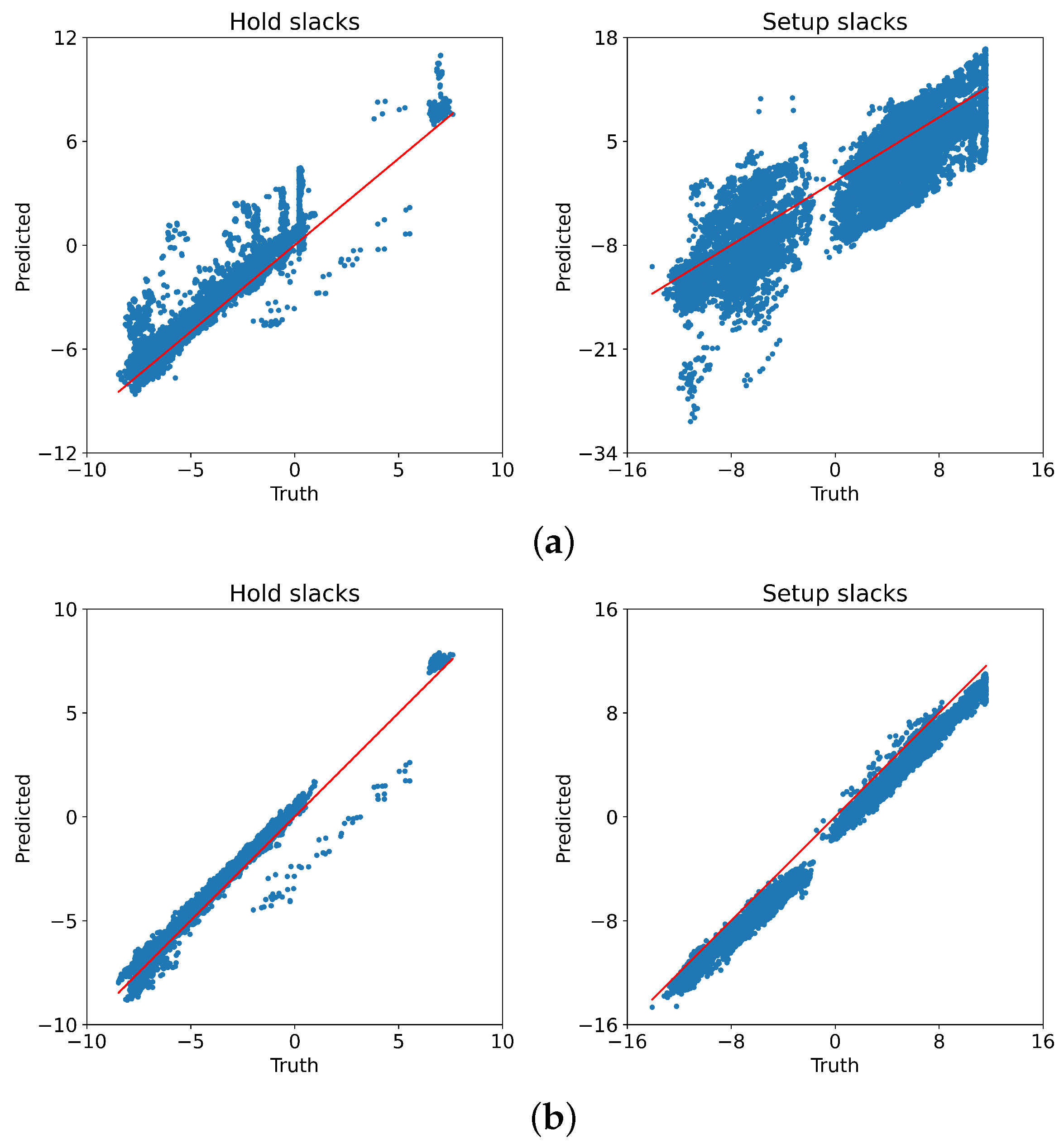
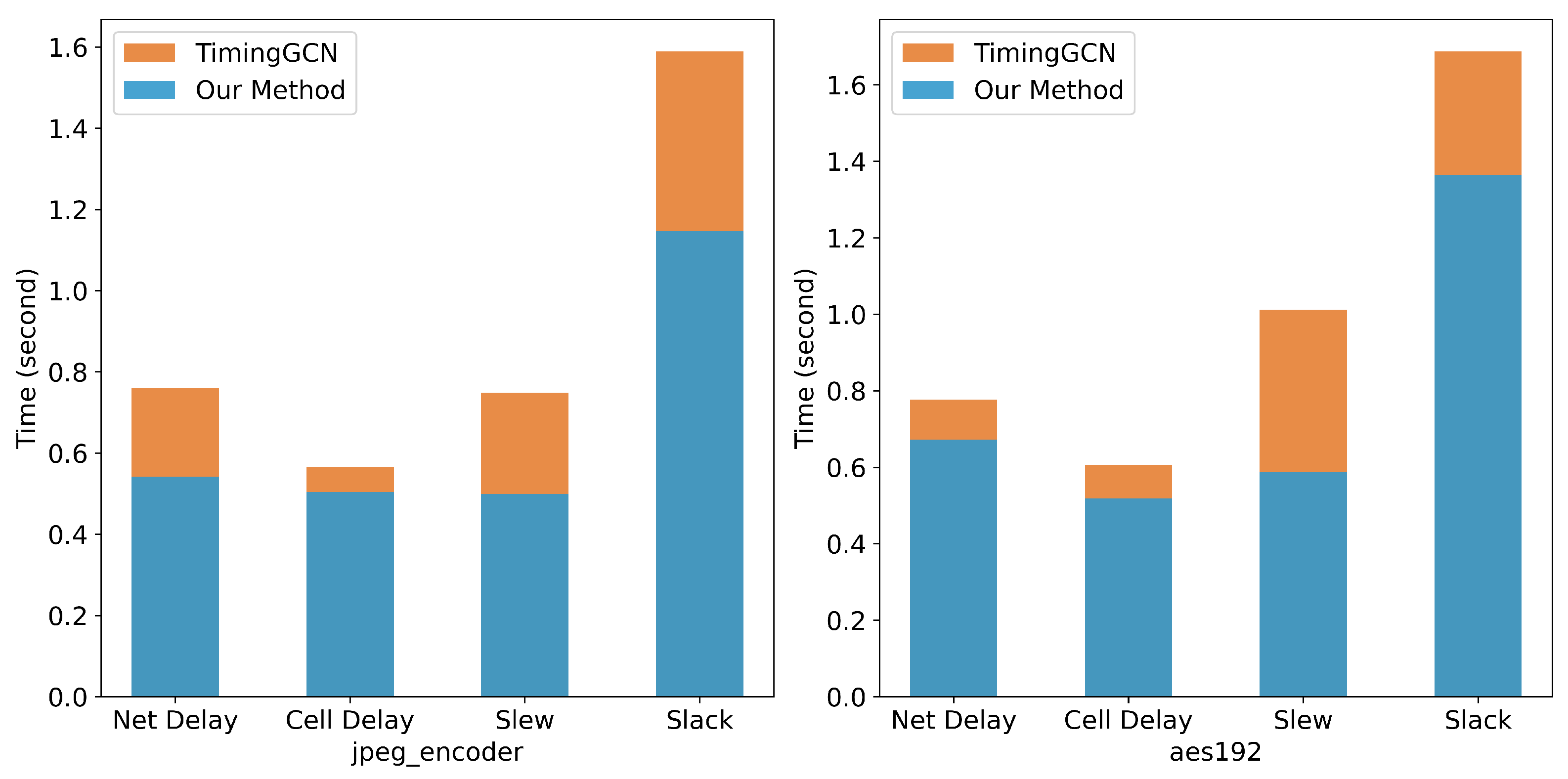
4.2. Timing Prediction Results

We compare the proposed method with the pre-route timing evaluation method presented in [7].

Table 2. Comparison with Ref. [7] on the test set, including net delay and cell delay.

	Benchmark	Net Delay (${\mathit{R}}^2$ Score)			Cell Delay (${\mathit{R}}^2$ Score)
		TimingGCN	Our Method	Improve	TimingGCN	Our Method	Improve
test	jpeg_encoder	0.973	0.978	0.45%	0.607	0.976	60.89%
	usbf_device	0.968	0.969	0.01%	0.956	0.972	1.67%
	aes192	0.967	0.968	0.09%	0.954	0.979	2.57%
	xtea	0.949	0.960	1.08%	0.754	0.981	30.12%
	spm	0.903	0.928	2.77%	0.941	0.965	2.56%
	y_huff	0.967	0.971	0.47%	0.852	0.941	10.39%
	synth_ram	0.955	0.986	3.17%	0.890	0.925	3.93%
	Avg.train	0.987	0.978	−0.91%	0.978	0.989	1.17%
	Avg.test	0.955	0.966	1.13%	0.851	0.963	13.18%

Bold indicates the optimal result.

presents the prediction results for net delay and cell delay on the test set, with the optimal results highlighted in bold. The experimental results demonstrate that the proposed method outperforms [7] in terms of prediction accuracy. Specifically, the average $R^2$ value for net delay increases to 0.966, representing an improvement of 1.13%, while the $R^2$ for cell delay reaches 0.963, representing an increase of 13.18%. These results indicate that the attention mechanism effectively enhances the accuracy of net delay prediction. Moreover, by using lookup table information as features for direct delay prediction, our approach simplifies the model, addressing the problem of overfitting.

Table 3. Comparison results with Ref. [7] on slack and runtime.

	Benchmark	Slack (${\mathit{R}}^2$ Score)			Inference Time (s)
		TimingGCN	Our Method	Improve	TimingGCN	Our Method	Improve
train	blabla	0.985	0.995	1.11%	1.711	1.355	20.78%
	usb_cdc_core	0.992	0.997	0.52%	0.788	0.600	23.93%
	BM64	0.988	0.996	0.83%	1.352	0.903	33.18%
	salsa20	0.988	0.991	0.26%	1.851	1.476	20.26%
	aes128	0.484	0.961	98.36%	1.390	1.187	14.54%
	wbqspiflash	0.991	0.992	0.07%	1.183	0.874	26.12%
	cic_decimator	0.983	0.994	1.07%	0.458	0.341	25.52%
	aes256	0.784	0.987	25.98%	1.423	1.227	13.75%
	des	0.992	0.997	0.46%	1.423	0.442	68.93%
	aes_cipher	0.969	0.989	2.04%	0.852	0.602	29.41%
	picorv32a	0.941	0.995	5.76%	2.022	1.478	26.88%
	zipdiv	0.984	0.998	1.42%	0.856	0.668	21.98%
	genericfir	0.978	0.998	2.09%	0.401	0.317	20.78%
	usb	0.990	0.993	0.32%	0.408	0.334	18.13%
test	jpeg_encoder	0.351	0.971	176.71%	1.589	1.146	27.86%
	usbf_device	0.926	0.973	5.08%	1.333	1.143	14.23%
	aes192	0.765	0.971	26.92%	1.687	1.365	19.08%
	xtea	0.931	0.991	6.46%	1.361	1.295	4.86%
	spm	0.954	0.994	4.27%	0.223	0.216	3.21%
	y_huff	0.984	0.992	0.81%	0.710	0.642	9.52%
	synth_ram	0.998	0.998	0.01%	0.302	0.277	8.32%
	Avg.train	0.932	0.992	6.39%	1.151	0.843	26.75%
	Avg.test	0.844	0.984	16.62%	1.029	0.869	15.55%

Bold indicates the optimal result.

presents the comparison results between our method and the method in [7] for slack prediction and inference time. Our method improves the average $R^2$ value for slack prediction by 16.62%, reaching 0.984, and reduces the average inference time by 15.55%, bringing it down to 0.869 seconds. Among the benchmarks, the most significant improvements in slack prediction are observed in $jpeg\_encoder$ and $aes192$. As shown in Table 2, these improvements are primarily driven by the increased accuracy of cell delay prediction. By addressing the issue of model overfitting, our model is able to escape local optima and demonstrate excellent generalization ability. Furthermore, by simplifying the complex cell delay calculation process used in [7], our method achieves greater efficiency.

Furthermore, we compare the MSE of our method with the method in Ref. [7] on net delay, cell delay, and slack. The results are provided in

Table 4. We use the MSE measure to compare our approach with Ref. [7] on the prediction of net delay, cell delay, and slack.

	Benchmark	MSE Net Delay		MSE Cell Delay		MSE Slack
		TimingGCN	Our Method	TimingGCN	Our Method	TimingGCN	Our Method
test	jpeg_encoder	0.076	0.063	0.019	0.001	15.100	0.671
	usbf_device	0.055	0.055	0.002	0.001	1.310	0.476
	aes192	0.058	0.056	0.002	0.001	8.270	1.030
	xtea	0.086	0.069	0.014	0.001	4.750	0.628
	spm	0.081	0.060	0.002	0.001	0.458	0.056
	y_huff	0.116	0.100	0.010	0.004	0.163	0.081
	synth_ram	0.169	0.055	0.011	0.008	0.575	0.561
	Avg.train	0.028	0.048	0.001	0.001	2.780	0.496
	Avg.test	0.092	0.065	0.009	0.003	4.375	0.500

Bold indicates the optimal result.

. The table shows that the proposed approach reduces the MSE of net delay by 28.57%, reaching 0.065. The MSE of cell delay is lowered by 70.37%, reaching 0.003. The MSE of the slack is reduced by 88.56% to 0.500. Among these results, we observe the most significant improvements on the larger benchmark of $jpeg\_encoder$ and $aes192$, with a 95.56% and 87.55% reduction in MSE slack, respectively. The experimental results reveal that the proposed method has a smaller MSE compared to Ref. [7], implying that the prediction error of the suggested method is smaller and has higher prediction accuracy.

We investigate the impact of key hyperparameters on prediction performance, including the number of network convolutional layers and attention heads; the results are shown in

Table 5. Hyperparameter study, including the number of network convolutional layers and attention heads.

Benchmark		Slack (${\mathit{R}}^2$ Score)
		Our Method with 1 Head			Our Method with 3 Layers
		3 Layers	4 Layers	8 Layers	1 Head	2 Heads	4 Heads
test	jpeg_encoder	0.971	0.905	0.757	0.971	0.803	0.869
	usbf_device	0.973	0.943	0.956	0.973	0.963	0.958
	aes192	0.971	0.887	0.640	0.971	0.913	0.938
	xtea	0.991	0.952	0.968	0.991	0.972	0.979
	spm	0.994	0.994	0.975	0.994	0.996	0.994
	y_huff	0.992	0.945	0.775	0.992	0.942	0.986
	synth_ram	0.998	0.997	0.990	0.998	0.978	0.986
	Avg.train	0.992	0.959	0.919	0.992	0.969	0.979
	Avg.test	0.984	0.946	0.866	0.984	0.938	0.959

Bold indicates the optimal result.

. In the study of the number of network convolutional layers, we found that the three-layer network convolutional layer achieved the best prediction results, where the average $R^2$ of four and eight layers was reduced by 3.86% and 11.99%, respectively. This result is consistent with the conclusion of Ref. [7]: deep GNN models can have better expressiveness with increased depth but demonstrate poor generalization across different designs. We further investigate the impact of the number of attention heads on prediction performance. Interestingly, the single-head attention mechanism yields the best results, while increasing the number of heads to two and four leads to an average $R^2$ degradation of 4.67% and 2.54%, respectively. This decline can be attributed to the specific nature of our network embedding strategy, where only the adjacent driver and sink nodes need to be embedded. As a result, complex multi-head attention mechanisms introduce unnecessary noise and do not provide additional benefits for this task.

Finally, we conducted experiments to evaluate the contribution of each module in our method.

Table 6. Ablation studies. We added one module at a time and recorded the $R^2$ score of the slack prediction.

	Benchmark	Slack (${\mathit{R}}^2$ Score)
		TimingGCN	AT Only	LUT Only	Our GNN
test	jpeg_encoder	0.351	0.940	0.788	0.971
	usbf_device	0.926	0.987	0.927	0.973
	aes192	0.765	0.955	0.908	0.971
	xtea	0.931	0.986	0.977	0.991
	spm	0.954	0.993	0.991	0.994
	y_huff	0.984	0.891	0.975	0.992
	synth_ram	0.998	0.999	0.984	0.998
	Avg.train	0.932	0.984	0.978	0.992
	Avg.test	0.844	0.964	0.936	0.984

Bold indicates the optimal result.

presents the results, showing the effect of removing one component at a time. After removing the LUT-based cell delay prediction module, our method still performed well, with only a slight decrease of 0.02 in the $R^2$ score, demonstrating the importance of the attention mechanism for timing prediction, particularly in capturing the influence of different cell features on timing. When the attention mechanism was removed, the $R^2$ score dropped by 0.048, highlighting the importance of simulating the LUT for cell delay prediction and its positive impact on slack prediction accuracy.

5. Discussion

To investigate the reasons behind the improvement in cell delay achieved by our method, we compare the slew prediction results of our approach with Ref. [7] on the $jpeg\_encoder$ benchmark, as shown in Figure 5. In the figure, the vertical axis represents the predicted values, while the horizontal axis represents the true values. The red diagonal line indicates the ideal scenario where predictions perfectly match the true values. The left subfigure shows the predictions from Ref. [7], and the right subfigure illustrates the results of our method. The figure reveals that many of the inaccurate predictions are corrected by our method, bringing the predicted values closer to the diagonal line. This demonstrates that our method better models the slew values in the circuit. In the net delay calculation, the resistance is equivalent to the capacitance and the effective capacitance is calculated. However, the output slew obtained using effective capacitance does not correspond to the actual waveform at the cell output [19]. Therefore, we use resistance and capacitance as node features, and model the actual relationship between resistance and capacitance through the attention mechanism of GAT, so as to restore the waveform at the cell output and achieve more accurate slew prediction.

To further evaluate model accuracy, we present the slack prediction results for each cell in Ref. [7] and our proposed approach for the $jpeg\_encoder$ benchmark, as shown in Figure 6. Compared to Ref. [7], the scatter points of our method align more closely with the diagonal line, demonstrating superior prediction accuracy. The primary improvement is observed in setup slack, which reflects the circuit’s performance concerning setup time by emphasizing the delay of longer paths to ensure timely data arrival at the registers. These results indicate that the proposed method achieves more accurate fitting of longer paths and effectively models complex timing paths. In our proposed model, the error of prediction is also passed layer by layer from input to output, since we adopt a circuit-like modeling way to divide all nodes into net layers and cell layers and propagate them layer by layer to calculate the delay. Thus, recovering the slew waveform in larger circuits leads to better prediction result, which explains why the proposed method achieves more significant improvement in larger circuits.

Additionally, we compare the slack prediction results of our method with Ref. [7] on the $aes192$ benchmark, as shown in Figure 7. Unlike the results for the $jpeg\_encoder$ benchmark, our method demonstrates superior prediction accuracy for hold slack in $aes192$, outperforming Ref. [7]. Hold slack ensures successful data input into registers by focusing on the delays of shorter paths, thereby reflecting circuit performance with respect to hold time. These results indicate that our method not only achieves more accurate predictions for long paths but also effectively optimizes the modeling of short paths. Since slew directly influences timing prediction in both long and short paths, the improved slew prediction achieved by our approach plays a critical role in enhancing slack prediction accuracy across different path lengths.

We compare the inference time of our method with that of [7] on the $jpeg\_encoder$ and $aes192$ benchmarks, with the results presented in Figure 8. As shown, our method consistently consumes less time to predict each indicator, demonstrating that the simplification of our model significantly enhances operational efficiency. Furthermore, as seen in Table 1, $jpeg\_encoder$ and $aes192$ are the largest benchmarks, highlighting the strong performance and scalability of our method for timing prediction in large-scale scenarios.

6. Conclusions

In summary, this paper proposes a timing engine based on GAT to predict the slack of timing endpoints. We first adopted an attention mechanism to differentiate the impacts of connected cells. Then, we applied a simplified slack prediction model using the LUT feature. Experimental results demonstrate that the proposed framework scales effectively to large circuits and surpasses previous state-of-the-art methods in both efficiency and accuracy.

References

1. Ren, H.; Nath, S.; Zhang, Y.; Chen, H.; Liu, M. Why are graph neural networks effective for eda problems? In Proceedings of the 41st IEEE/ACM International Conference on Computer-Aided Design, San Diego, CA, USA, 30 October–3 November 2022; pp. 1–8. [Google Scholar]
2. Chang, H.; Sapatnekar, S.S. Statistical timing analysis considering spatial correlations using a single PERT-like traversal. In Proceedings of the ICCAD-2003. International Conference on Computer Aided Design (IEEE Cat. No. 03CH37486), San Jose, CA, USA, 9–13 November 2003; pp. 621–625. [Google Scholar]
3. Barboza, E.C.; Shukla, N.; Chen, Y.; Hu, J. Machine learning-based pre-routing timing prediction with reduced pessimism. In Proceedings of the 56th Annual Design Automation Conference 2019, Las Vegas, NV, USA, 2–6 June 2019; pp. 1–6. [Google Scholar]
4. He, X.; Fu, Z.; Wang, Y.; Liu, C.; Guo, Y. Accurate timing prediction at placement stage with look-ahead rc network. In Proceedings of the 59th ACM/IEEE Design Automation Conference, San Jose, CA, USA, 10–14 July 2022; pp. 1213–1218. [Google Scholar]
5. Ye, Y.; Chen, T.; Gao, Y.; Yan, H.; Yu, B.; Shi, L. Fast and accurate wire timing estimation based on graph learning. In Proceedings of the 2023 Design, Automation & Test in Europe Conference & Exhibition (DATE), Antwerp, Belgium, 17–19 April 2023; pp. 1–6. [Google Scholar]
6. Lopera, D.S.; Ecker, W. Applying gnns to timing estimation at rtl. In Proceedings of the 41st IEEE/ACM International Conference on Computer-Aided Design, San Diego, CA, USA, 29 October–3 November 2022; pp. 1–8. [Google Scholar]
7. Guo, Z.; Liu, M.; Gu, J.; Zhang, S.; Pan, D.Z.; Lin, Y. A timing engine inspired graph neural network model for pre-routing slack prediction. In Proceedings of the 59th ACM/IEEE Design Automation Conference, San Jose, CA, USA, 10–14 July 2022; pp. 1207–1212. [Google Scholar]
8. Zhong, R.; Ye, J.; Tang, Z.; Kai, S.; Yuan, M.; Hao, J.; Yan, J. Preroutgnn for timing prediction with order preserving partition: Global circuit pre-training, local delay learning and attentional cell modeling. In Proceedings of the AAAI Conference on Artificial Intelligence, Vancouver, BC, Canada, 26–27 February 2024; Volume 38, pp. 17087–17095. [Google Scholar]
9. Cao, P.; He, G.; Yang, T. Tf-predictor: Transformer-based prerouting path delay prediction framework. IEEE Trans. Comput.-Aided Des. Integr. Circuits Syst. 2022, 42, 2227–2237. [Google Scholar] [CrossRef]
10. Wang, Z.; Liu, S.; Pu, Y.; Chen, S.; Ho, T.Y.; Yu, B. Restructure-tolerant timing prediction via multimodal fusion. In Proceedings of the 2023 60th ACM/IEEE Design Automation Conference (DAC), San Jose, CA, USA, 9–13 July 2023; pp. 1–6. [Google Scholar]
11. He, G.; Ding, W.; Ye, Y.; Cheng, X.; Song, Q.; Cao, P. An Optimization-aware Pre-Routing Timing Prediction Framework Based on Heterogeneous Graph Learning. In Proceedings of the 2024 29th Asia and South Pacific Design Automation Conference (ASP-DAC), Incheon, Republic of Korea, 22–25 January 2024; pp. 177–182. [Google Scholar]
12. Veličković, P.; Cucurull, G.; Casanova, A.; Romero, A.; Lio, P.; Bengio, Y. Graph attention networks. arXiv 2017, arXiv:1710.10903. [Google Scholar]
13. Agiza, A.; Roy, R.; Ene, T.D.; Godil, S.; Reda, S.; Catanzaro, B. GraPhSyM: Graph Physical Synthesis Model. In Proceedings of the 2023 IEEE/ACM International Conference on Computer Aided Design (ICCAD), San Francisco, CA, USA, 28 October–2 November 2023; pp. 1–9. [Google Scholar]
14. Xie, Z.; Liang, R.; Xu, X.; Hu, J.; Duan, Y.; Chen, Y. Net2: A graph attention network method customized for pre-placement net length estimation. In Proceedings of the 26th Asia and South Pacific Design Automation Conference, Tokyo, Japan, 18–21 January 2021; pp. 671–677. [Google Scholar]
15. Saibodalov, M.; Karandashev, I.; Sokhova, Z.; Kocheva, E.; Zheludkov, N. Routing Congestion Prediction in VLSI Design Using Graph Neural Networks. In Proceedings of the 2024 26th International Conference on Digital Signal Processing and its Applications (DSPA), Moscow, Russia, 27–29 March 2024; pp. 1–4. [Google Scholar]
16. Kirby, R.; Godil, S.; Roy, R.; Catanzaro, B. Congestionnet: Routing congestion prediction using deep graph neural networks. In Proceedings of the 2019 IFIP/IEEE 27th International Conference on Very Large Scale Integration (VLSI-SoC), Cuzco, Peru, 6–9 October 2019. [Google Scholar]
17. Ren, H.; Kokai, G.F.; Turner, W.J.; Ku, T.S. ParaGraph: Layout parasitics and device parameter prediction using graph neural networks. In Proceedings of the 2020 57th ACM/IEEE Design Automation Conference (DAC), San Francisco, CA, USA, 20–24 July 2020; pp. 1–6. [Google Scholar]
18. Li, Y.; Lin, Y.; Madhusudan, M.; Sharma, A.; Xu, W.; Sapatnekar, S.S.; Harjani, R.; Hu, J. A customized graph neural network model for guiding analog IC placement. In Proceedings of the 39th International Conference on Computer-Aided Design, Virtual Conference, 2–5 November 2020; pp. 1–9. [Google Scholar]
19. Bhasker, J.; Chadha, R. Static Timing Analysis for Nanometer Designs: A Practical Approach; Springer Science & Business Media: Berlin/Heidelberg, Germany, 2009. [Google Scholar]
20. Li, D.; Tan, S.; Zhang, Y.; Jin, M.; Pan, S.; Okumura, M.; Jiang, R. DyG-Mamba: Continuous State Space Modeling on Dynamic Graphs. arXiv 2024, arXiv:2408.06966. [Google Scholar]
21. Tan, S.; Li, D.; Jiang, R.; Zhang, Y.; Okumura, M. Community-invariant graph contrastive learning. arXiv 2024, arXiv:2405.01350. [Google Scholar]
22. Su, Y.; Zeng, S.; Wu, X.; Huang, Y.; Chen, J. Physics-informed graph neural network for electromagnetic simulations. In Proceedings of the 2023 XXXVth General Assembly and Scientific Symposium of the International Union of Radio Science (URSI GASS), Hokkaido, Japan, 19–26 August 2023; pp. 1–3. [Google Scholar]
23. Kipf, T.N.; Welling, M. Semi-supervised classification with graph convolutional networks. arXiv 2016, arXiv:1609.02907. [Google Scholar]
24. Huang, G.; Hu, J.; He, Y.; Liu, J.; Ma, M.; Shen, Z.; Wu, J.; Xu, Y.; Zhang, H.; Zhong, K.; et al. Machine learning for electronic design automation: A survey. ACM Trans. Des. Autom. Electron. Syst. (TODAES) 2021, 26, 1–46. [Google Scholar] [CrossRef]
25. Weste, N.H.; Harris, D. CMOS VLSI Design: A Circuits and Systems Perspective; Pearson Education India: Noida, India, 2015. [Google Scholar]
26. Domingos, P. A few useful things to know about machine learning. Commun. ACM 2012, 55, 78–87. [Google Scholar] [CrossRef]
27. Paszke, A.; Gross, S.; Chintala, S.; Chanan, G.; Yang, E.; DeVito, Z.; Lin, Z.; Desmaison, A.; Antiga, L.; Lerer, A. Automatic Differentiation in Pytorch; OpenReview: Amherst, MA, USA, 2017. [Google Scholar]
28. Wang, M.; Zheng, D.; Ye, Z.; Gan, Q.; Li, M.; Song, X.; Zhou, J.; Ma, C.; Yu, L.; Gai, Y.; et al. Deep graph library: A graph-centric, highly-performant package for graph neural networks. arXiv 2019, arXiv:1909.01315. [Google Scholar]
Figure 1. The difference of STA in the placement and routing phases.
Automation 06 00020 g001
Figure 2. Conversion of placed circuit to heterogeneous graph, net embedding, and delay propagation process, where the dotted boxes indicate the topological levels of the graph.
Automation 06 00020 g002
Figure 3. Net embedding model.
Automation 06 00020 g003
Figure 4. Delay propagation model.
Automation 06 00020 g004
Figure 5. The slew prediction results of our method and Ref. [7] in the benchmark j p e g _ e n c o d e r . (a) The prediction result of Ref. [7]. (b) The prediction result of our method.
Automation 06 00020 g005
Figure 6. The prediction results of our method and the method of Ref. [7] in setup slack and hold slack in the benchmark j p e g _ e n c o d e r . (a) The prediction result of the method of Ref. [7]. (b) The prediction result of our method.
Automation 06 00020 g006
Figure 7. The prediction results of our method and the method of Ref. [7] in setup slack and hold slack in the benchmark a e s 192 . (a) The prediction result of the method of Ref. [7]. (b) The prediction result of our method.
Automation 06 00020 g007
Figure 8. The runtime of the proposed method is compared with that of Ref. [7] on benchmarks j p e g _ e n c o d e r and a e s 192 .
Automation 06 00020 g008