System Design Navigation for an Explorer Robot with System Continuous Track Type Traction

Abstract

Given the growing need to enhance the accuracy of exploration robots, this study focuses on designing a teleoperated navigation system for a robot equipped with a continuous-track traction system. The goal was to improve navigation performance by developing mathematical models that describe the robot’s behavior, which were validated through experimental measurements. The system incorporates a digital twin based on ROS (Robot Operating System) to configure the nodes responsible for teleoperated navigation. A PID controller is implemented for each motor, with zero-pole cancellation to achieve first-order dynamics, and anti-windup to prevent integral error accumulation when the reference is not met. Finally, a physical implementation was carried out to validate the functionality of the proposed navigation system. The results demonstrated that the system ensured precise and stable navigation, highlighting the effectiveness of the proposed approach in dynamic environments. This work contributes to advancing robotic navigation in controlled environments and offers potential for improving teleoperation systems in more complex scenarios.

1. Introduction

Robotics has managed to capture the attention of society with its scientific advancements, making it a part of everyday life in many ways. Moreover, it is experiencing tremendous growth, due to the integration of sensors, electronics, and software, bringing groundbreaking changes in industries and processes such as mining, transportation, agriculture, etc. [1].

This study case is framed within the field of mobile robotics, meeting the need to limit human intervention and facilitate production processes by implementing optimal navigation. This is achieved through mechatronic devices that allow a robot to move in its environment using limbs, wheels, or tracks [2].

The morphology of the robot to be controlled is of differential type, a design for which most propulsion systems use wheels. From this scheme, the kinematic models of the system are developed, as described in [3,4,5,6,7,8]. For the study case in which the robot has caterpillar tracks, it is important to take into account that the tangential velocity of the caterpillar tracks is uniform. Therefore, gear ratios are generated in the driving elements of the system, so that a kinematic analysis of the robot can be performed for any element that is part of the track [9,10,11,12].

For the operation of a navigation system, it is important to model all the loads (i.e., forces or moments) acting on the robot to produce its motion. For this purpose, we can use the Lagrange–Euler formulation [13], or the Newton–Euler method [14].

The proposed kinematic and dynamic models are essential for understanding the operation of a robot, providing the necessary calculations and equations to develop a navigation system. This process begins with the programming of nodes for teleoperated navigation using ROS (Noetic Ninjemys v1.16.0), a flexible framework for robotic software development. ROS offers a wide range of tools and libraries for building complex robotic systems and supports multiple programming languages, such as Java, C++, and Python. For teleoperated navigation, it is sufficient to use nodes and topics in ROSs. The transmission methods for communicating nodes and topics are described in [15]. A subscriber node then receives these velocity values, which dictate the motion of the robot.

To evaluate programming nodes, ROS-compatible simulation software like Gazebo can be utilized. Gazebo is an open-source platform comprising libraries designed to streamline the development of high-performance robotic applications. It enables the simulation and evaluation of various navigation systems, including the teleoperated navigation shown in [16,17], and more advanced systems, such as autonomous navigation [18]. Autonomous systems often incorporate a broader range of sensors and tools, such as artificial vision cameras and neural networks, which can be seamlessly implemented within Gazebo.

The ROS topics and nodes must transmit reference values to the system’s actuators, making a control system essential for ensuring the robot achieves the commanded speeds. To achieve this, a mathematical model of the controlled systems is required. In this case, the focus is on DC motors with permanent magnets, whose equations and physical principles are detailed in [19,20,21,22]. Additionally, manufacturer data, combined with experimental tests, are used to determine specific system parameters. This process results in the derivation of the motors’ transfer function, which corresponds to a second-order underdamped system.

The mathematical model of the system to be controlled is fundamental for the design of an effective controller, particularly when analytical methods are involved. Classical control techniques, such as those presented in [23,24], offer a solid foundation, incorporating strategies like PID and lead–lag compensators, as well as more modern approaches based on state-space representations. For more complex systems, advanced control schemes such as fuzzy logic [25] and neural networks [26] can be utilized. In robotics, these advanced techniques are commonly applied to tasks such as trajectory tracking and velocity generation for mobile robot actuators [27,28,29]. The choice of a specific control method ultimately depends on the system’s complexity and the desired performance specifications.

One of the most commonly used controllers in mobile robot control is the PID controller and its variants [30,31,32], due to its ability to meet the requirements for efficient and precise navigation in such systems. The tuning methods applied to this controller are diverse, ranging from analytical approaches of varying complexity levels [33,34,35], which often incorporate additional techniques such as anti-windup to mitigate the accumulation of the error integral [36,37], to advanced methods that utilize specialized algorithms to achieve an optimal controller configuration, or more advanced variants of the same type [38,39,40].

This work aimed to develop a remote navigation system for a differential-drive mobile robot with crawler-type traction, laying a foundation for future autonomous system navigation with track trajectory. Therefore, this study focused solely on remote velocity control, without trajectory tracking. To achieve this, a digital twin was implemented in ROS, enabling the evaluation and optimization of the programmed nodes. The system control was performed using a PID controller, analytically tuned using the pole-zero cancellation technique previously described. Additionally, the control system was evaluated in MATLAB/SIMULINK R2024b to ensure a comprehensive analysis and thorough validation of performance. Finally, the system was tested under real-world conditions, implementing navigation through a Jetson Nano, where all necessary nodes were programmed and configured, and an Arduino Mega 2560, which integrated the motor control system.

This paper contributes to the state of the art in three key aspects. First, an integral mathematical model is developed that encompasses both the kinematics and dynamics of a crawler-type mobile robot, improving previous approaches that modeled robots with wheels or crawlers without considering the transmission ratio [3,4,5,6,7,8,9,10,11,12]. In this work, a transmission system with a reduction ratio designed to increase the torque in the driver gears is included, constituting a variation in the mathematical models of the system, as described in Section 2.1.1 and Section 2.1.2. Secondly, a hybrid validation environment was implemented through the integration of ROS and Gazebo, which allowed evaluating the robot’s performance in a digital twin before physical implementation, as detailed in Section 2.2.1. Finally, a classic PID controller was incorporated, tuned with analytical techniques that allowed adequate control of the system’s response, in addition to featuring anti-windup compensation, which enhances stability and guarantees appropriate response times under real conditions, as explained in Section 2.2.2. This proposal combines detailed modeling, robust control, and comprehensive validation in virtual and physical environments, offering a precise and reproducible solution for autonomous navigation applications, as outlined in Section 3.

2. Materials and Methods

To design the navigation system, the proposed methodology outlined in Figure 1 was followed. As can be seen, the first step consisted of obtaining the mathematical models and all the necessary parameters for the design. Before that, two branches emerged: one for ROS programming and the other for control system design. Finally, if the simulations of both branches were successful, the methodology would conclude with a physical implementation.

Figure 1. Process flow diagram to achieve the system navigation.

To obtain the mathematical models and parameters for the design, it was necessary to gather the robot’s geometric configuration and some technical data from the actuators. This will be discussed in Section 2.1. For ROS programming, a master CPU with Ubuntu 20.04 and ROS (Noetic Ninjemys v1.16.0) installed was used for the master nodes, while the robot’s CPU was a Jetson Nano, running the same operating system as the master. For Gazebo (v11.1.0) simulation, the software with the same name was installed on the robot’s CPU. On the other hand, for control system design and simulation, MATLAB/SIMULINK R2024b was used. Finally, for the physical implementation, an Arduino Mega 2560 was employed as the microcontroller, and the motors were two GW63100 models (which included a quadrature encoder). These motors were connected to the control system using two BTS7960 drivers. All hardware components were acquired online through international e-commerce platforms, such as Amazon, AliExpress, or Alibaba.

2.1. Establishment of Parameters

The parameters required for the design of the navigation system were obtained from mathematical models, experimental data, data sheets, and data obtained from the mechanical design of the system. The initial parameters, given by the mechanical design and the data sheets, are shown in Table 1.

Table 1. Known robot variables.

Variable	Valor
Distance between wheels (L)	0.650048 m
Track sprocket radius (r)	0.07286 m
Number of motor output teeth (N1)	18
Number of teeth of the track sprocket (N2)	27
Mass of the structure	6.949 kg
Track mass	5.435 kg
Number of tracks	2
Wheel mass	3.589 kg
Number of wheels	6
Front sprocket mass	2.898 kg
Number of front sprocket	2
Rear sprocket mass	2.36 kg
Number of rear sprocket	2
Casing mass	6.464 kg
Other components	13.667 kg
Robot inertia ($I_{zz}$)	15.3 kg· m2
Maximum angular velocity of motor (${\omega }_M$)	321.6 rad/s
Maximum motor torque ($\tau$)	1.1333 Nm
Gearbox motor transmission ratio ($\gamma$)	1/15
Motor supply voltage	24 V

2.1.1. Robot Kinematic Model

Using Figure 2, Equation (1) is obtained, which describes the velocity of the robot in the plane.

Figure 2. Location in the plane of a differential mobile robot.

$$\left[\begin{array}{c}{\dot{x}}_h\\ {\dot{y}}_h\\ \dot{\theta }\end{array}\right]=\left[\begin{array}{cc}cos\left(\theta \right)& -h·sin\left(\theta \right)\\ sin\left(\theta \right)& h·cos\left(\theta \right)\\ 0& 1\end{array}\right]·\left[\begin{array}{c}V\\ \omega \end{array}\right]$$

(1)

where

${\dot{x}}_h$ is the linear velocity of the robot in the x-direction.

${\dot{y}}_h$ is the linear velocity of the robot in the y-direction.

$\dot{\theta }$ is the angular velocity of the robot.

$\theta$ is the orientation angle of the robot with respect to the x-axis.

h is the distance from the robot’s center of mass to a point of interest.

V is the linear velocity of the robot.

$\omega$ is the angular velocity of the robot.

Since the robot operates with a differential drive system, the control variables, V and $\omega$, are defined by Equations (2) and (3). These are expressed as functions of the track velocities, which in turn depend on the angular velocity of the driving elements, specifically, the drive sprockets of each track. These sprockets are connected to their respective motors via a transmission ratio i, as defined by Equation (4).

$$\begin{array}{c}V={\displaystyle \frac{r·i·({\omega }_{RM}+{\omega }_{LM})}{2}}\end{array}$$

(2)

$$\begin{array}{c}\omega ={\displaystyle \frac{r·i·({\omega }_{RM}-{\omega }_{LM})}{L}}\end{array}$$

(3)

$$\begin{array}{c}i=\gamma ·{\displaystyle \frac{N_1}{N_2}}\end{array}$$

(4)

where

${\omega }_{RM}$ is the angular velocity of the right motor.

${\omega }_{LM}$ is the angular velocity of the left motor.

i is the transmission ratio between the motor and the driver gears.

The remaining variables are defined in Table 1.

By solving for the values of ${\omega }_{RM}$ and ${\omega }_{LM}$ from (2) and (3), the reference values for the control algorithm are derived. These reference values are presented in Equations (5) and (6).

$$\begin{array}{c}{\omega }_{RM}={\displaystyle \frac{2·V+L·\omega }{2·i·r}}\end{array}$$

(5)

$$\begin{array}{c}{\omega }_{LM}={\displaystyle \frac{2·V-L·\omega }{2·i·r}}\end{array}$$

(6)

If the first derivative with respect to time is taken from Equations (5) and (6), expressions for the angular accelerations of the motors are obtained in Equations (7) and (8).

$$\begin{array}{c}{\alpha }_{RM}={\displaystyle \frac{2·a+L·\alpha }{2·i·r}}\end{array}$$

(7)

$$\begin{array}{c}{\alpha }_{LM}={\displaystyle \frac{2·a-L·\alpha }{2·i·r}}\end{array}$$

(8)

${\alpha }_{RM}$ is the angular acceleration of the right motor.

${\alpha }_{LM}$ is the angular acceleration of the left motor.

a is the linear acceleration of the robot.

$\alpha$ is the angular acceleration of the robot.

2.1.2. Dynamic Model of the Robot

For validation of the control system, it is essential to have a model of the forces and moments acting on the robot, as these serve as disturbances of the control system, enabling the evaluation of the system’s robustness. Newton’s equations are applied to the dynamic model, based on the equilibrium diagrams presented in Figure 3.

Figure 3. Equilibrium diagrams for a dynamic model of the differential robot. (a) Equilibrium diagram in the XZ plane. (b) Equilibrium diagram in the XY plane.

Applying Newton’s second law with the forces from Figure 3, Equation (9) is obtained.

$$\begin{array}{c}\sum {\mathbf{F}}_x=m·a\\ F_T-F_F·sgn\left(V_L\right)=m·a\\ F_T-F_N·\mu ·sgn\left(V_L\right)=m·a\\ F_T=m·a+F_N·\mu ·sgn\left(V_L\right)\\ {\displaystyle \frac{F_{RT}+F_{LT}}{2}}=m·a+m·g·\mu ·sgn\left(V_L\right)\\ F_{RT}+F_{LT}=2·(m·a+m·g·\mu ·sgn\left(V_L\right))\\ {\displaystyle \frac{{\tau }_{RG}}{r}}+{\displaystyle \frac{{\tau }_{LG}}{r}}=2·(m·a+m·g·\mu ·sgn\left(V_L\right))\\ {\tau }_{RG}+{\tau }_{LG}=2·r·(m·a+m·g·\mu ·sgn\left(V_L\right))\\ {\displaystyle \frac{{\tau }_{RM}}{i}}+{\displaystyle \frac{{\tau }_{LM}}{i}}=2·r·(m·a+m·g·\mu ·sgn\left(V_L\right))\end{array}$$

$${\tau }_{RM}+{\tau }_{LM}=2·r·i·m·a+2·r·i·m·g·\mu ·sgn\left(V_L\right)$$

(9)

where

$F_x$ is the total force applied along the horizontal axis.

$F_T$ is the traction force exerted by the robot.

$F_F$ is the frictional force acting on the robot.

$\mu$ is the coefficient of friction.

$F_{RT}$ is the traction force of the right side of the robot.

$F_{LT}$ is the traction force of the left side of the robot.

g is the acceleration due to the gravity on Earth.

${\tau }_{RG}$ is the torque of the right driver gear.

${\tau }_{LG}$ is the torque of the left driver gear.

${\tau }_{RM}$ is the torque of the right motor.

${\tau }_{LM}$ is the torque of the left motor.

If Newton’s second law for rotational mechanics is applied using the moments generated by the forces from Figure 3, the following equation is obtained.  

$$\begin{array}{c}\sum {\mathbf{M}}_{C_M}=I_{zz}·\alpha \\ F_{RT}·d-F_{LT}·d+F_{FI}·d·sgn(-\omega )-F_{FD}·d·sgn\left(\omega \right)=I_{zz}·\alpha \\ {\displaystyle \frac{{\tau }_{RG}}{r}}·d-{\displaystyle \frac{{\tau }_{LG}}{r}}·d+{\displaystyle \frac{1}{2}}·m·g·d·\mu ·sgn(-\omega )-{\displaystyle \frac{1}{2}}·m·g·d·\mu ·sgn\left(\omega \right)=I_{zz}·\alpha \\ {\displaystyle \frac{d}{r}}·({\tau }_{RG}-{\tau }_{LG})+{\displaystyle \frac{1}{2}}·m·g·d·\mu ·(sgn(-\omega )-sgn\left(\omega \right))={\displaystyle \frac{r}{d}}·I_{zz}·\alpha \\ {\tau }_{RG}-{\tau }_{LG}={\displaystyle \frac{r}{d}}·(I_{zz}·\alpha -{\displaystyle \frac{1}{2}}·m·g·d·\mu ·(sgn(-\omega )-sgn\left(\omega \right)))\\ {\displaystyle \frac{{\tau }_{RM}}{i}}-{\displaystyle \frac{{\tau }_{LM}}{i}}={\displaystyle \frac{r}{d}}·(I_{zz}·\alpha -{\displaystyle \frac{1}{2}}·m·g·d·\mu ·(sgn(-\omega )-sgn\left(\omega \right)))\end{array}$$

$${\tau }_{RM}-{\tau }_{LM}={\displaystyle \frac{r·i·I_{zz}·\alpha }{d}}-{\displaystyle \frac{r·i·m·g·d·\mu ·sgn(-\omega )}{2·d}}+{\displaystyle \frac{r·i·m·g·d·\mu ·sgn\left(\omega \right)}{2·d}}$$

(10)

where

$M_{C_M}$ is the total momentum of the robot with respect to its center of mass.

d is the distance between the center of mass and each crawler, which is 0.325024 m.

By solving the system of Equations (9) and (10) for the variables ${\tau }_{RM}$ and ${\tau }_{LM}$, the Equations (11) and (12) are obtained.

$${\tau }_{RM}=r·i·g·m·\mu ·sgn\left(V\right)+{\displaystyle \frac{r·i·g·m·\mu ·sgn\left(w\right)}{2}}+r·i·a·m+{\displaystyle \frac{r·i·\alpha ·I_{\mathrm{ZZ}}}{2·d}}$$

(11)

$${\tau }_{LM}=r·i·g·m·\mu ·sgn\left(V\right)-{\displaystyle \frac{r·i·g·m·\mu ·sgn\left(w\right)}{2}}+r·i·a·m-{\displaystyle \frac{r·i·\alpha ·I_{\mathrm{ZZ}}}{2·d}}$$

(12)

Using the initial parameters and the proposed models, the values shown in Table 2 are obtained. It is important to note that there is no unique way to define the friction coefficient $\mu$, as it depends on the materials of both the crawler and the ground. Among the various types of friction, this study focused on rolling friction, which is lower than sliding friction. Since the crawler is designed to roll rather than slide, slippage v occurs when the friction is insufficient. On high-friction surfaces such as concrete, this risk is minimized. Therefore, slippage is neglected in this work, and a rolling friction coefficient $\mu$ with a maximum value of 0.08 is used. This value decreases as the robot begins to move, according to analytical and experimental results reported in [41].

Table 2. Established parameters.

Parameter	Value
Maximum linear speed of the robot (V)	1.03396 m/s
Maximum angular velocity of the robot ($\omega$)	3.18119 rad/s
Maximum angular acceleration of the motors (${\alpha }_M$)	1000 rad/s2

2.1.3. Parameters for the Control System

The kinematic and dynamic models describe the robot’s behavior, providing key parameters for the navigation system. However, it must be considered that the actuator response is not ideal; therefore, obtaining their transfer function was essential for designing a control system that ensured the system reached the desired reference values. To this end, experimental tests were conducted by applying different voltage levels (4 V, 8 V, 12 V, 16 V, 20 V, and 24 V), which allowed the acquisition of various response curves. These curves were then used for plant identification using the PID Tuner toolbox in MATLAB. According to this tool, the fit estimation of the transfer function approximation corresponded to 94.48% for the right motor and 95.13% for the left motor for a 4 V input in both motors. The fit to the estimation data was similarly accurate for the remaining input values.

The resulting transfer functions are presented in Equation (13) for the right motor and Equation (14) for the left motor.

$$G_{RM}\left(s\right)={\displaystyle \frac{1326.9907}{s^2+14.8638s+99.0085}}$$

(13)

$$G_{LM}\left(s\right)={\displaystyle \frac{1215.7615}{s^2+14.4579s+90.9525}}$$

(14)

The models previously shown correspond to a second-order underdamped system, with each model having an equivalent circuit to the one in Figure 4, and they are governed by Kirchhoff’s laws, as shown in Equation (15), and by Newton’s second law in Equation (16).

$$E_a\left(s\right)=R_a·I_a\left(s\right)+s·L_a·I_a\left(s\right)+V_b\left(s\right)$$

(15)

$$T_o\left(s\right)=s·I_m·\omega \left(s\right)+b·\omega \left(s\right)$$

(16)

where

$E_a\left(s\right)$ is the applied voltage to the armature of the motor in the Laplace domain.

$R_a$ is the armature resistance.

$I_a\left(s\right)$ is the armature current in the Laplace domain.

$L_a$ is the armature inductance.

$V_b\left(s\right)$ is the back electromotive force (EMF) in the Laplace domain.

$T_o\left(s\right)$ is the output torque of the motor in the Laplace domain.

$I_m$ is the moment of inertia of the motor.

$\omega \left(s\right)$ is the angular velocity of the motor shaft in the Laplace domain.

$b$ is the damping coefficient of the motor.

Figure 4. Equivalent circuit of a permanent magnet DC motor.

Equation (16) can be rewritten as the difference between the torque delivered by the motor, which is given by Equation (17), and the disturbance torques modeled by Equations (11) and (12).

$$T_m\left(s\right)=K_m·I_a\left(s\right)$$

(17)

$$T_o\left(s\right)=T_m\left(s\right)-T_d\left(s\right)$$

(18)

where

$T_m\left(s\right)$ is the torque produced by the motor in the Laplace domain.

$K_m$ is the motor torque constant.

$T_d\left(s\right)$ is the disturbing or load torque acting on the motor.

With these equations and the block diagram corresponding to the motor in Figure 5, a simulation of the entire system could be performed, allowing the evaluation of the controller’s behavior when subjected to different disturbances modeled by the load torque T_d.

Figure 5. Mathematical model of a permanent magnet motor with block diagram.

R_a can be directly measured between the two motor terminals. Parameters such as K_m and K_b can be obtained analytically using the specifications of the GW63100-100W motor, along with Equations (15)–(18), as well as the techniques described in the literature [23,24]. The remaining parameters are determined from the transfer function of the block diagram shown in Figure 5, resulting in a system of three equations with three unknowns. All identified parameters are listed in Table 3 and Table 4.

Table 3. Approximate parameters of the right motor.

Parameter	Unit
$K_m$	0.1039 Nm/A
$K_b$	0.0694 V· s/rad
$I_m$	0.000512 kg· m2
b	0.000251 Nm · s/rad
$L_a$	0.153063 H
$R_a$	2.2 $\mathrm{\Omega }$

Table 4. Approximate parameters of the left motor.

Parameter	Unit
$K_m$	0.1086 Nm/A
$K_b$	0.0694 V· s/rad
$I_m$	0.000542 kg· m2
b	0.000272 Nm · s/rad
$L_a$	0.164792 H
$R_a$	2.3 $\mathrm{\Omega }$

In this way, when the parameters from both tables are substituted into the block diagram in Figure 5, the resulting transfer functions match those obtained in Equations (13) and (14). The similarity between the approximation and the actual measured response is illustrated in Figure 6.

Figure 6. Comparison between the model’s approach and the measured data with a 4 V input. (a) Comparison for the left motor. (b) Comparison for the right motor.

2.2. Design Proposal

For the navigation of the robot, a remote control is used that is connected to a computer designated as “Master”. This computer publishes the velocities at which the robot has to move in the topical cmd_vel. This topic, in turn, sends these values to the node controlling the motors in the robot’s CPU. Using Equations (5) and (6), the angular velocities of the robot’s motors are calculated, and these reference values are sent to the control system at each time instant. The detailed scheme of this process is shown in Figure 7.

Figure 7. Schematic of the remote navigation system.

2.2.1. Programming the Robot in ROS

For the robot programming, the teleop_twist_joy package was used to configure the controller, as shown in Figure 8.

Figure 8. Physical controller used for the teleoperated navigation of the robot.

The installed node allows configuring the buttons and axes from Figure 8 and scaling them to the robot’s velocity values obtained in Table 2, so that the node publishes the robot’s linear velocity V and angular velocity $\omega$ for the cmd_vel topic.

On the other hand, for the implementation of the digital twin in Gazebo (v11.1.0), the URDF file of a simplified version of the robot is used, where the robot’s masses shown in Table 1 are configured. Additionally, the differential_drive_controller plugin is added, in which the angular velocities, angular accelerations, and torques of the driving wheels are configured using the data from Table 1 and Table 2. In this way, the connection of the nodes with the velocity topic is as shown in Figure 9.

Figure 9. Schematic of the connection between nodes.

At this stage, the robot’s onboard computer is capable of receiving velocity commands by subscribing to the cmd_vel topic. This allows the user to control the robot in Gazebo using the controller’s joysticks. The Gazebo node interprets the linear and angular velocities from the cmd_vel topic and, based on the robot’s geometry, converts them into angular velocities for the actuated elements of the drive chain. In the simulation, these angular velocities were applied without considering the real dynamics of the physical actuators. Therefore, designing a controller for the actual motors—whose mathematical models are defined by Equations (13) and (14)—was essential for the physical implementation.

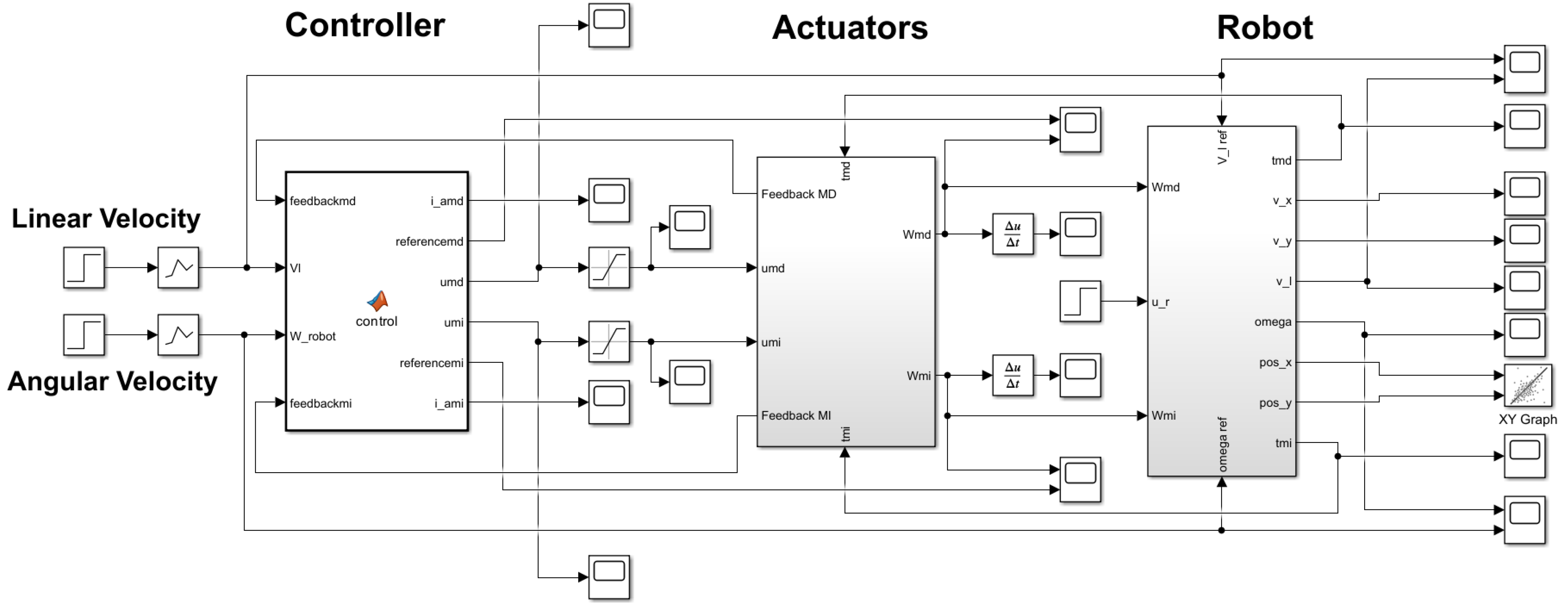
2.2.2. Control System Design

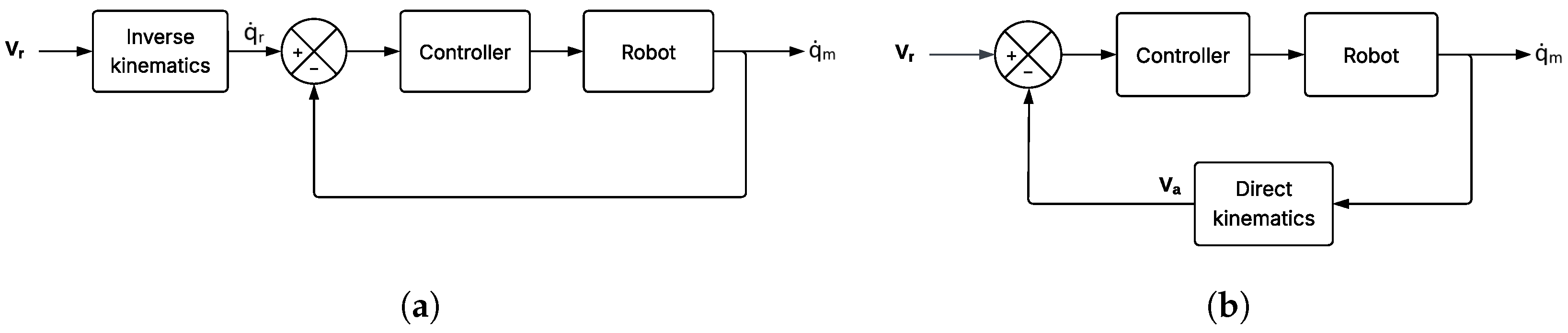
The control system design problem can be approached from two different perspectives, regardless of the controller architecture (PID, state-space controllers, etc.), and the selection of one or the other depends on the available technology. The first approach involves control in the joint (or actuation) space, meaning that the control variables are the individual motor velocities. 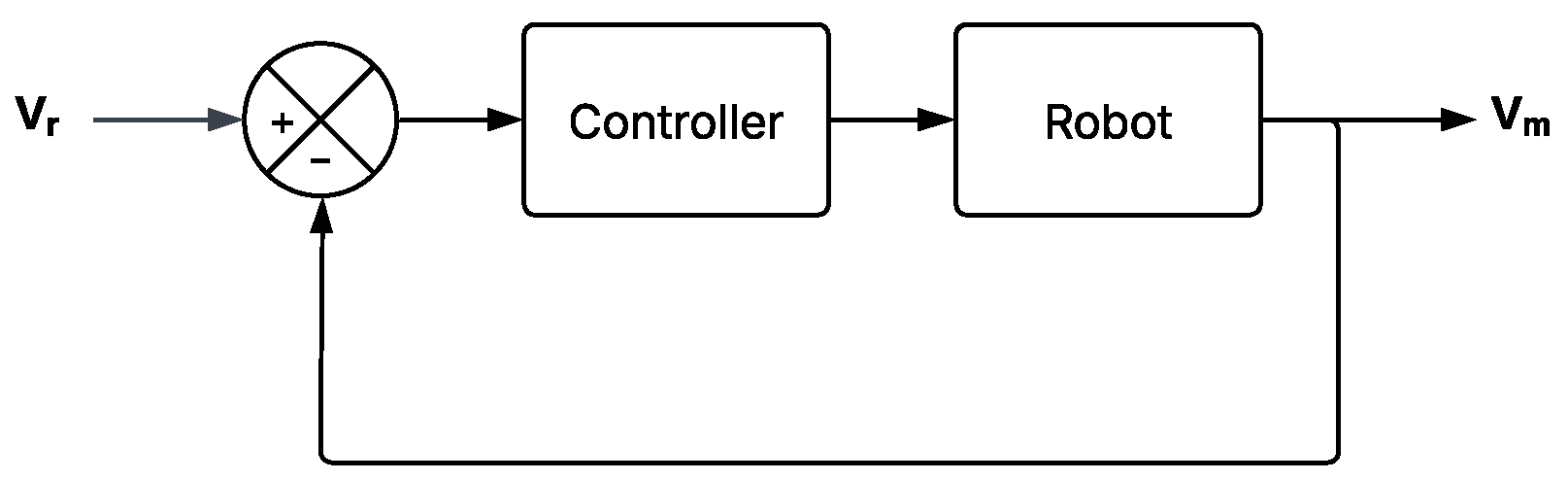This can be implemented in two ways, as illustrated in Figure 10. The second approach consists of control in the workspace, where the control variables are the robot’s linear and angular velocities, as shown in Figure 11.

Figure 10. Robot’s control in the joint space. (a) Control with inverse kinematics. (b) Control with direct kinematics.

Figure 11. Robot control in the workspace.

where

V_r are the reference velocities of the robot (linear and angular).

$\dot{q_r}$ are the reference angular velocities for the motors, calculated using IK.

$\dot{q_m}$ are the angular velocities for each motor measured by the encoders.

V_a are the robot’s velocities, approximated using the motors’ velocities and DK.

V_m are the robot’s measured velocities.

The best option is control in the workspace, as the use of inverse or direct kinematics directly depends on the robot’s parameters, meaning that any change in these parameters must be reflected in the kinematic equations. However, control in the workspace requires sensors that directly measure the linear or angular velocities of the robot. In this study, the only sensors available on the robot were the motor encoders, so the only feasible options were control in the joint space using inverse or direct kinematics. Since the mathematical models of the motors were previously obtained, direct control of the actuators’ angular velocities was the best option, using inverse kinematics.

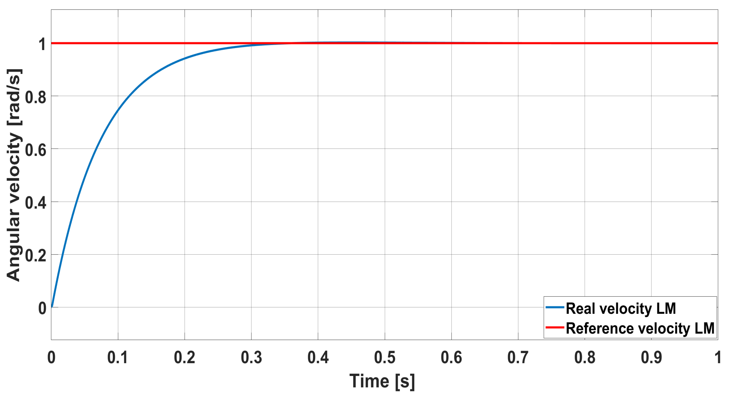
To ensure that the motors’ acceleration did not produce torques greater than previously stated, a response time was proposed that depends on this parameter and the maximum angular velocity.

$$T_s={\displaystyle \frac{{\omega }_{max}}{{\alpha }_{max}}}$$

(19)

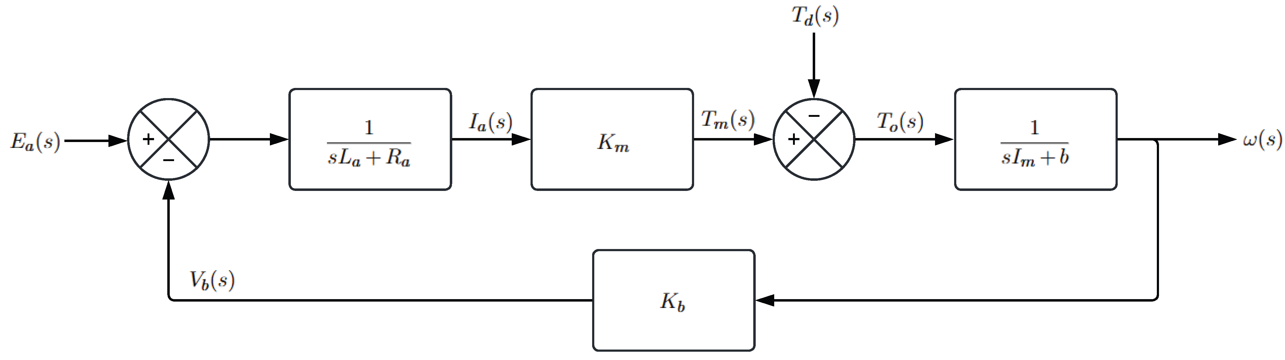
Using Equation (19), a response time of 0.322 s was obtained, indicating that the dominant pole governing the system dynamics must be located at 12.4224. Once the response time had been defined, an additional design criterion was established to ensure zero steady-state error, at least when the reference input exhibits a step-like behavior. Furthermore, the mathematical models of the plants corresponded to underdamped second-order systems, as described by Equation (20).

$$G\left(s\right)={\displaystyle \frac{K·{\omega }_n^2}{s^2+2\zeta {\omega }_{n}s+{\omega }_n^2}}$$

(20)

where

K is the system’s static gain.

${\omega }_n$ is the natural frequency of the system.

$\zeta$ is the damping ratio of the system.

Given the design requirements and the structure of the mathematical model of each system to be controlled, controller options such as PI and PD were discarded. Although a PI controller can achieve zero steady-state error, it lacks the necessary flexibility to shape the time response, as it only introduces one zero, while the plant has two poles. Similarly, a PD controller does not offer sufficient control over the time response for the same reason, and in addition, it cannot ensure a zero steady-state error, due to the absence of a pole at the origin.

On the other hand, classical techniques such as lag, lead, or lag–lead controllers are not suitable options either, since these controllers are essentially “imperfect” versions of integrators or differentiators, which are already present in PI and PD controllers. In the best-case scenario, a lag–lead configuration only approximates the behavior of a full PID controller.

In this context, the viable control strategies for the system included a PID controller, a modern approach based on state-space representation, or an advanced technique such as fuzzy logic or neural networks. The latter two options are typically applied to more complex systems or objectives, such as trajectory tracking or the generation of reference velocities, as discussed in Section 1 and demonstrated in works such as [25,26,27,28,29]. Therefore, for the system considered in this study, the most suitable options were a PID controller or a state-space-based controller.

Of the two options, a PID controller was selected, for the simple reason that a state-space controller requires an observer or estimator to estimate states that cannot be measured in real time (such as the armature current in DC motors). An observer or estimator requires shorter response times, to ensure that the unmeasured states converge before the output response time. Additionally, for the physical implementation discussed in Section 3.3, shorter sampling times are required, even smaller than the response times. While shorter response times improve system performance, the criteria for these times vary in the literature [23,24]. The challenge with shorter response times lies in the encoder resolution of the physical implementation, which provides only 100 samples per revolution. As a result, the sampling time cannot be too short, as this would compromise the reliability of measurements at lower angular velocities of the motors. Thus, the proposal consists of a PID controller, with a transfer function for each motor, as shown in Equation (21).

$$C\left(s\right)={\displaystyle \frac{k_p·{\tau }_d·(s^2+\frac{1}{{\tau }_d}s+\frac{1}{{\tau }_d·{\tau }_i})}{s}}$$

(21)

where

$k_p$ is the proportional gain of the PID controller.

${\tau }_d$ is the derivative time constant.

${\tau }_i$ is the integral time constant.

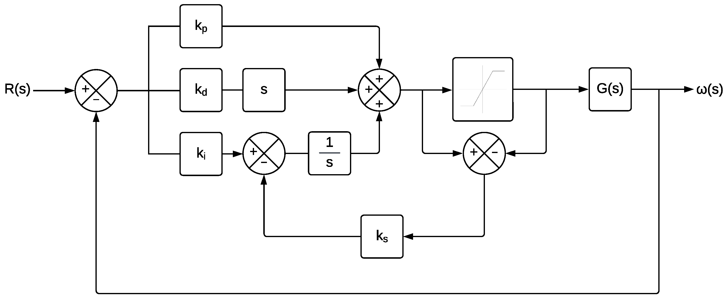
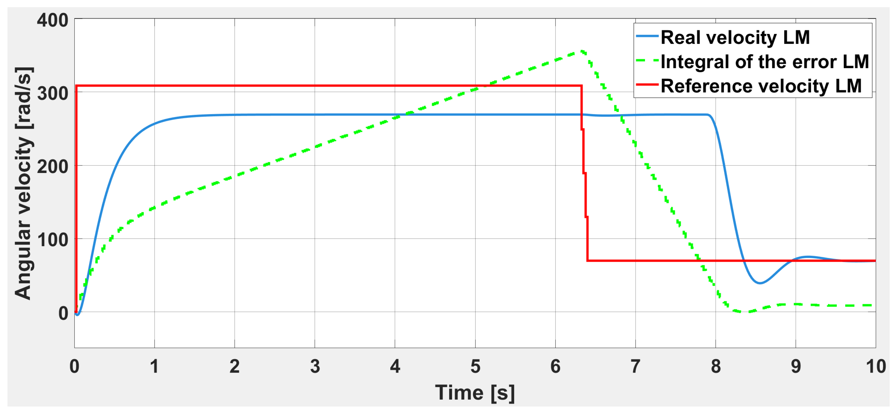
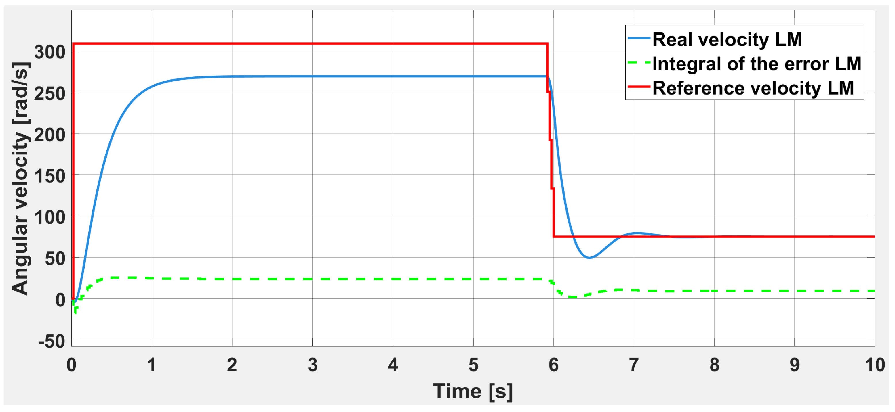
The PID controller is designed in such a way that the dynamics of the plant to be controlled are nullified, ensuring that, in a closed-loop configuration, the system exhibits a first-order transfer function. This is achieved using the pole-zero cancellation method to determine the PID parameters. In this manner, the desired response time can be freely controlled. However, controllers that include an integrative part to eliminate steady-state error have a drawback: when the control signal saturates, which is inevitable in physical systems, the integral of the error starts to accumulate over time, resulting in the windup effect. To mitigate this, it is essential to implement an anti-windup technique, such as those discussed earlier.

Pole-zero cancellation nullifies the plant’s dynamics, ensuring that Equation (22) is satisfied.

$$s^2+2\zeta {\omega }_{n}s+{\omega }_n^2=s^2+{\displaystyle \frac{1}{{\tau }_d}}s+{\displaystyle \frac{1}{{\tau }_d·{\tau }_i}}$$

(22)

In this way, the direct chain of the system is given by Equation (23).

$$C\left(s\right)·G\left(s\right)={\displaystyle \frac{K·{\omega }_n^2·k_p·{\tau }_d}{s}}$$

(23)

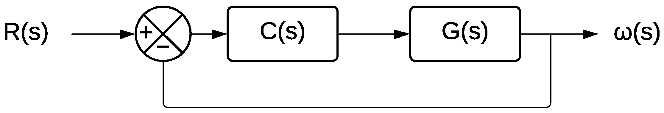
Therefore, considering the unit feedback as shown in the diagram of Figure 12, the closed-loop transfer function is given by Equation (24).

$$T\left(s\right)={\displaystyle \frac{K·{\omega }_n^2·k_p·{\tau }_d}{s+K·{\omega }_n^2·k_p·{\tau }_d}}$$

(24)

Figure 12. Schematic of the control system with unity feedback.

Based on the response time equation for a first-order system, and following the criterion proposed by Nise [23], Equation (25) is obtained.

$$T_s={\displaystyle \frac{4}{K·{\omega }_n^2·k_p·{\tau }_d}}$$

(25)

Equations (22) and (25) allow finding the values of the PID controllers that adjust the response to the desired time and eliminate the steady-state error. These values are shown in Table 5.

Table 5. PID controller parameters for the robot’s motors.

Parameter	Right Motor	Left Motor
kp	0.149347	0.158561
${\tau }_d$	0.067278	0.069166
${\tau }_i$	0.150127	0.158682

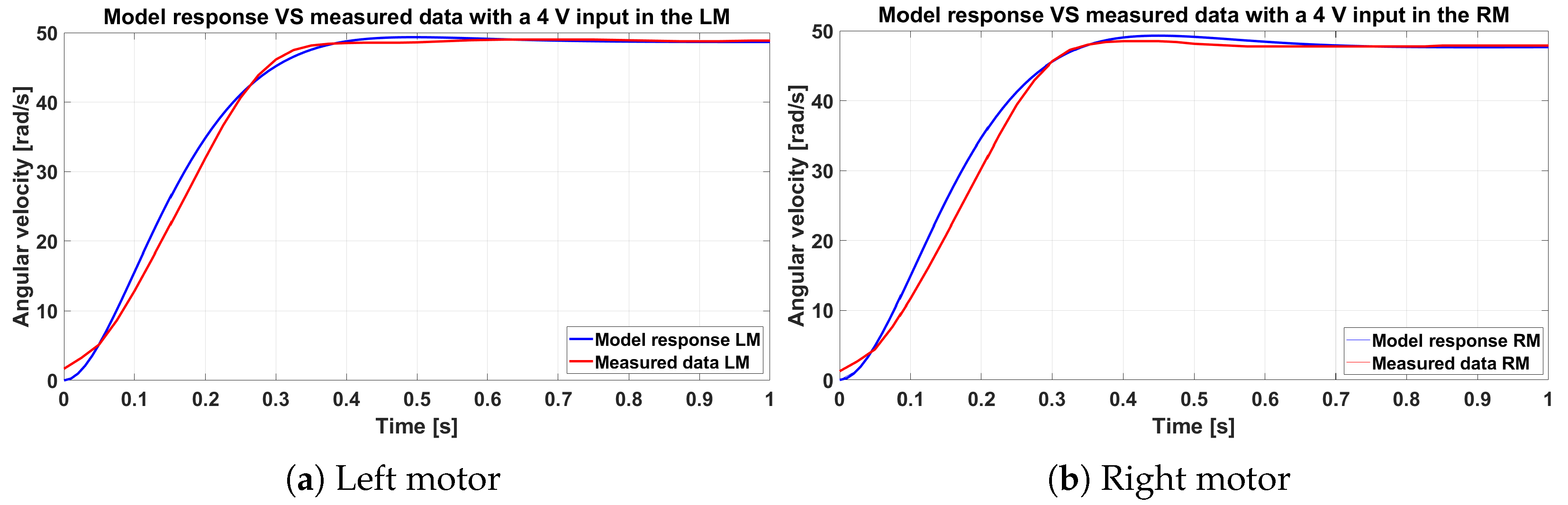
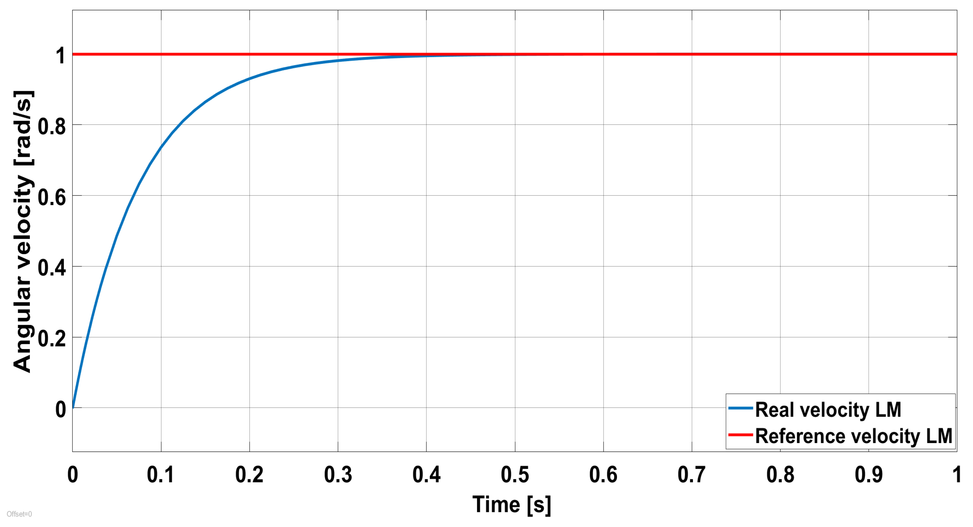
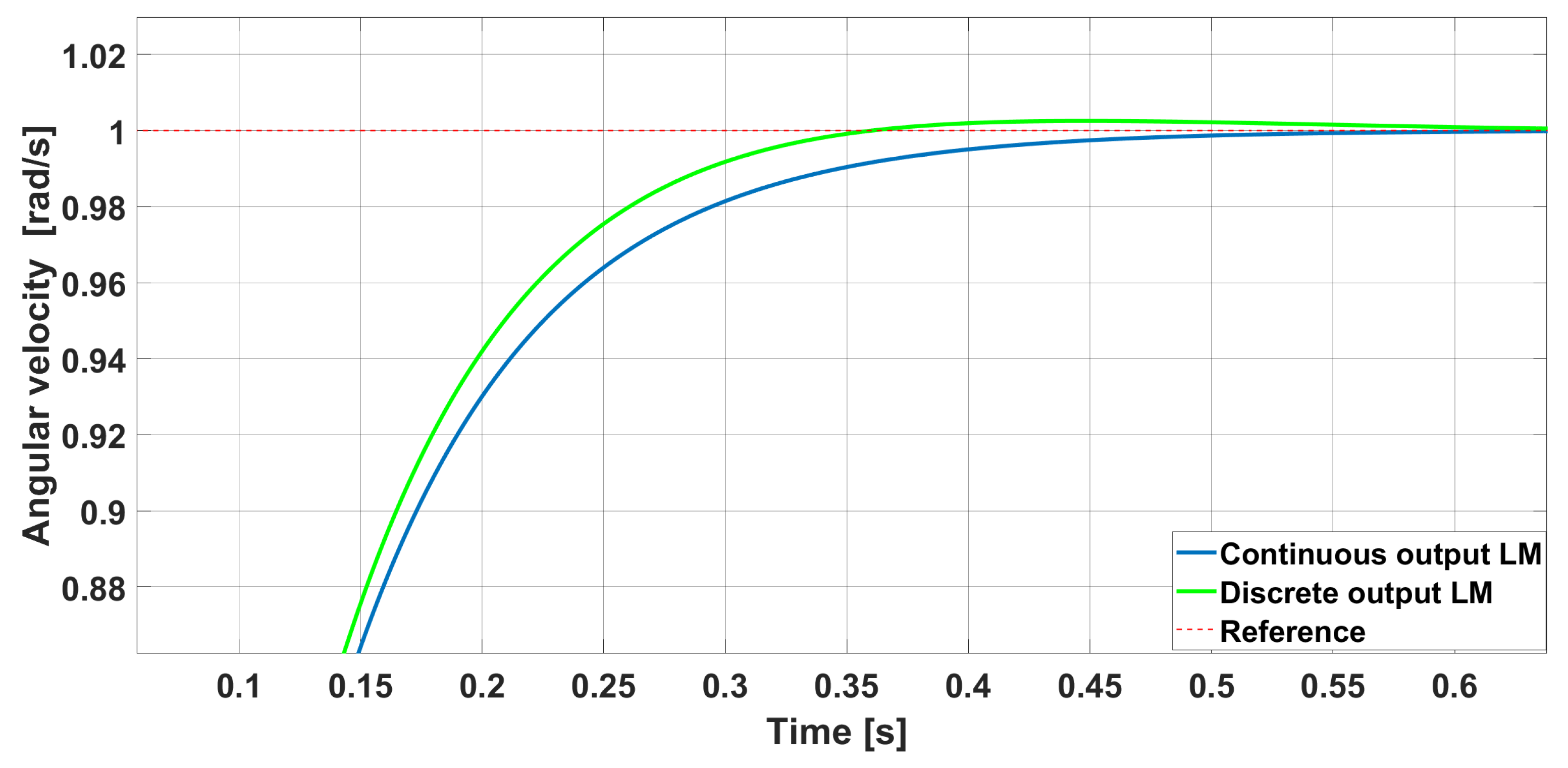
With the controller designed in continuous time, a digital control algorithm can be derived by applying numerical methods to transform the system from the complex domain s to the complex domain z. The complexity of these methods depends on the desired level of precision and accuracy in the approximation; some of the most well-known techniques are discussed in [42]. For the discretization of the controllers, the Backward Euler method was employed, using a sampling time of 25 ms. This value was determined experimentally and corresponds to the minimum interval that ensured accurate measurement of the actual motor velocities.

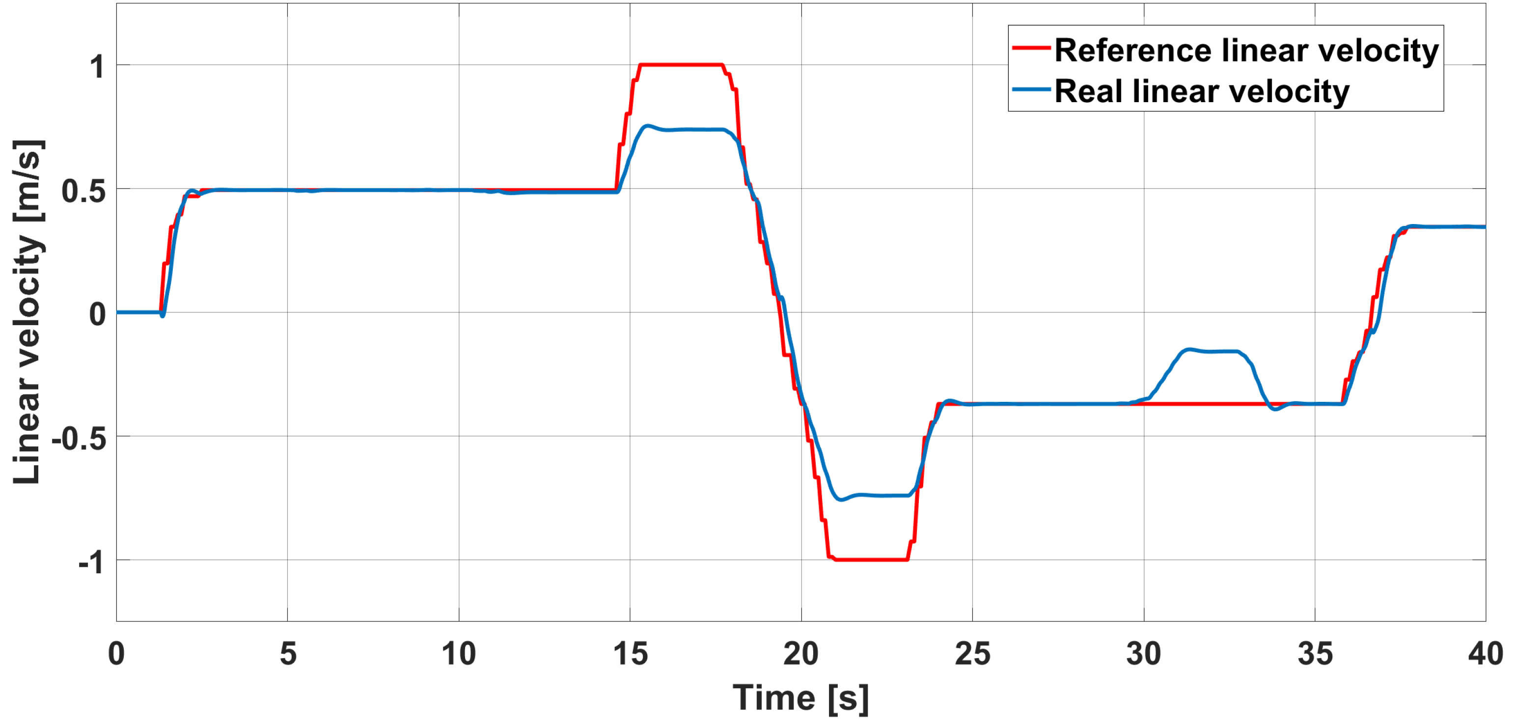
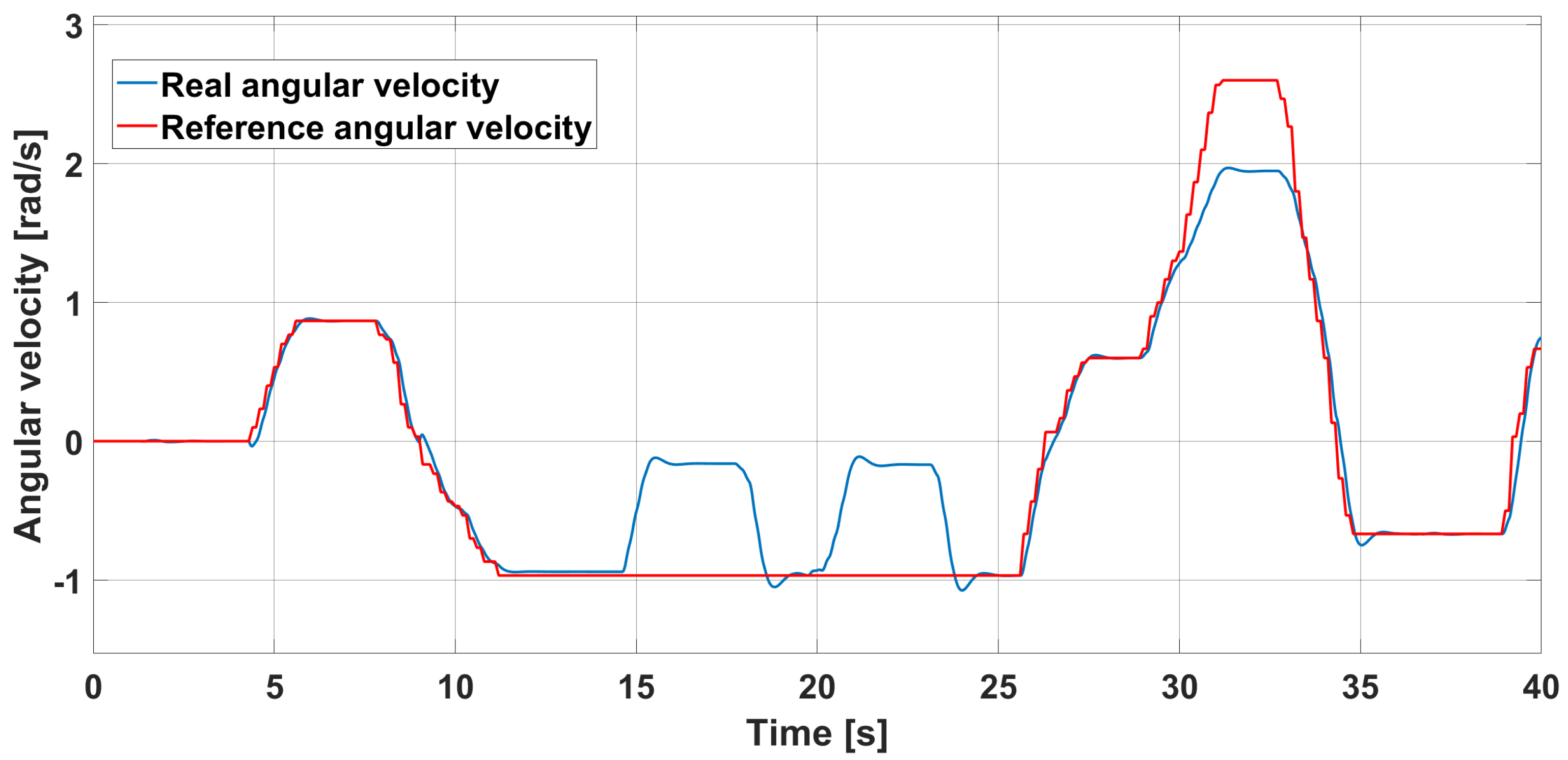
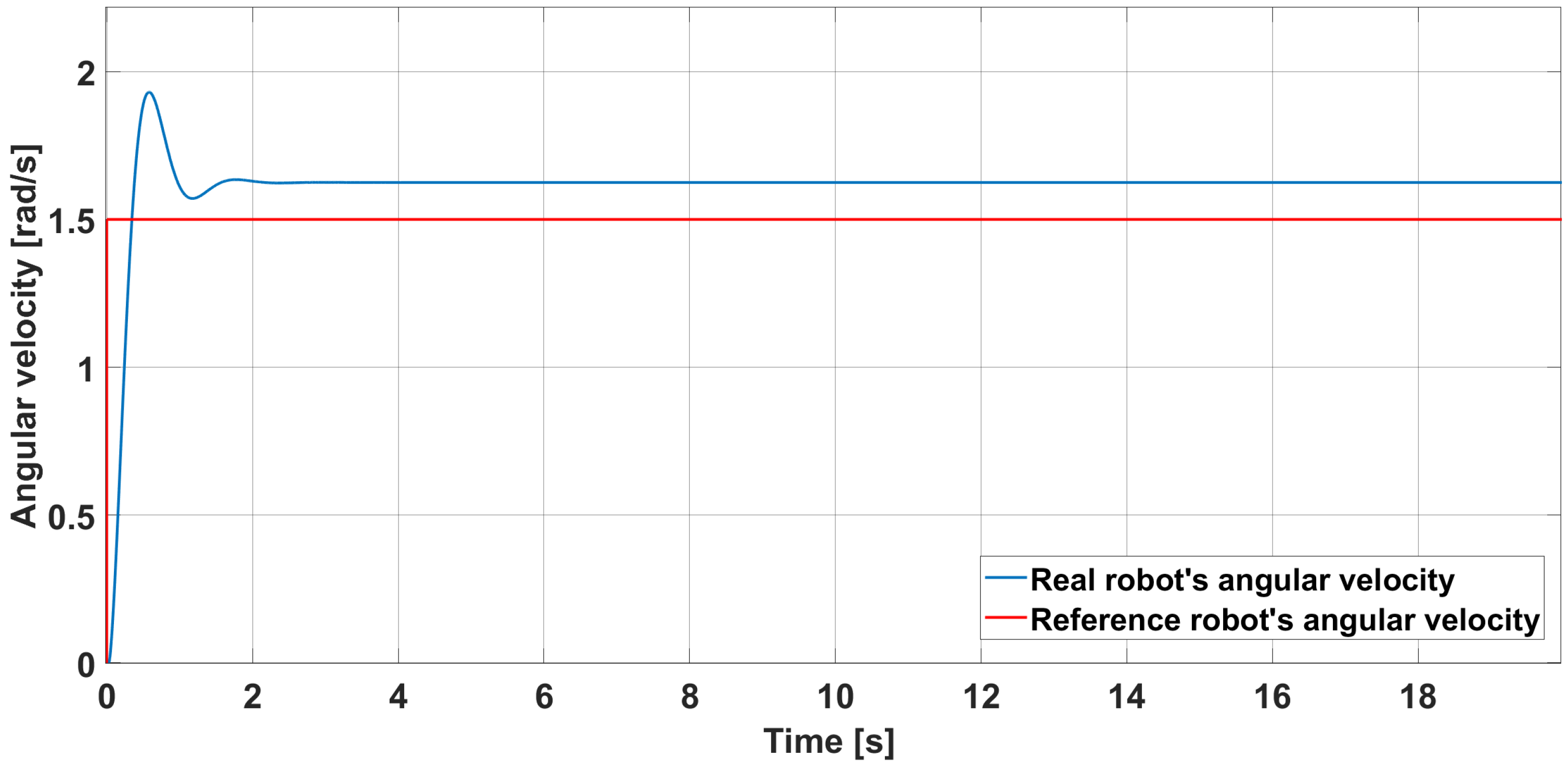
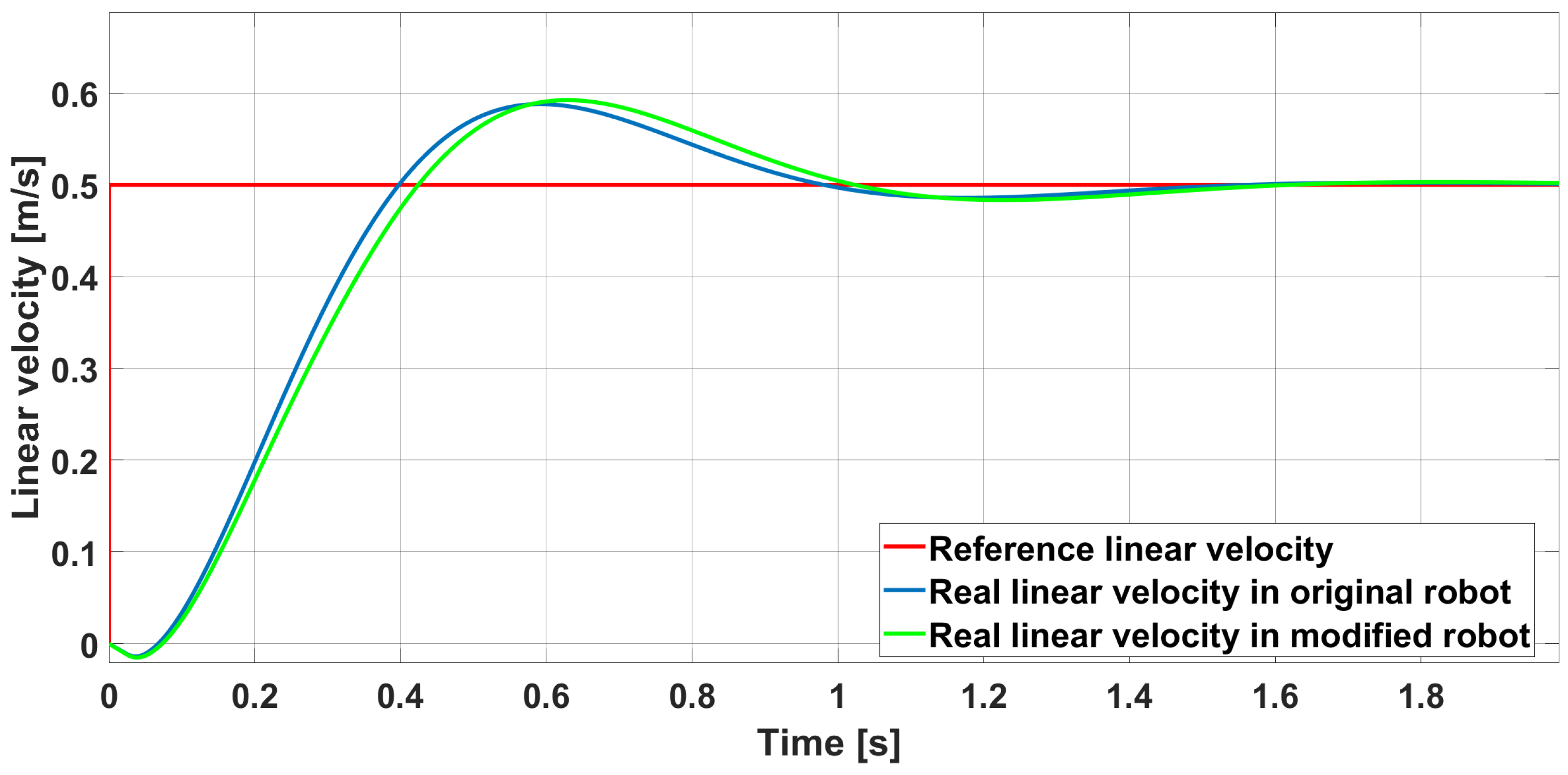
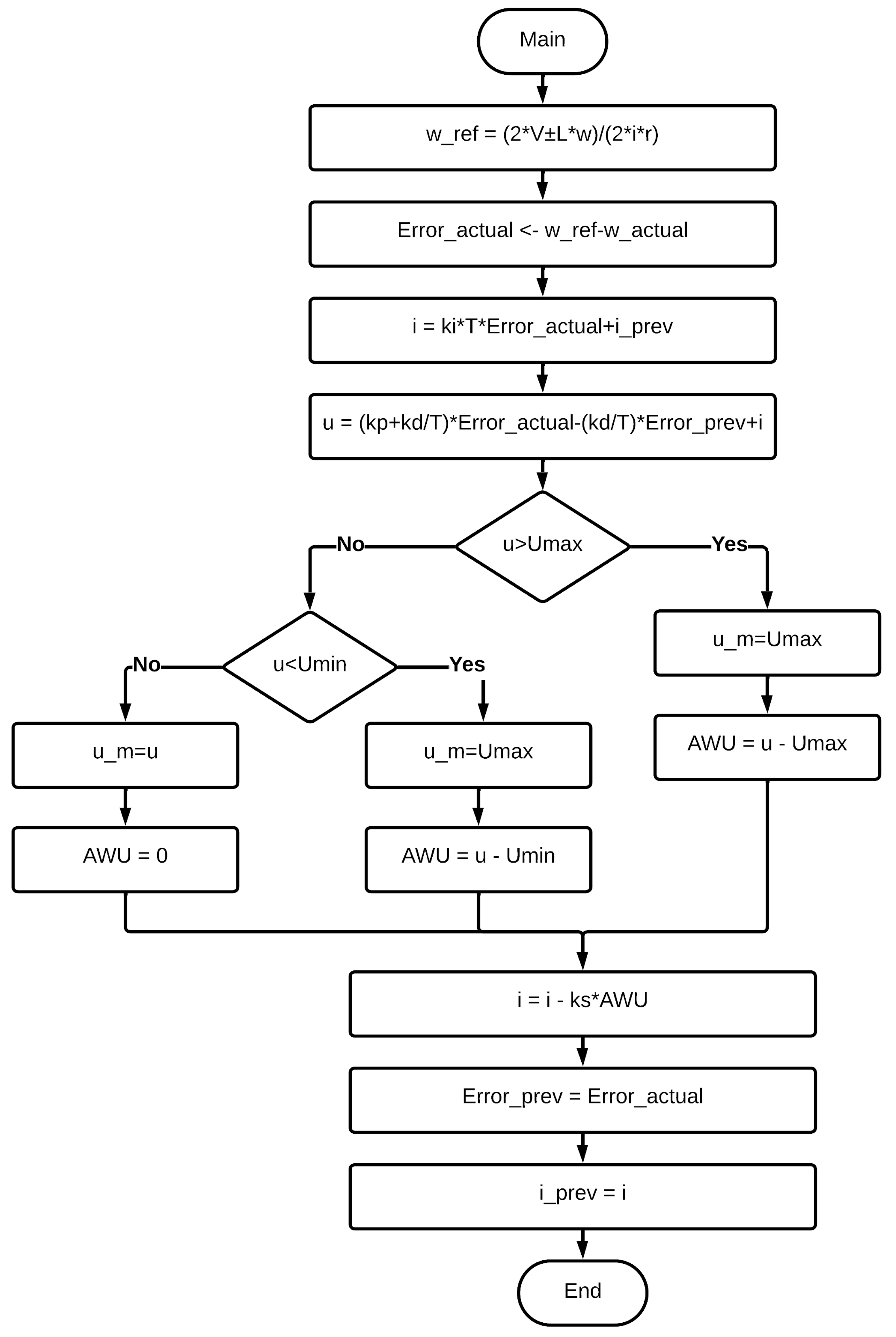
Notably, this sampling time is approximately 13 times shorter than the system’s response time, which ensures a good approximation of the continuous-time behavior, as demonstrated in Section 3.2. If a state-space controller with an observer or estimator had been implemented instead, the response time of the system would have needed to be much shorter, and consequently, the sampling time as well. In this way, the necessary equations for the digital control algorithms were derived with 25 ms for the PID controller, as presented below.

$$u_{RM}\left(k\right)=0.5513·e_{RM}\left(k\right)-0.4019·e_{RM}(k-1)+i_{RM}\left(k\right)$$

(26)

$$i_{RM}\left(k\right)=0.02487·e_{RM}\left(k\right)+i_{RM}(k-1)$$

(27)

$$u_{LM}\left(k\right)=0.5847·e_{LM}\left(k\right)-0.4386·e_{LM}(k-1)+i_{LM}\left(k\right)$$

(28)

$$i_{LM}\left(k\right)=0.0249·e_{LM}\left(k\right)+i_{LM}(k-1)$$

(29)

where

$u_{RM}\left(k\right)$ is the control signal for the right motor in discrete time.

$e_{RM}\left(k\right)$ is the error in the right motor in discrete time.

$i_{RM}\left(k\right)$ is the integral of the error for the right motor in discrete time.

$u_{LM}\left(k\right)$ is the control signal for the left motor in discrete time.

$e_{LM}\left(k\right)$ is the error in the left motor in discrete time.

$i_{LM}\left(k\right)$ is the integral of the error for the left motor in discrete time.

Equations (26) and (28) correspond to the control laws for the right and left motors, respectively, while Equations (27) and (29) correspond to the equations for the error integrals of both motors, in which the anti-windup technique shown in Figure 13 is applied.

Figure 13. Schematic of the control system with unity feedback and anti-windup.

Discretizing the system from Figure 13, the algorithm shown in Figure 14 is obtained.

Figure 14. Schematic of the control system with unity feedback and anti-windup.

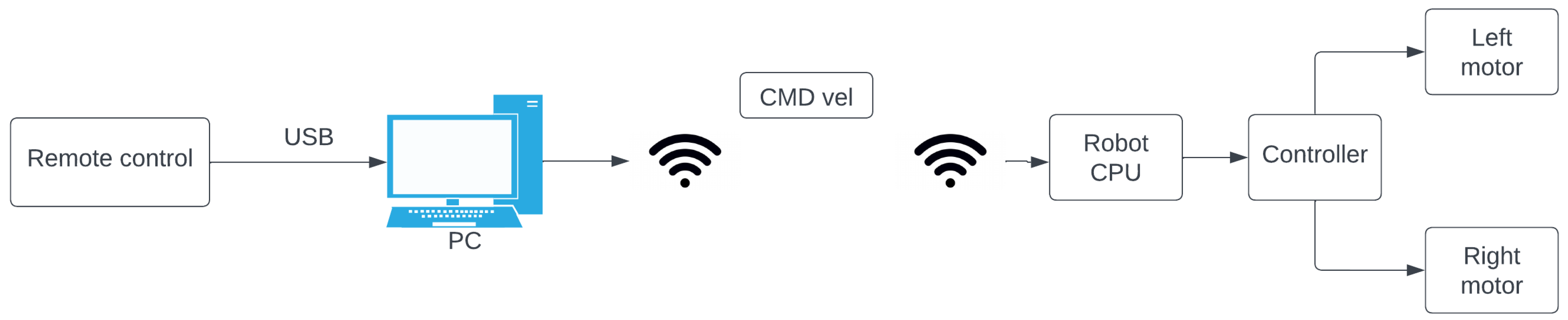
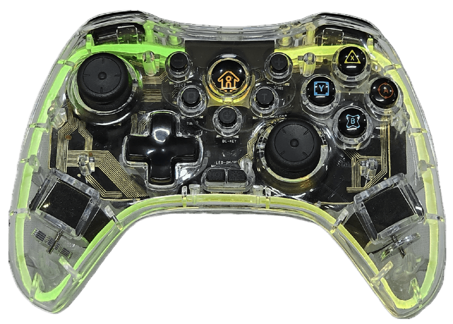
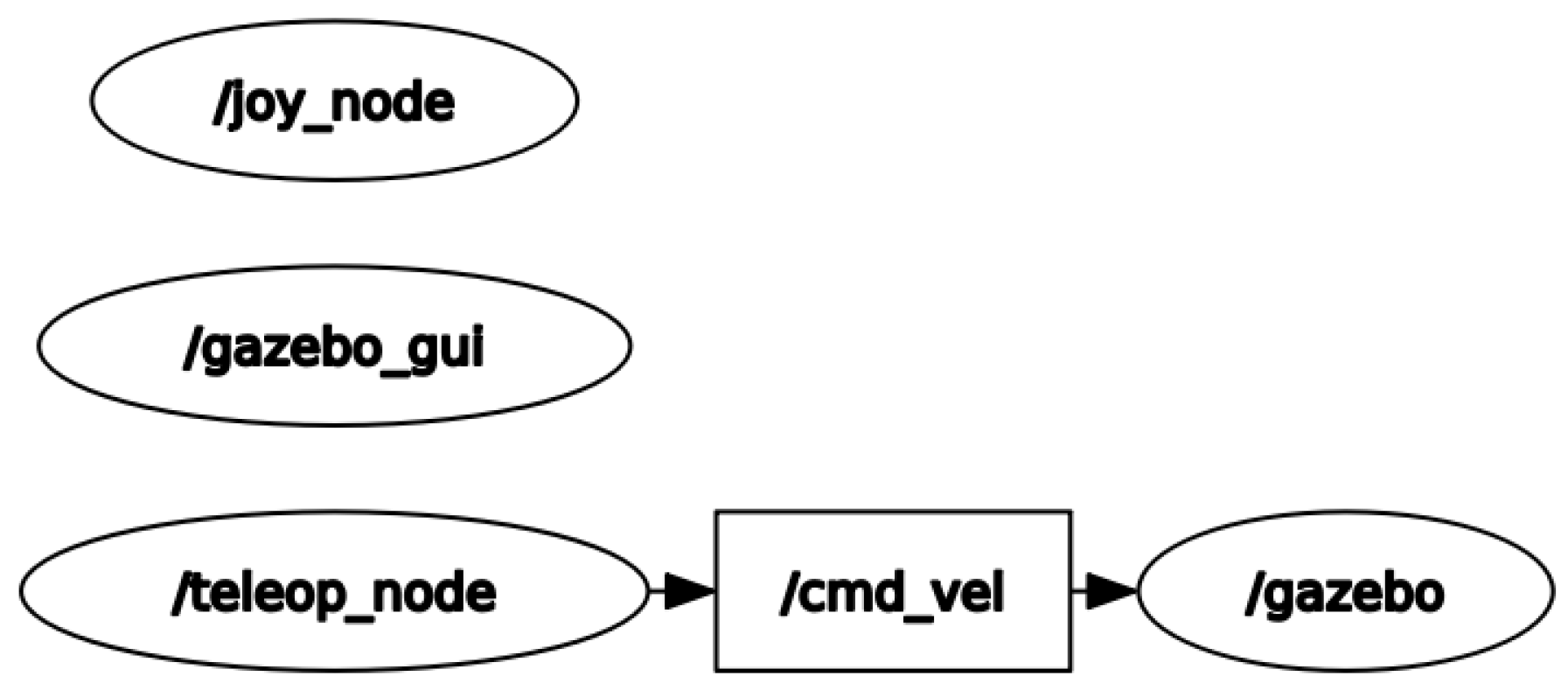
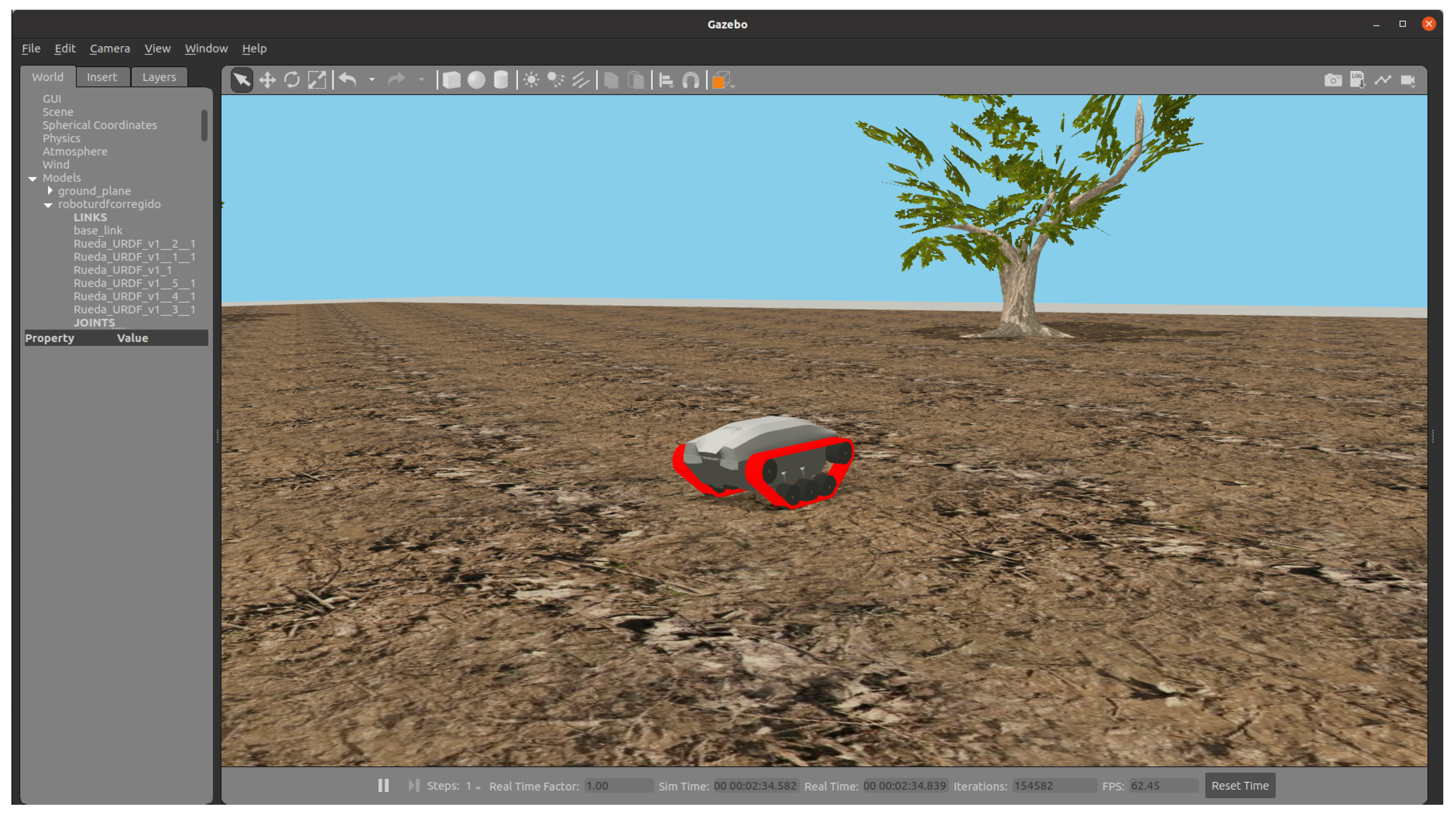
For the physical implementation, the joy_node and teleop_node, shown in Figure 9, were programmed on the master computer. On the other hand, the robot’s CPU received the cmd_vel topic and transmitted these values to the controller via serial communication, maintaining the structure outlined in Figure 7. Based on the robot’s linear and angular velocity values received through the cmd_vel topic, individual references for each motor were calculated using the robot’s kinematic model. These references were subsequently sent to the discretized PID controller, equipped with an anti-windup system to ensure a quick response under saturation conditions.

3. Results

3.1. Implementation of ROS Nodes in Gazebo

The ROS nodes were evaluated through the implementation of a digital twin in Gazebo, using two network-connected computers. The master computer ran the nodes responsible for reading the controller outputs and publishing them as velocity commands, while the slave computer ran the Gazebo node to simulate the robot’s physical movement based on the received velocity data. In this setup, the cmd_vel topic was published by the master and subscribed to by the slave. The digital twin used in this evaluation is illustrated in Figure 15.

Figure 15. Robot digital twin in gazebo environment.

3.2. Simulation of the Control System

Before implementing the control system with the mathematical models of the robot, it was verified that the performance of the controllers tuned using the pole-zero cancellation method met the established design conditions. To achieve this, the control system’s response for both the right motor and the left motor was evaluated in continuous time, obtaining an output curve in response to a step input, as shown in Figure 16.

Figure 16. Performance of the control system for the left motor in response to a step input in continuous time.

The response shape shown in Figure 16 corresponds to the curve of the left motor. However, since the tuning method used for both motors was exactly the same, the right motor’s response exhibited an identical shape. When the control system was discretized and its behavior was analyzed in response to a step input, the resulting curve was as shown in Figure 17.

Figure 17. Performance of the control system for the left motor in response to a step input in discrete time.

Similarly to the previous case, the curve shown in Figure 17 corresponds to the left motor, while the curve for the right motor is practically identical. Additionally, as observed in both figures, the behavior of the two systems was similar, with a slight discrepancy around 0.4 s. At that point, the discrete system deviated from behaving like a first-order system, exhibiting a small overshoot that was negligible. This difference is more clearly seen in Figure 18.

Figure 18. Comparison between the behavior of the continuous and discrete controllers in response to a step input.

The discrepancy between the responses in continuous and discrete time arose because, when discretizing the continuous system, pure integrations and differentiations disappeared. Additionally, the numerical method used for discretization plays a crucial role in determining how well the discrete-time system approximates the continuous-time system.

Another fundamental factor in the discretization of the control system is the sampling time. Regardless of the numerical method used, a shorter sampling interval ensures a better approximation to the continuous-time system. In the case of Figure 18, the discrete-time system demonstrated good performance using the Backward Euler method with a sampling period of 25 ms.

When a saturator was implemented in the previously evaluated control system, the behavior of the response changed dramatically. When the system operated without the anti-windup controller and a saturator, its behavior was as shown in Figure 19. During saturation, when the actuators reached their maximum speed limit, they were unable to precisely track the reference velocity, causing a delay in the system’s response. This delay arose because the controller’s integrative part continued to accumulate error, as the reference was not reached. Once the system returned to its operational limits, the output signal remained unchanged until the integral was fully discharged. It is crucial to note that, even when the control signal is saturated, if the integral continues to grow, the control signal will stay at its saturation limit until the integral is entirely cleared.

Figure 19. Windup effect on the left motor.

To solve this problem, an anti-windup controller was implemented. This controller limits the accumulation of error over time, preventing the error from increasing indefinitely while the system is saturated. Thanks to this controller, when the system exits saturation and returns to its operational limits, the actual velocity adjusts to follow the reference velocity instantaneously, eliminating the delay and improving the system’s response accuracy, as shown in Figure 20. The same controller was applied to the right motor, ensuring the system operated correctly.

Figure 20. Anti-windup effect on the left motor.

As observed in Figure 20, when the system was saturated, it did not reach the desired value, because the control signal could no longer grow to adequately follow the reference. Additionally, this saturation altered the system’s behavior whenever the controller calculated a control signal greater than the saturation limit.

The desired behavior, as shown in Figure 17, will only be achieved if the control signal sent to the actuator always corresponds to the signal calculated by the controller. Otherwise, if saturation persists, even for a short period of time, the desired behavior of a first-order system can be lost. As shown between 6 and 7 s in Figure 20, the system exhibited an underdamped second-order behavior.

Finally, the system was validated using all the mathematical models, aiming to achieve responses as close as possible to those of a physical system. The simulated system is shown in Figure 21.

Figure 21. Mathematical model of the robot implemented in MATLAB/SIMULINK.

The system shown in Figure 21 consists of three fundamental blocks. The first is the controller, which implements the algorithms described in Figure 14 for both motors. Using step inputs for linear and angular velocities, connected to sliders, reference velocities are sent to the robot. Equations (5) and (6) are used to calculate the reference velocities for the motors.

The second block is the actuator, which contains the block diagram shown in Figure 5, where the inputs are the control signal and the disturbance torque. Lastly, the robot block includes kinematic and dynamic models, which allow the generation of graphs showing the linear and angular velocities achieved by the robot. Additionally, the dynamic model provides feedback to the actuators with the load torque generated by the robot.

With the system in operation, the linear velocity graphs, shown in Figure 22, and the angular velocity graphs, shown in Figure 23, were obtained, where the reference velocities are compared with the actual velocities.

Figure 22. Reference linear velocity and linear velocity achieved by the control system.

Figure 23. Reference angular velocity and angular velocity achieved by the control system.

The behavior of the curves in Figure 22 and Figure 23 was due to the saturation or physical limitation of the actuators, which had a maximum angular velocity of 321.6 rad/s. When a combination of linear and angular velocity is presented simultaneously, according to Equations (5) and (6), one of the two motors, depending on the direction of the robot’s movement, will need to exceed its maximum speed to reach the reference values. Since the system cannot achieve this, a steady-state error is generated. Additionally, the load that the motors must overcome reduces their maximum angular velocity, causing the saturation to occur sooner. When the linear velocity is saturated and the reference angular velocity changes, the linear velocity deviates from its reference to try to compensate for the angular velocity; similarly, when the angular velocity is saturated and the linear velocity changes. This effect was evident between 12 and 25 s of the simulation. Likewise, when the system exits saturation and returns to its operational limits, the anti-windup controller allows the output signal to quickly follow the reference, as observed around 35 s.

It is important to clarify that, in this study, there was no way to measure the actual linear and angular velocities directly. However, in Simulink, kinematic models are useful for estimating the real velocities of the robot.

The trajectory obtained using the velocities from Figure 22 and Figure 23 in a 2D plane is shown in Figure 24.

Figure 24. Trajectory obtained in a 2D plane.

As mentioned at the beginning of Section 2.2.2, the direct control of the actuators (control in the joint space) directly depends on the robot’s parameters, especially the geometric parameters used in the direct and inverse kinematics, which are L, r, γ, N₁, and N₂, as shown in Table 1. For example, with the correct parameters, the algorithm in Figure 14 calculated the correct motor velocities, using the inverse kinematics Equations (5) and (6), and the actual velocity followed the reference velocity, as shown in Figure 22 and Figure 23. However, if any robot parameters change and this change is not considered in the control algorithm, the reference tracking will not be accurate. For example, if the L value changes from 0.650048 m to 0.6 m, the tracking velocity behavior will change, as seen in Figure 25.

Figure 25. Robot’s angular velocity with L parameter changed.

According to direct kinematics, in Equations (2) and (3), the L parameter only affects the robot’s angular velocity. Therefore, when this parameter changes, the linear velocity behaves as if there were no change. However, modifications to other previously mentioned parameters affect the tracking of both linear and angular velocities. As a result, the control algorithm cannot correctly estimate and follow the desired velocities if changes in geometric parameters are not considered. This implies that control in the joint space is not reliable when there is uncertainty in the robot’s geometric parameters. Moreover, additional parameters beyond the geometric ones can alter the motor behavior or the robot’s dynamic response. For instance, if the total robot mass changes from 70 kg to 80 kg and the moment of inertia increases from 15.3 kg·m² to 18 kg·m², the reference tracking is affected, as shown in Figure 26.

Figure 26. Robot’s linear velocity with mass and moment of inertia changed.

Note how the real linear velocity of the robot with the original parameters was almost the same as that of the robot with the modified parameters. But why is the system robust in this case and not when a geometric parameter changes? The explanation is simple: the controller can handle variations that do not directly impact the inverse kinematics equations, which are primarily responsible for generating the angular velocity references for both motors. In fact, these references were correctly reached by both the robot with the modified L parameter and the one with the changed mass and moment of inertia. However, in the first case, reaching the angular velocity reference is not enough if the reference itself was miscalculated from the beginning and does not correspond to the desired linear velocity. Therefore, while some uncertainty in the parameters affecting the dynamic model or the motor’s mathematical model can be tolerated due to the controller’s robustness, the geometric parameters used in the kinematic models must be as accurate as possible.

3.3. Implementation of the Navigation System

Once the systems had been validated through simulation, they were physically implemented using a Jetson Nano and an Arduino Mega 2560. At this stage, the control system’s performance was initially evaluated by applying a constant reference value for linear velocity, followed by a constant reference value for angular velocity. The results obtained demonstrated that the system’s responses met the established requirements. Figure 27 shows the graphs of the reference signal and the measured signal for linear velocity, while Figure 28 presents the corresponding graphs for angular velocity.

Figure 27. Reference linear velocity and linear velocity achieved by the control system.

Figure 28. Reference angular velocity and angular velocity achieved by the control system.

It is important to clarify that all tests were conducted using only the motors, with the objective of validating the navigation system, at least without any load on the motors. This is because the robot’s structure and transmission system are still under construction. Therefore, in this subsection, only the verification of the correct operation of the control system and the programmed ROS nodes was carried out, ensuring that the motors achieved the velocities commanded by the joysticks. The data collected from the control system evaluation, shown in Figure 27 and Figure 28, were gathered by the encoders and transmitted to the control loop in the Arduino. These data were obtained using the Arduino plotter.

The horizontal axis of both graphs indicates the number of samples taken at regular intervals of 25 milliseconds, corresponding to the sampling time. This means that every 100 samples represent a 2.5 s interval. It can be observed that the process signal reached the reference value around sample 15, which was approximately 0.375 s. Furthermore, as shown in the figures, the steady-state error was zero, demonstrating the correct performance of the system.

With the control system operating correctly, the master computer nodes were activated, and the serial connection between the Arduino and the Jetson Nano was established. From the Arduino code, the most relevant data were published on a new topic named w_m, which maintained the same structure as the cmd_vel topic. In this topic, the components x, y and z correspond to the control signal, the reference motor velocity, and the measured motor velocity, respectively. It is important to highlight that the linear velocity components are associated with the left motor, while the angular velocity components correspond to the right motor. These data were displayed using the Ubuntu terminal on the robot’s PC (Jetson Nano) and shown on a screen. This structure allowed the values presented in Table 6 and Table 7 to be obtained from two samples.

Table 6. Topic w_m with the most relevant data from the control system of the right motor.

Parameter	Sample 1	Sample 2
Control signal	24	23.329802
Reference velocity	321.781036	321.781036
Real velocity	314.335205	316.823334

Table 7. Topic w_m with the most relevant data from the control system of the left motor.

Parameter	Sample 1	Sample 2
Control signal	24	22.253660
Reference velocity	321.781036	321.781036
Real velocity	316.823334	319.726166

As shown in Figure 27 and Figure 28, the measured signal had some noise due to the sensor, which caused the variations observed in the control signal and the actual measured velocity, as shown in Table 6 and Table 7.

4. Conclusions

The acquisition of robot parameters from mathematical models, datasheets, and mechanical design specifications is a crucial aspect, as these serve as input variables for designing a navigation system. In this work, three main stages were addressed: programming the ROS, controller design, and physical implementation. Programming the robot using the ROS enabled the networking of a digital twin of the robot simulated on a computer, with another computer used to control the system’s navigation via a remote control with joysticks.

On the other hand, the selected PID controller met all the established requirements, demonstrating optimal performance in the system simulated in MATLAB/SIMULINK R2024b. In this simulation, the most relevant parameters were considered to make the system resemble a real system as closely as possible, taking into account physical limitations such as the operational range of the actuators. To address these constraints, solutions such as the anti-windup compensator were proposed, designed to prevent excessive error accumulation.

Finally, the physical implementation of the navigation system allowed the validation of both the performance of the programmed nodes and the designed control system. These components were seamlessly integrated with the physical equipment that will operate the robot, demonstrating the proper functioning of its remote navigation.

References

- Baturone, A. Introducción a la robótica. In Robótica: Manipuladores y Robots Móviles; Marcombo: Barcelona, Spain, 2005; p. 1. [Google Scholar]
- Raj, R.; Kos, A. A Comprehensive Study of Mobile Robot: History, Developments, Applications, and Future Research Perspectives. Appl. Sci. 2022, 12, 6951. [Google Scholar] [CrossRef]
- Valencia, J.A.; Montoya, A.; Rios, L.H. Modelo cinemático de un robot móvil tipo diferencial y navegación a partir de la estimación odométrica. Sci. Tech. 2009, 1, 191–196. [Google Scholar]
- Feng, S.; Liu, Y.; Pressgrove, I.; Ben-Tzvi, P. Autonomous Alignment and Docking Control for a Self-Reconfigurable Modular Mobile Robotic System. Robotics 2024, 13, 81. [Google Scholar] [CrossRef]
- Chen, X.; Jia, Y.; Matsuno, F. Tracking control for differential-drive mobile robots with diamond-shaped input constraints. IEEE Trans. Control Syst. Technol. 2014, 22, 1999–2006. [Google Scholar] [CrossRef]
- Giorgi, C.D.; Palma, D.D.; Parlangeli, G. Online Odometry Calibration for Differential Drive Mobile Robots in Low Traction Conditions with Slippage. Robotics 2024, 13, 7. [Google Scholar] [CrossRef]
- Kouvakas, N.D.; Koumboulis, F.N.; Sigalas, J. A Two Stage Nonlinear I/O Decoupling and Partially Wireless Controller for Differential Drive Mobile Robots. Robotics 2024, 13, 26. [Google Scholar] [CrossRef]
- He, S. Feedback control design of differential-drive wheeled mobile robots. In Proceedings of the ICAR ’05 Proceedings, 12th International Conference on Advanced Robotics, Seattle, WA, USA, 18–20 July 2005; pp. 135–140. [Google Scholar] [CrossRef]
- Sotelo Gomez, A.A. Implementación de un Robot Explorador con Realidad Virtual para Incrementar la Seguridad de la Institución Educativa 7213 Peruano Japonés en el Distrito de Villa el Salvador–2020. Bachelor’s Thesis, Universidad Privada del Norte, Trujillo, Peru, 2020. [Google Scholar]
- Martinez, J.; Mandow, A.; Morales, J.; Garcia-Cerezo, A.; Pedraza, S. Kinematic modelling of tracked vehicles by experimental identification. In Proceedings of the 2004 IEEE/RSJ International Conference on Intelligent Robots and Systems (IROS) (IEEE Cat. No. 04CH37566), Sendai, Japan, 28 September–2 October 2004; Volume 2, pp. 1487–1492. [Google Scholar] [CrossRef]
- Moosavian, S.A.A.; Kalantari, A. Experimental Slip Estimation for Exact Kinematics Modelling and Control of a Tracked Mobile Robot. In Proceedings of the 2008 IEEE/RSJ International Conference on Intelligent Robots and Systems, Nice, France, 22–26 September 2008. [Google Scholar] [CrossRef]
- Iossaqui, J.G.; Camino, J.F.; Zampieri, D.E. A nonlinear control design for tracked robots with longitudinal slip. IFAC Proc. Vol. 2011, 44, 5932–5937. [Google Scholar] [CrossRef]
- Choset, H.; Lynch, K.M.; Hutchinson, S.; Kantor, G.A.; Burgard, W. Configuration Space. In Principles of Robot Motion: Theory, Algorithms, and Implementations; MIT Press: Cambridge, MA, USA, 2005; pp. 47–68. [Google Scholar]
- Spong, M.W.; Hutchinson, S.; Vidyasagar, M. Dymamics and motion planning. In Robot Modeling and Control, 2nd ed.; John Wiley & Sons: Hoboken, NJ, USA, 2020; Volume 1, pp. 165–214. [Google Scholar]
- Du, K.L.; Swamy, M.N.S. Wireless Communication Systems. In Proceedings of the Conference Record of 2004 Annual Pulp and Paper Industry Technical Conference (IEEE Cat. No.04CH37523), Victoria, BC, Canada, 27 June–1 July 2004; Cambridge University Press: Cambridge, UK, 2010; pp. 94–101. [Google Scholar] [CrossRef]
- Blanco Abia, C. Desarrollo de un Sistema de Navegación Para un Robot Móvil. Ph.D. Thesis, Universidad de Valladolid, Escuela de Ingenierías Industriales, Valladolid, Spain, 2014. [Google Scholar]
- Nasirian, A.; Khanesar, M.A.-P. Sliding mode fuzzy rule base bilateral teleoperation control of 2-DOF SCARA system. In Proceedings of the 2016 International Conference on Automatic Control and Dynamic Optimization Techniques (ICACDOT), Pune, India, 9–10 September 2016; pp. 7–12. [Google Scholar] [CrossRef]
- González A., H.; Mejía Castañeda, C.A. Estudio comparativo de tres técnicas de navegación para robots móviles. Rev. UIS Ing. 2007, 6, 77–84. [Google Scholar]
- Chapman, S. Motores y generadores de corriente directa. In Máquinas Eléctricas, 5th ed.; Mc Graw Hill: Columbus, OH, USA, 2012; pp. 345–413. [Google Scholar]
- Nise, N.S. Modeling in the frequency domain. In Control Systems Engineering, 8th ed.; John Wiley & Sons: Hoboken, NJ, USA, 2020; pp. 33–115. [Google Scholar]
- Stefek, A.; van Pham, T.; Krivanek, V.; Pham, K.L. Energy comparison of controllers used for a differential drive wheeled mobile robot. IEEE Access 2020, 8, 170915–170927. [Google Scholar] [CrossRef]
- Rahayu, E.S.; Ma’arif, A.; Cakan, A. Particle Swarm Optimization (PSO) Tuning of PID Control on DC Motor. Int. J. Robot. Control Syst. 2022, 2, 435–447. [Google Scholar] [CrossRef]
- Nise, N.S. Controller Design. In Control Systems Engineering, 8th ed.; John Wiley & Sons: Hoboken, NJ, USA, 2020; pp. 455–721. [Google Scholar]
- Ogata, K. Diseño de controladores. In Ingeniería de Control Moderna, 5th ed.; Pearson Educación: Madrid, Spain, 2010; pp. 416–745. [Google Scholar]
- Lee, C. Fuzzy logic in control systems: Fuzzy logic controller. I. IEEE Trans. Syst. Man Cybern. 1990, 20, 404–418. [Google Scholar] [CrossRef]
- Sierra-García, J.E.; Santos, M. Redes neuronales y aprendizaje por refuerzo en el control de turbinas eólicas. Rev. Iberoam. Autom. Inform. Ind. 2021, 18, 327–335. [Google Scholar] [CrossRef]
- Tolossa, T.D.; Gunasekaran, M.; Halder, K.; Verma, H.K.; Parswal, S.S.; Jorwal, N.; Joseph, F.O.M.; Hote, Y.V. Trajectory tracking control of a mobile robot using fuzzy logic controller with optimal parameters. Robotica 2024, 42, 2801–2824. [Google Scholar] [CrossRef]
- Stavrinidis, S.; Zacharia, P.; Xidias, E. A Fuzzy Control Strategy for Multi-Goal Autonomous Robot Navigation. Sensors 2025, 25, 446. [Google Scholar] [CrossRef]
- Stavrinidis, S.; Zacharia, P. An ANFIS-Based Strategy for Autonomous Robot Collision-Free Navigation in Dynamic Environments. Robotics 2024, 13, 124. [Google Scholar] [CrossRef]
- Carlucho, I.; Paula, M.D.; Acosta, G.G. Double Q-PID algorithm for mobile robot control. Expert Syst. Appl. 2019, 137, 292–307. [Google Scholar] [CrossRef]
- Bârsan, A. Position Control of a Mobile Robot through PID Controller. Acta Univ. Cibiniensis. Tech. Ser. 2019, 71, 14–20. [Google Scholar] [CrossRef]
- Padhy, P.K.; Sasaki, T.; Nakamura, S.; Hashimoto, H. Modeling and position control of mobile robot. In Proceedings of the 2010 11th IEEE International Workshop on Advanced Motion Control (AMC), Nagaoka, Japan, 21–24 March 2010; pp. 100–105. [Google Scholar] [CrossRef]
- Sajnekar, D.M.; Deshpande, S.B.; Mohril, R.M. Comparison of Pole Placement & Pole Zero Cancellation Method for Tuning PID Controller of A Digital Excitation Control System. Int. J. Sci. Res. Publ. 2013, 3, 1–7. [Google Scholar]
- Kim, K.; Schaefer, R. Tuning a PID controller for a digital excitation control system. In Proceedings of the Conference Record of 2004 Annual Pulp and Paper Industry Technical Conference (IEEE Cat. No.04CH37523), Victoria, BC, Canada, 27 June–1 July 2004; pp. 94–101. [Google Scholar] [CrossRef]
- Zhang, W.; Cui, Y.; Ding, X. An improved analytical tuning rule of a robust pid controller for integrating systems with time delay based on the multiple dominant pole-placement method. Symmetry 2020, 12, 1449. [Google Scholar] [CrossRef]
- Peng, Y.; Vrancic, D.; Hanus, R. Anti-windup, bumpless, and conditioned transfer techniques for PID controllers. IEEE Control Syst. 1996, 16, 48–57. [Google Scholar] [CrossRef]
- Bohn, C.; Atherton, D.P. An analysis package comparing PID anti-windup strategies. IEEE Control Syst. 1995, 15, 34–40. [Google Scholar] [CrossRef]
- Gün, A. Attitude control of a quadrotor using PID controller based on differential evolution algorithm. Expert Syst. Appl. 2023, 229, 120518. [Google Scholar] [CrossRef]
- Mousakazemi, S.M.H.; Ayoobian, N. Robust tuned PID controller with PSO based on two-point kinetic model and adaptive disturbance rejection for a PWR-type reactor. Prog. Nucl. Energy 2019, 111, 183–194. [Google Scholar] [CrossRef]
- Mosaad, A.M.; Attia, M.A.-P.; Abdelaziz, A.Y. Whale optimization algorithm to tune PID and PIDA controllers on AVR system. Ain Shams Eng. J. 2019, 10, 755–767. [Google Scholar] [CrossRef]
- Jia, W.; Liu, X.; Jia, G.; Zhang, C.; Sun, B. Research on the Prediction Model of Engine Output Torque and Real-Time Estimation of the Road Rolling Resistance Coefficient in Tracked Vehicles. Sensors 2023, 23, 7549. [Google Scholar] [CrossRef]
- FunctionBay, Inc. Discrete Time Integrator, n.d. Available online: https://functionbay.com/documentation/onlinehelp/default.htm#!Documents/discretetimeintegrator.htm (accessed on 10 July 2024).
Disclaimer/Publisher’s Note: The statements, opinions and data contained in all publications are solely those of the individual author(s) and contributor(s) and not of MDPI and/or the editor(s). MDPI and/or the editor(s) disclaim responsibility for any injury to people or property resulting from any ideas, methods, instructions or products referred to in the content. |
© 2025 by the authors. Licensee MDPI, Basel, Switzerland. This article is an open access article distributed under the terms and conditions of the Creative Commons Attribution (CC BY) license (https://creativecommons.org/licenses/by/4.0/).