Research on Pavement Crack Detection Based on Random Structure Forest and Density Clustering

Abstract

The automatic detection of road surface cracks is a crucial task in road maintenance, but the complexity of crack topology and the susceptibility of detection results to environmental interference make it challenging. To address this issue, this paper proposes an automatic crack detection method based on density clustering using random forest. First, a shadow elimination method based on brightness division is proposed to address the issue of lighting conditions affecting detection results in road images. This method compensates for brightness and enhances details, eliminating shadows while preserving texture information. Second, by combining the random forest algorithm with density clustering, the impact of noise on crack extraction is reduced, enabling the complete extraction and screening of crack information. This overcomes the shortcomings of the random forest method, which only detects crack edge information with low accuracy. The algorithm proposed in this paper was tested on the CFD and Cracktree200 datasets, achieving precision of 87.4% and 84.6%, recall rates of 83.9% and 82.6%, and F-1 scores of 85.6% and 83.6%, respectively. Compared to the CrackForest algorithm, it significantly improves accuracy, recall rate, and F-1 score. Compared to the UNet++ and Deeplabv3+ algorithms, it also achieves better detection results. The results show that the algorithm proposed in this paper can effectively overcome the impact of uneven brightness and complex topological structures on crack target detection, improving the accuracy of road crack detection and surpassing similar algorithms. It can provide technical support for the automatic detection of road surface cracks.

1. Introduction

Cracks, as one of the most common and harmful distresses on road surfaces, are important reference indicators for evaluating road conditions in terms of their quantity, length, and width. The existence of cracks can cause discontinuity in the road surface, reduce the load transmission capacity of the entire road structure, seriously affect the normal operation of the road system, and endanger driving safety [1]. Traditional visual crack detection inevitably leads to waste of time and manpower, low accuracy and efficiency, and is prone to errors. With the rapid development of computer and digital graphics processing technology, the design of practical and effective automatic detection methods for road cracks has sparked discussions among many researchers [2,3,4,5].

Road crack detection is often based on traditional crack detection methods such as image segmentation [6,7,8], image edge detection [9,10], and image enhancement [11,12]. These algorithms classify crack pixels from the background by calculating thresholds for the entire image or its segments. These algorithms can accurately detect cracks in high-contrast images, but when affected by noise such as oil stains and shadows, they may misinterpret noise as cracks, leading to significant false positives and missed detections [13].

Many researchers are also committed to road noise removal algorithms. The methods for removing road surface shadows and other noise can be roughly divided into two types: automated shadow removal methods and interactive shadow removal methods. The fundamental difference between the two lies in how to perform the initial detection of shadows, each with its own advantages and disadvantages. Chua et al. [14] detected road surface shadows based on the edge features of shadows (changes in intensity, texture, and color ratio). Landabaso et al. [15] used morphological reconstruction to remove shadows. Gong Han et al. [16] applied a curve fitting model to improve the quality of intensity sampling for lighting estimation through an intelligent sampling scheme, assuming that the constraint curve or surface function of lighting changes is height limited, while also limiting their range of movable shadows. Khar et al. [17] applied a Bayesian formula to remove common road surface shadows, which contains a large number of unknown parameters and has a high computational complexity, resulting in long computation time and inability to handle shadows in complex scenes. Some recent methods, like differential correction [18] and generative adversarial networks (GANs) [19], detect and remove shadows more effectively. However, these two methods are more complex. The above algorithms have indeed reduced noise-related errors to some extent, but they struggle with noise in complex topologies.

In recent years, automatic monitoring methods for road cracks using machine learning and deep learning have emerged [20,21,22]. There are many deep learning methods for automatic recognition of road cracks, including faster region convolutional neural networks (Faster R-CNN [23,24]), mask region neural networks (Mask R-CNN [25,26]), neural networks (CNN) [27], deep clustering algorithms based on CAE pre training (DCEC) [28], UNet [29], Deeplab [30], etc., which have been applied to road crack detection and have achieved good detection results. The issues of misjudgment and missed detections have also been greatly improved. However, deep learning algorithm models contain a large number of parameters and require a large amount of data training sets. The high cost of manually annotating data makes it difficult to implement deep learning algorithms.

Structured output learning is another important supervised method for road crack detection [31]. Nowozin and Sebastian [32] proposed structured learning methods and introduced popular structured models in computer vision. Kontschieder et al. [33] proposed a simple and effective method for integrating random forest structure information, which expands the random forest with structured label information and applies it to semantic image labeling problems. Dollar and Zitnick [34] proposed a generalized structured learning method for edge detection, which maps structured labels to a discrete space and calculates information gain in the discrete space, thereby reducing the time complexity of the algorithm. On this basis, Yong Shi et al. [31] proposed a road crack detection method based on random structured forest (called CrackForest). The CrackForest model characterizes cracks through two statistical histograms and utilizes algorithms such as support vector machine (SVM) and k-means clustering to distinguish cracks from noise, resulting in preliminary detection outcomes. The CrackForest model has two main shortcomings: it performs poorly on images with significant gradient changes due to interference from oil pollution and shadows. Secondly, as the CrackForest model is essentially an edge detection model, the initial detection results obtained by the model only contain the edge information of cracks. To detect complete cracks, morphological operations like erosion and dilation are performed, but this can cause discrepancies between detected and actual crack edges, reducing detection accuracy.

Based on the above research, this article improves the CrackForest algorithm and proposes a road crack detection method that combines density clustering. Aiming at the problem of oil pollution shadow interference affecting the extraction effect of road cracks, a shadow elimination method based on brightness division is proposed, which maximizes the preservation of crack texture details in the shadow area while eliminating shadows. To improve crack detection accuracy, the segmentation mask generated by CrackForest serves as a reference for creating a crack detector. The detection results are then density-clustered, screening cracks using geometric features to obtain complete crack information. To verify the effectiveness of the algorithm in this article, experiments were conducted on the publicly available road crack datasets CFD and Cracktree200, which are often used to evaluate crack detection performance. Experiments show that the proposed method effectively suppresses interference from noise and oil pollution, while improving crack detection accuracy, thereby providing technical support for automated road crack detection.

The structure of this article is as follows: Section 2 introduces the crack detection algorithm, including the overall framework Section 2.1, the shadow elimination method proposed in the Image Preprocessing Section 2.2, the construction of crack forest Section 2.3, and the crack extraction method based on density clustering Section 2.4. Section 3 discusses and analyzes the experimental results. Section 4 summarizes the research methodology of this article and draws conclusions.

2. Research Framework and Algorithms

2.1. Research Framework

The research framework of this article mainly includes three parts: image preprocessing, crack detection, and crack extraction, as shown in Figure 1. Image Preprocessing: The road surface image to be detected is input. The shadow removal method proposed in this paper is used to segment the road surface image into regions based on brightness. Brightness variations in each region are compensated, and the contrast of cracks within the shadow areas is enhanced by incorporating the variance of pixels within the respective regions. This achieves shadow removal and detail enhancement, completing the image preprocessing stage. Crack Detection: Multiple image channels are obtained by applying linear and nonlinear transformations to the preprocessed road surface images. The local structured information of crack image blocks is utilized to construct a comprehensive feature set that characterizes cracks. The CrackForest algorithm is then employed to generate crack detectors and obtain crack probability maps. Crack Extraction: Threshold segmentation is performed on the crack probability map to extract crack candidate points. The DBSCAN algorithm is utilized to cluster the extracted candidate points into meaningful groups, thereby accurately extracting road cracks from the image.

2.2. Image Preprocessing

Due to factors such as manual labeling, oil stains, shadows, and road particle textures, the collected road images suffer from severe noise interference and uneven brightness distribution. Preprocessing the road images is crucial for enhancing the performance of subsequent crack extraction algorithms. Xu et al. [35] proposed a method that integrates global and local enhancement, utilizing grayscale correction for global enhancement and focusing on local regions, where contrast enhancement and other techniques are employed to preserve detailed information about road damage, overcoming the loss of detail caused by global enhancement alone. Zhang [36] utilized the Retinex model to perform uniform lighting preprocessing on crack images. First, Gaussian low-pass filtering was used to obtain the approximate trend of brightness distribution in the original image. Then, the logarithmic difference between the original image and the Gaussian-filtered image was calculated to obtain an image that removes the influence of lighting, thereby reducing the differences in cracks under different lighting conditions. Based on the above research, this article proposes a shadow elimination method based on brightness partitioning, which enhances detail information while eliminating noise such as shadows and oil stains, thereby completing image preprocessing.

Shadow removal is generally achieved through brightness compensation. Traditional brightness compensation methods can only balance the average brightness between shadow and non-shadow areas, but the low contrast of shadow areas remains unimproved, and excessive compensation for the brightness of cracks in shadow areas may occur. The contrast of pixels within a region is closely related to the variance of pixel brightness within that region. The larger the variance of pixels, the clearer the texture of the image. In response to the weak texture features and low contrast of cracks in shadow areas, this paper adopted a new brightness compensation method. Based on different brightness levels, the road crack image is divided into different regions, and the average and variance of pixel brightness in each region are calculated. Then, brightness compensation is performed on each region according to Formula (1). Among them, $\alpha ={\displaystyle \frac{D_B}{D_S}}$, $\lambda ={\hat{I}}_B-\alpha \cdot {\hat{I}}_s$, ${\hat{I}}_B$ represents the average brightness of pixels in the non-shadow area, ${\hat{I}}_s$ represents the average brightness of pixels in the shaded area, $D_B$ and $D_S$ represent the variance of brightness in the shaded and non-shadow areas, respectively. The variance can be calculated using $D={\displaystyle \frac{1}{N}}{\displaystyle {\sum }_{\mathrm{i}=1}^N(I_i-}\hat{I}{)}^2$, $I_i$ is the brightness value of the i-th pixel in the area, $\hat{I}$ is the average brightness value of all pixels in the area, and N is the total number of pixels in the area. By applying the variance of each region for brightness compensation, the authors aimed to equalize the variances between shadow and non-shadow areas, thereby ensuring that the texture information, particularly crack information, within the shadow area is well preserved after compensation.

$$I_{\mathrm{i},j}^{\prime }=\left\{\begin{array}{ll}\alpha \cdot I_{i\cdot j}+\lambda & if\left(i,j\right)\in S\\ I_{i\cdot j }& if\left(i,j\right)\in B\end{array}\right.$$

(1)

The shadow removal and brightness compensation in this article mainly included five steps: morphological closure operation, Gaussian filtering, equivalent division of shadow regions, brightness compensation for each region, and particle noise removal. The original image is shown in Figure 2.

(1)

Perform morphological closure operations on the original image to remove road cracks. The brightness of cracks is relatively low. In order to avoid mistakenly dividing cracks into shadow areas and performing brightness compensation, it is necessary to filter out cracks in the road surface image before grading the shadow areas. The image after closed operation is shown in Figure 3.

(2)

Perform two-dimensional Gaussian filtering on the image to eliminate the influence of noise and road texture on shadow area division, as shown in Figure 4.

(3)

In order to maintain a roughly balanced number of pixels in each shadow area, it is required that the area of each shadow area is not less than 2% of the original image area. The shadow areas are divided into N levels based on brightness, with S lower brightness areas considered as shadow areas and the rest as non-shadow areas, as shown in Figure 5. The red line marked area in Figure 5 is the shaded area.

(4)

Use Formula (1) to compensate for the brightness of the pixels in the original image corresponding to each shadow area and obtain the road surface image after removing the shadows, as shown in Figure 6.

(5)

Choose to use a median filter with a window size of 3 × 3 to filter the road surface image after eliminating shadows, remove particle noise in the image, and enhance the contrast between cracks and background, as shown in Figure 7.

From the comparison between the original image 2 and the preprocessed Figure 7, it can be seen that the road surface shadow removal algorithm based on brightness division has an ideal effect. The transition between shadow and non-shadow areas in the image is very natural, and the texture information in the shadow area is also well preserved. The contrast between the cracks in the shadow area and the background is greatly enhanced, providing convenience for the subsequent road crack detection.

2.3. Building a Random Structure Forest

We added structured labels to discrete spaces to random structured forest maps and performed fast edge detection by mining the structured information of image blocks [37]. Building on the random structured forest algorithm, this article constructed a crack detector using the segmentation mask of cracks as a label block, thereby directly obtaining complete crack information and overcoming the limitation of the random structured forest algorithm, which only detects crack edges. The channel features containing structured information of image blocks were extracted through linear and nonlinear transformations. Based on the channel features of these image blocks, they were clustered, and the crack segmentation mask for the given image block was predicted, resulting in preliminary crack detection results. The flowchart for constructing a crack detector is shown in Figure 8.

The construction of a crack detector based on a random structure forest mainly includes the following five steps:

(1)

Obtain road crack images and corresponding crack segmentation masks. In order to overcome the impact of road surface shadows on the performance of crack detectors, a crack detector is constructed using road surface crack images and the corresponding crack segmentation masks after removing shadows. Using the image processing software Photoshop CS6(13.0.1.3), cracks in road crack images are manually annotated to obtain the crack segmentation mask of the road crack image. The value corresponding to crack pixels is 0, and the value corresponding to non-crack pixels is 1.

(2)

Extract channel features from road crack images. Feature extraction is an important factor affecting the performance of crack detectors. Multiple image channels are obtained by performing linear and nonlinear transformations on road crack images, and feature extraction is performed on each channel. This article converts road crack images into the LUV color space to obtain three color channel features. Gaussian difference filtering and Gabor filtering are applied to the crack images to obtain two channel features. The gradient size of the crack image is calculated from the horizontal and vertical directions to generate two channel features. The gradient histograms of the crack image are calculated in each of the eight directions to obtain eight channel features. By performing linear and nonlinear transformations on crack images, a total of 15 channel features were extracted. Figure 9b shows the channel characteristics of the crack image block in the LUV color space.

(3)

Using the sliding window method to extract crack image blocks, corresponding channel features, and crack segmentation masks. This section uses a sliding window of size 16 × 16 to extract channel features and structured labels corresponding to image blocks from 15 channel images and crack segmentation masks, where x is the feature matrix of size and y is the binarized image of size. When the central pixel of structured label y is a crack, it is considered a positive sample, and vice-versa, it is considered a negative sample. In order to facilitate the calculation of the information gain of the samples, it is necessary to vectorize the channel features x of the extracted image blocks, transforming the feature matrix of size into a feature vector of size. The sliding window method can be used to extract crack image blocks and the structured labels corresponding to crack image blocks from the image, as shown in Figure 9a,c.

(4)

Sample each decision tree to generate a training subset, and each decision tree is trained using a different set of samples. Using the bootstrap sampling method to generate multiple training subsets from the original training set, each with a size of approximately two-thirds of the original training set, results in a certain degree of repetition in the samples in the training subset.

(5)

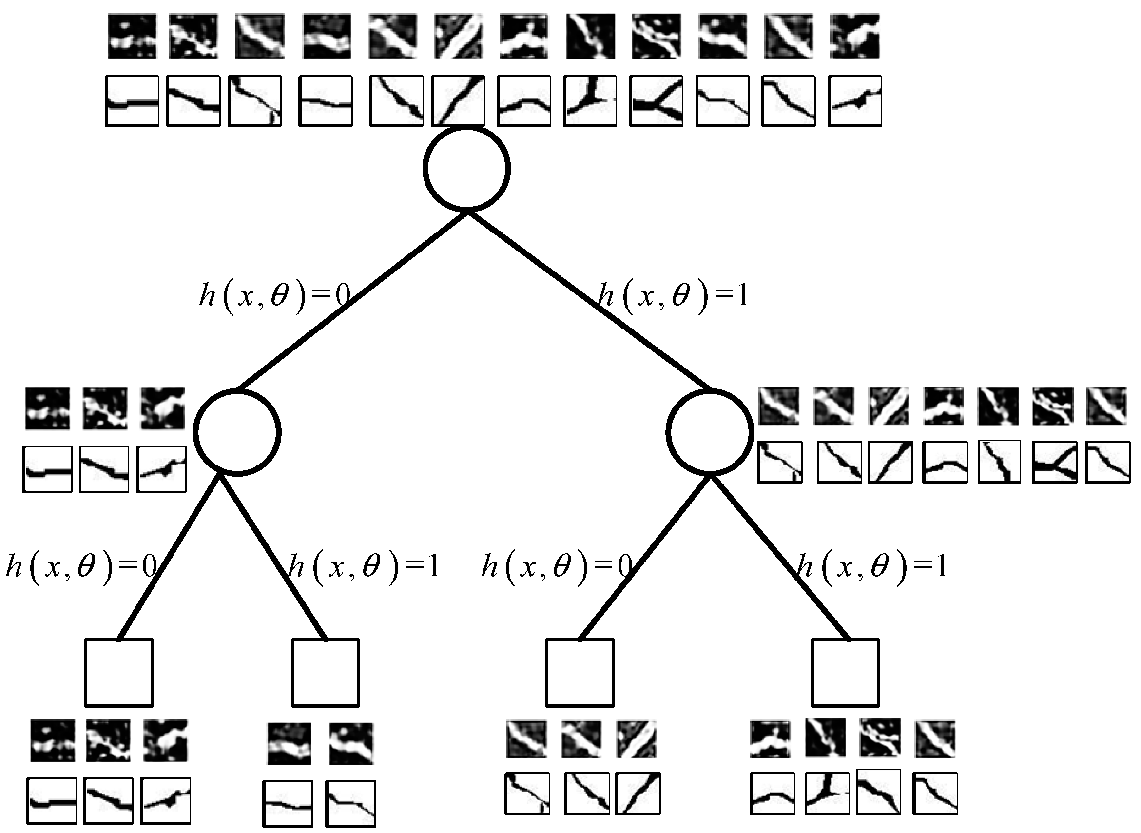
Construct a random structured forest using the channel features and structured labels of image blocks. The training of decision trees involves constructing prediction results for decision tree nodes (represented by circles in Figure 10) and leaf nodes (represented by rectangles in Figure 10). Constructing a decision tree starts from the root node and initializes the root node first. Node splitting is the core step in constructing a decision tree, and it is through node splitting that a complete decision tree can be generated. Each node $N(h,f_t^L,f_t^R)$ corresponds to a binary splitting function $h\left(x,\theta \right)\in \left\{0,1\right\}$. If sample $h\left(x,\theta \right)=0$, x reaches the left subtree of that node, and vice-versa, if it reaches the right subtree $f_t^R$ of that node, the splitting of the decision tree node occurs, as shown in Figure 10. When splitting nodes, the decision tree’s nodes are determined based on the maximum depth of the tree, the minimum number of samples, and the information gain of the samples. If the node no longer splits, it will serve as a leaf node, where the most representative structured label on the node will be used as the predicted result for the leaf node. If the node continues to split, all partitions of each attribute in the random feature subset are sorted according to the information gain, and then the attribute with the highest information gain is selected as the splitting attribute. The samples on the node are divided into samples from the left subtree and samples from the right subtree, and the branching growth of the decision tree is achieved based on their division until the node no longer satisfies the node splitting rule. The last node of each branch is considered a leaf node. For each leaf node, a structured label with the smallest distance from other structured labels as the decision result for that leaf node is selected. The process of constructing a random structure forest is shown in Figure 11.

After training the random structured forest, all representative structures are gathered on the leaf nodes of the decision trees. In the testing phase, a sliding window with a size of 16 × 16 is employed to extract image blocks corresponding to each pixel in the test image. The input image blocks start from the root node of the decision tree, and based on the splitting function of each node, they are routed from top to bottom until they finally point to a leaf node. Then, the most representative structured label on the leaf node is adopted as the prediction result of the decision tree for that image block, as illustrated in Figure 12. The circles in the figure represent decision tree nodes, rectangles represent leaf nodes, red branches represent selected paths, and the black marker at the end represents the decision result of the leaf node. Due to the prevalence of a large number of duplicate pixel points in the image blocks of adjacent pixels and their corresponding structured labels, the probability of each pixel being a cracked pixel is computed by taking the average of the repeated prediction results for each pixel point. Consequently, the output of the crack detector based on the random structured forest corresponds to a crack probability map, where the numerical value of each pixel signifies the probability that the corresponding pixel in the original road crack image represents a crack. Preliminary crack detection results can be obtained by applying threshold segmentation to the crack probability map.

2.4. Road Crack Recognition Method Based on Density Clustering

The basic idea of the pavement crack recognition method based on density clustering is to cluster crack candidate points into clusters of any topological structure and then select cracks based on their geometric characteristics. Road surface cracks have complex topological structures and poor continuity and are susceptible to noise interference in detection results. To tackle these challenges, this section introduces a crack identification approach incorporating density clustering.

DBSCAN (density-based spatial clustering of applications with noise) is a density-based clustering algorithm that can discover clusters of any shape in a noisy data space. The main idea of the DBSCAN algorithm is to classify data points into three categories based on the density distribution in the data space: core points, boundary points, and noise points. If a point has at least MinPts (the minimum number of neighboring points) within the Eps distance, it is considered a core point. Eps is the search radius, and MinPts is the minimum number of neighbors that the core point must have. If a point has fewer neighbors within the Eps distance than MinPts, but it is located within the Eps distance of a core point; then, the point is considered a boundary point. If a point does not belong to either the core point or the boundary point, it is considered a noise point. After repeated search processes, all points reachable through the core point are classified into clusters or marked as noise. Compared to other clustering methods such as k-means, spectral clustering, and rank order, this method can detect clusters of any shape without specifying the center point in advance or setting the initial number of clusters. It is robust to outliers and is an efficient, effective, and high-performance clustering algorithm [38]. In the process of crack detection, the adaptability of density clustering to irregular clusters is utilized to cluster the preliminary detection results obtained by the CrackForest model. The geometric characteristics of the clusters are then utilized to filter out the noise present in the preliminary detection results, thereby identifying the genuine pavement cracks. The crack extraction method based on density clustering mainly includes the following four steps:

(1)

Perform binarization on the crack probability map to obtain crack candidate points through threshold segmentation.

(2)

Perform density clustering on crack candidate points. Take all crack candidate points as a dataset and use the DBSCAN algorithm to cluster the crack candidate points. Firstly, examine a core point in the set of crack candidate points and generate a new object cluster centered on this core point. All data points in the Eps neighborhood of the core point are added to this object cluster, and these data points will serve as the objects to be examined next (referred to as seed points). Continuously explore the Eps neighborhood of seed points, expanding clusters until all density-connected points in the candidate set are identified. Generate other clusters using this method. Crack candidate points that have not been assigned to any cluster are considered noise points. Usually, the density of noise points is smaller than that of crack points; so, the DBSCAN algorithm can automatically filter out noise points and retain crack points by utilizing the density difference of crack points.

(3)

Extract the geometric features of each object cluster. The geometric features that need to be extracted mainly include the total number of pixels in the object cluster, the coordinates of extreme points in eight directions, and the pixel ratio between the object cluster and its smallest convex polygon. The total number of pixels in the object cluster reflects the size of the cluster area. By using the coordinates of the extreme points of the object cluster in eight directions, the longest distance of the object cluster in the four directions can be calculated. The pixel ratio between the object cluster and its smallest convex polygon reflects the reliability of the object cluster.

(4)

Using geometric features to classify various object clusters and accurately extract surface cracks. Although the DBSCAN algorithm can automatically filter out more scattered crack candidate points, some more concentrated and block-shaped crack candidate points may still be incorrectly clustered into crack clusters. Firstly, the coordinates of the extreme points in 8 directions of each crack cluster are queried so as to calculate the ratio of the shortest distance to the longest distance of each cluster. Taking advantage of the linear characteristics of road cracks, clusters with a ratio of the shortest distance to the longest distance greater than a specified threshold are identified as noise, thereby filtering out the true cracks and improving recognition accuracy.

3. Test Results

Experiments were conducted on two publicly available road crack datasets (CFD dataset and Cracktree200 dataset), manually labeling crack pixels in images as real reference values, extracting crack segmentation masks from the real reference values, and training crack detection models based on the crack segmentation masks. During the testing phase, the detection performance of the crack detection model was evaluated based on the real reference values. In order to quantitatively analyze and evaluate the effectiveness of crack extraction, this article used precision, recall, and F-1 values as evaluation indicators for experimental results. Their definitions can be found in Formulas (2)–(4), respectively.

$$Precision={\displaystyle \frac{TP}{TP+FP}}$$

(2)

$$\mathrm{Re}call={\displaystyle \frac{TP}{TP+FN}}$$

(3)

$$F1={\displaystyle \frac{2\times \mathrm{Pr}ecision\times \mathrm{Re}call}{\mathrm{Pr}ecision+\mathrm{Re}call}}$$

(4)

TP is the number of pixels correctly predicted as cracks by the model, FP is the number of pixels incorrectly predicted as cracks by the model, and FN is the number of pixels incorrectly predicted as non-crack by the model. Sometimes, there is a contradiction between precision and recall, and the F-1 value is the harmonic mean of precision and recall. In order to balance precision and recall, the F-1 value is used to comprehensively evaluate the overall performance of the model.

3.1. Impact of Key Parameters

When eliminating shadows, the purpose of performing morphological closure operations is to avoid mistakenly dividing road cracks into shadow areas. It is necessary to select structural elements of appropriate radius based on the width of the cracks. After multiple experiments, the radius of the structural elements was set to 27 pixels. This way, after performing closure operations, all cracks in the image can be removed. When dividing the brightness levels of shadow areas, the area of each brightness level area is too large, which can cause the image after brightness compensation to be overly unnatural. If it is too small, it may cause an inaccurate calculation of texture variance within a single brightness level area. In the experiment, it is required that the area of each shadow area is not less than 2% of the original image area. During the training of the random structure forest model, three main parameters were adjusted: the maximum depth of the decision tree MaxDepth, the minimum number of leaf nodes MinChild, and the threshold of the binary crack probability map threshold. Due to the lack of an optimal parameter generated based on optimization theory in the random structure forest algorithm, a series of experiments are needed to analyze the impact of these parameters on the overall performance of the crack detection model. This article used the F-1 value as a comprehensive indicator to evaluate the overall performance of the model; therefore, the F-1 value is the main indicator for selecting the optimal parameters.

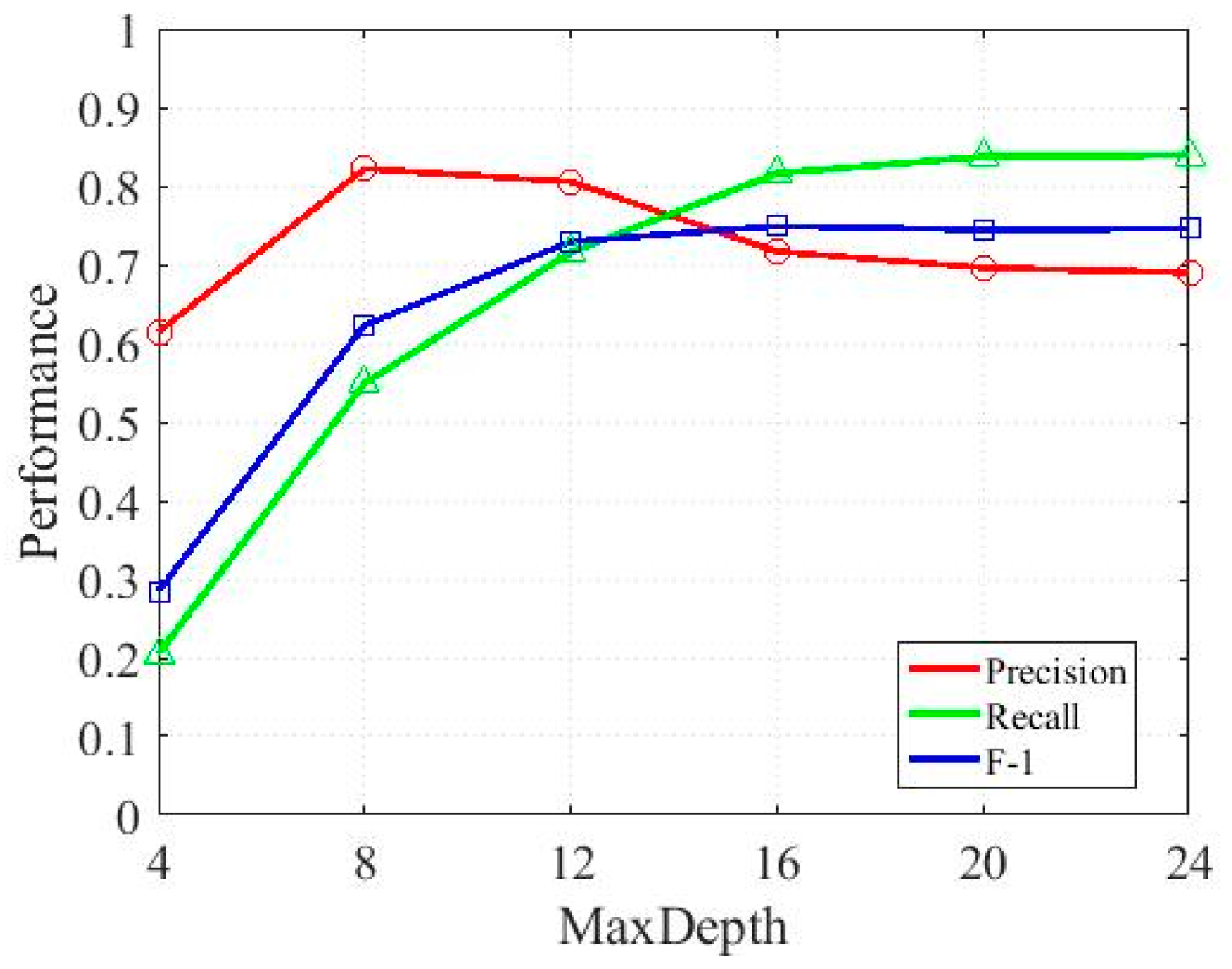
Firstly, we analyzed the impact of the maximum depth MaxDepth of the decision tree on the performance of the crack detection model. Due to the lack of pruning process in the random structure forest algorithm for generating decision trees, the size of the decision tree is mainly determined by its maximum depth. Setting the MaxDepth parameter too small can lead to the generated decision tree being too simple, insufficient model learning, and reduced accuracy in crack detection. Setting the MaxDepth parameter too large may lead to overfitting and reduce the model’s generalization ability. The authors will increase the parameter MaxDepth from 4 to 24, with a step size of 4. The curves of precision, recall, and F-1 values corresponding to different MaxDepths are shown in Figure 13. When MaxDepth increases from 4 to 16, both Recall and F-1 values rapidly increase, while precision begins to increase and slightly decreases from 12. When MaxDepth > 16, the precision value slightly decreases but does not change much, the recall value slightly increases and does not change much, while the F-1 value remains basically unchanged at around 0.74. Therefore, setting MaxDepth to 16, at which point the F-1 value is maximized, while the model can maintain a low error rate and avoid overfitting.

Due to the lack of pruning process, the minimum number of leaf nodes and the maximum depth of the decision tree jointly determine the splitting process of nodes in the decision tree. The minimum sample size of leaf nodes is too small, which may lead to overfitting in shallower nodes and insufficient splitting in deeper nodes, reducing the accuracy of the detection results. The minimum sample size of leaf nodes is too large, which will result in the generated decision tree being too simple and the samples on leaf nodes lacking representativeness. Firstly, we set the parameter MaxDepth = 16 and set the range of variation for the parameter MinChild to [2,20]. The impact of the MinChild parameter on the performance of the crack monitoring model is shown in Figure 14. When MinChild increases from 2 to 8, both precision and F-1 values rapidly increase, and when MinChild = 8, the maximum F-1 value is 0.74. At the same time, it can also be seen that, at that time, the F-1 values remained above 0.72, indicating that, when the parameter MinChild > 8, the node splitting in the decision tree was more sufficient, and the model was well trained. Overall, the crack detection model achieved the best crack detection results when MinChild = 8, with MinChild = 8.

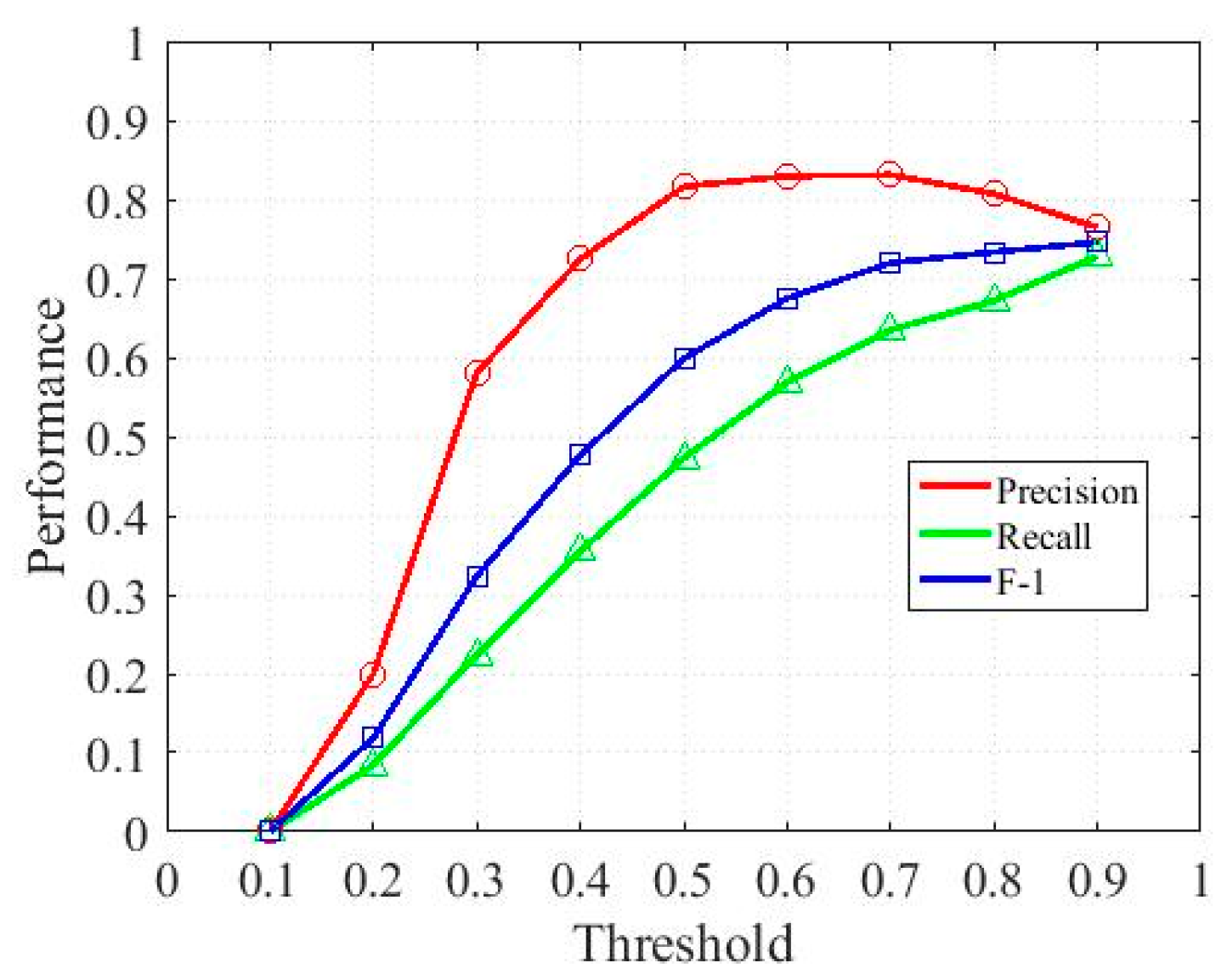
Finally, setting MaxDepth = 16 and MinChild = 8, the authors analyzed the impact of the parameter threshold on the model performance. Figure 15 shows the performance changes in the crack detection model when only the threshold value is changed. It can be seen that the F-1 value and recall generally increase with the increase in the parameter threshold, but precision decreases with the increase in threshold when the threshold is greater than 0.7. This is because the larger the threshold for the binarization of the crack probability map, the more likely the candidate crack points selected based on the crack probability map are to be true crack points, reducing the number of false counterexamples and obtaining a higher recall. From Figure 15, it can be seen that, when the parameter threshold = 0.9, the F-1 value and recall of the model reach their maximum values. Therefore, this article sets the threshold of the model parameters to 0.9.

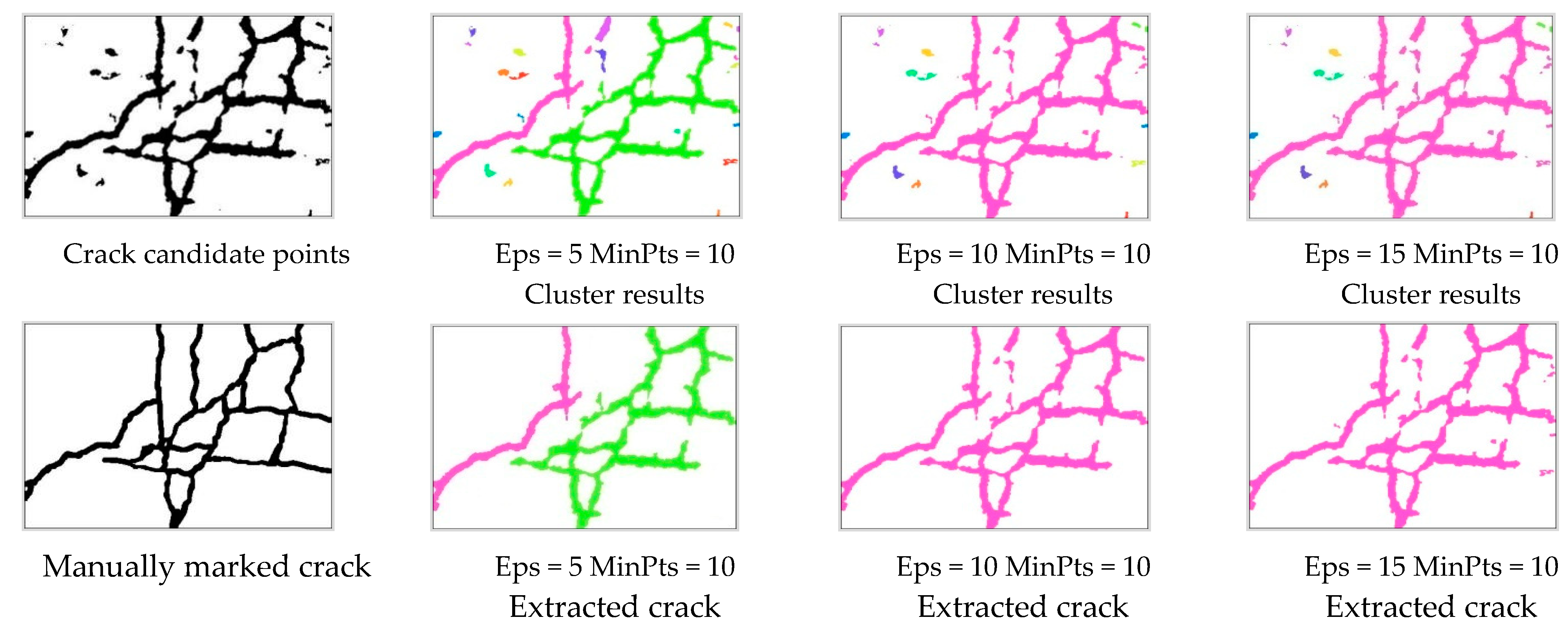
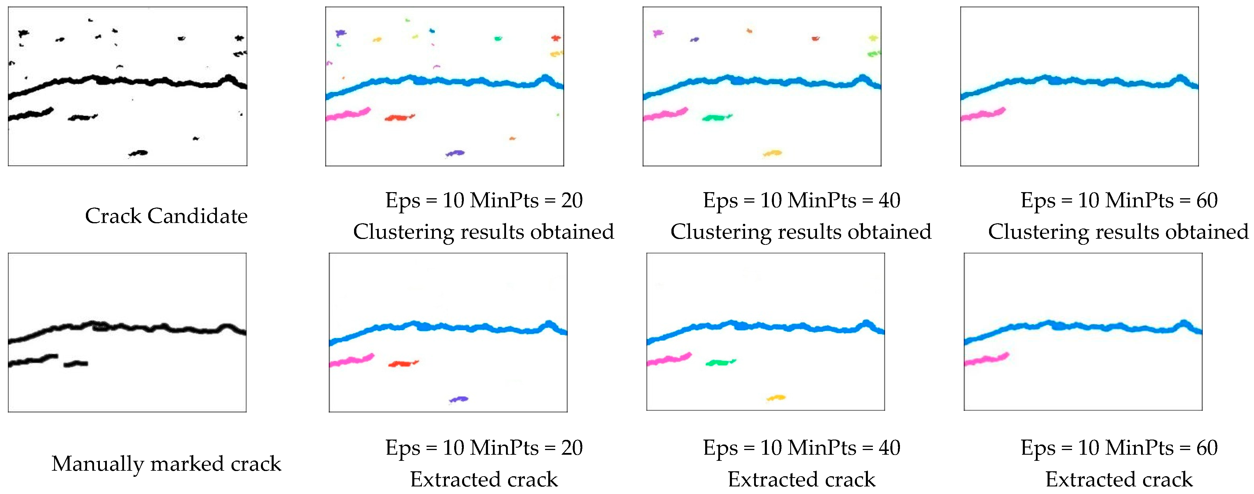
The key parameters that need to be adjusted when clustering crack candidate points using algorithms include neighborhood radius (Eps) and the minimum number of samples for clustering (MinPts). The algorithm requires users to manually set these two parameters, which directly affect the results of density clustering. To obtain good clustering results, it is necessary to choose appropriate parameters, which requires multiple experiments to obtain. By conducting experiments on the probability map of cracks in a typical road surface image, the parameters and their impact on the clustering results of crack candidate points can be visually displayed, as shown in Figure 16 and Figure 17. Different colors in the figure represent different clusters, while the same color represents that the crack candidate point is in the same cluster.

The first row of Figure 16 and Figure 17 shows the extracted crack candidate points from the crack probability map, as well as the density clustering results obtained with different parameters. In the figure, different object clusters are marked with different colors. The second rows of Figure 16 and Figure 17 show manually annotated road cracks and extracted road cracks based on different clustering results, respectively. From the graph, it can be seen that density clustering not only filters out scattered noise data, but also identifies various crack fragments belonging to the same crack as the same crack, thereby improving the continuity of crack detection results. Although the density aggregation of crack candidate points cannot filter out large areas of noise, utilizing the geometric features of object clusters can accurately identify cracks and noise, thereby accurately extracting surface cracks. From Figure 16 and Figure 17, it can be seen that the best crack detection results are achieved when the parameter is set to 10 pixels and 40, detecting all road cracks while minimizing the interference of noise on the crack detection results.

3.2. Test Results of Test Set

To verify the performance of the crack detection method proposed in this article, experiments were conducted on publicly available CFD pavement crack datasets and the Cracktree200 crack dataset. In the experiment, the code was written in Matlab(R2019b) and tested on the Windows 7 operating system with a CPU of 2.5 GHz. The CFD dataset contains 155 images of size, and all road crack images do not contain shadows. The authors used 110 of them as the training set and 45 as the test set. The Cracktree200 dataset contains 206 crack images of size, of which 36 road crack images contain shadows. The authors used 146 of them as the training set and the remaining 60 as the test set, keeping the training set and test set roughly balanced with the crack images containing shadows. Because cracks have a certain width, a tolerance width value of 2 pixels was set when determining whether they are crack pixels. When the Euclidean distance between the detection result and the manually labeled crack is 2 pixels, the authors considered it as a crack pixel.

Table 1. Precision, recall, and F-1 values of the comparative methods on the CFD datasets.

Method	Precision	Recall	F-1
CrackForest	0.558	0.76	0.643
UNet++	0.796	0.754	0.774
Deeplabv3+	0.823	0.792	0.807
Proposed method	0.874	0.839	0.856

lists the results obtained from comparative experiments on the CFD dataset. The proposed method in this paper achieved a precision of 0.874, recall of 0.839, and F-1 value of 0.856 for crack detection on the CFD dataset. Compared to the CrackForest model, the method proposed in this paper improved the precision by 56.6%, recall by 10.4%, and F-1 value by 33.1%. Compared to the latest and most widely used UNet++ and Deeplabv3+ algorithms in road crack detection, the precision of our method increased by 9.8% and 6.2%, the recall increased by 11.3% and 5.9%, and the F-1 value increased by 10.6% and 6.1%, respectively.

Table 2. Precision, recall, and F-1 values of the comparative methods on the Cracktree200 dataset.

Method	Precision	Recall	F-1
CrackForest	0.635	0.717	0.674
UNet++	0.789	0.766	0.777
Deeplabv3+	0.821	0.786	0.803
Proposed method	0.846	0.826	0.836

presents the results of comparative experiments conducted on the Cracktree200 dataset using the method proposed in this paper. The precision of crack detection using the algorithm proposed in this paper is 0.846, the recall is 0.826, and the F-1 value is 0.836. Compared to the CrackForest model, the method proposed in this paper improved the precision by 33.2%, recall by 15.2%, and the F-1 value by 24%. When compared to the UNet++ and Deeplabv3+ algorithms, the precision of our method increased by 7.2% and 3.0%, respectively; the recall increased by 7.8% and 4.8%, respectively; and the F-1 value increased by 7.6% and 4.1%, respectively.

Figure 18, Figure 19, Figure 20, Figure 21, Figure 22 and Figure 23 show the processing results of six representative road crack images from two road crack datasets. Figure 18 is the original image, Figure 19 is the detection result obtained by the CrackForest model, Figure 20 is the detection result of the UNet++ algorithm, Figure 21 is the detection result of Deeplabv3+, Figure 22 is the detection result obtained by the crack detection method proposed in this paper, and Figure 23 is the manually annotated crack. It can be seen that the cracks in the images of Figure 18a,b are relatively clear. Except for a small number of noise points detected by the CrackForest algorithm, the detection results of UNet++, Deeplabv3+ and our algorithm are close to the real results. Figure 18c,d There are oil stains and shadow interference in the Figure 18c,d, and the CrackForest algorithm incorrectly identifies the oil stains and shadows as cracks. UNet++ and Deeplabv3+ are also subject to certain interference, resulting in false positives and false negatives. However, the algorithm proposed in this paper overcomes the interference of oil stains and shadows through preprocessing, and the detection results are more accurate. Figure 18e,f Due to the influence of road surface materials, Figure 18e,f not only have shadows and oil pollution interference but also easily mistake noise for cracks. The CrackForest model detects a large number of false positive errors, and UNet++ and Deeplabv3++ detection results also have false positives and missed detections. In comparison, the algorithm proposed in this paper achieves better detection results. In summary, the results obtained by the method proposed in this article have good consistency with real cracks, and the detection results are not easily affected by interference factors such as road shadows and oil stains. The model has a good anti-interference ability, and the crack detection effect is not only better than the CrackForest model but also has higher precision, recall, and F-1 than most advanced road crack detection methods currently available.

4. Conclusions

This paper proposes a pavement crack detection method using CrackForest-based density clustering, which can detect complete cracks from pavement images with noises such as shadows and oil stains. Aiming at the problems of the difficult boundary definition of shadow areas and low contrast of cracks in shadow areas, this paper proposes a shadow removal method based on brightness division. Then, the CrackForest algorithm is used to construct a crack detector. The crack detector predicts and generates a crack probability map by structuring the road crack image after shadow removal. Finally, a density clustering-based crack extraction method is used to extract complete road cracks from the crack probability map. This crack detection method not only overcomes the influence of road surface shadows on crack detection results, but also effectively identifies noise and cracks in the road surface images, improving the accuracy and robustness of detection results. The method proposed in this article was tested on the CFD and Cracktree200 datasets, with precision reaching 87.4% and 84.6%, recall reaching 83.9% and 82.6%, and F-1 values reaching 85.6% and 83.6%, respectively. Through comparative experiments, it was found that the proposed road crack detection method not only significantly improved the precision, recall, and F-1 value compared to the CrackForest method, but also surpassed most other advanced road crack detection methods currently available.

The algorithm presented in this article has to some extent overcome noise interference and achieved the goal of detecting road cracks, providing technical support for the automated detection of road cracks and providing a new approach for research into shadow removal, feature enhancement, and feature extraction. This method has certain limitations in weak texture areas with discontinuous cracks and unclear textures. The authors also plan to further explore the applicability of the algorithm used in this article in identifying road surface distresses in different scenarios and improve the accuracy of detection.

References

1. Munawar, H.S.; Hammad, A.W.; Haddad, A.; Soares, C.A.P.; Waller, S.T. Image-based crack detection methods: A review. Infrastructures 2021, 6, 115. [Google Scholar] [CrossRef]
2. Amhaz, R.; Chambon, S.; Idier, J.; Baltazart, V. Automatic crack detection on two-dimensional pavement images: An algorithm based on minimal path selection. IEEE Trans. Intell. Transp. Syst. 2016, 17, 2718–2729. [Google Scholar] [CrossRef]
3. Walubita, L.F.; Faruk, A.N.; Zhang, J.; Hu, X. Characterizing the cracking and fracture properties of geosynthetic interlayer reinforced HMA samples using the Overlay Tester (OT). Constr. Build. Mater. 2015, 93, 695–702. [Google Scholar] [CrossRef]
4. Oliveira, H.; Correia, P.L. Automatic road crack detection and characterization. IEEE Trans. Intell. Transp. Syst. 2012, 14, 155–168. [Google Scholar] [CrossRef]
5. Walubita, L.F.; Mahmoud, E.; Lee, S.I.; Carrasco, G.; Komba, J.J.; Fuentes, L.; Nyamuhokya, T.P. Use of grid reinforcement in HMA overlays–A Texas field case study of highway US 59 in Atlanta District. Constr. Build. Mater. 2019, 213, 325–336. [Google Scholar] [CrossRef]
6. Han, C.; Ma, T.; Ju, H.; Huang, X.; Zhang, Y. CrackW-Net: A novel pavement crack image segmentation convolutional neural network. IEEE Trans. Intell. Transp. Syst. 2021, 23, 22135–22144. [Google Scholar] [CrossRef]
7. Chen, F.C.; Jahanshahi, M.R. NB-CNN: Deep Learning-based Crack Detection Using Convolutional Neural Network and Naïve Bayes Data Fusion. IEEE Trans. Ind. Electron. 2018, 65, 4392–4400. [Google Scholar] [CrossRef]
8. Liao, Y.P.; Wang, W.X. Improved Graph MST-Based Image Segmentation with Non-Subsampled Contourlet Transform. Huanan Ligong Daxue Xuebao/J. South China Univ. Technol. Nat. Sci. 2017, 45, 143–152. [Google Scholar]
9. Kahmann, S.L.; Rausch, V.; Plümer, J.; Müller, L.P.; Pieper, M.; Wegmann, K. The automized fracture edge detection and generation of three-dimensional fracture probability heat maps. Med. Eng. Phys. 2022, 110, 103913. [Google Scholar] [CrossRef]
10. Xu, D.; Zhao, Y.; Jiang, Y.; Zhang, C.; Sun, B.; He, X. Using Improved Edge Detection Method to Detect Mining-Induced Ground Fissures Identified by Unmanned Aerial Vehicle Remote Sensing. Remote Sens. 2021, 13, 3652. [Google Scholar] [CrossRef]
11. Xu, D.; Zhao, Y.; Jiang, Y.; Zhang, C.; Sun, B.; He, X. An image enhancement algorithm to improve road tunnel crack transfer detection. Constr. Build. Mater. 2022, 348, 128583. [Google Scholar]
12. Liu, X.; Ai, Y.; Scherer, S. Robust image-based crack detection in concrete structure using multi-scale enhancement and visual features. In Proceedings of the 2017 IEEE International Conference on Image Processing (ICIP), Beijing, China, 17–20 September 2017; pp. 2304–2308. [Google Scholar]
13. Peng, C.; Yang, M.; Zheng, Q.; Zhang, J.; Wang, D.; Yan, R.; Wang, J.; Li, B. A triple-thresholds pavement crack detection method leveraging random structured forest. Constr. Build. Mater. 2020, 263, 120080. [Google Scholar] [CrossRef]
14. Shen, L.; Wee Chua, T.; Leman, K. Shadow optimization from structured deep edge detection. In Proceedings of the IEEE Conference on Computer Vision and Pattern Recognition (CVPR), Boston, MA, USA, 7–12 June 2015; pp. 2067–2074. [Google Scholar]
15. Landabaso, J.L.; Pardàs, M.; Xu, L.Q. Shadow removal with morphological reconstruction. In Proceedings of the Jornades de Recerca en Automàtica, Barcelona, Spain, 4–6 July 2020. [Google Scholar]
16. Gong, H.; Cosker, D. User-assisted image shadow removal. Image Vis. Comput. 2017, 62, 19–27. [Google Scholar] [CrossRef]
17. Khan, S.H.; Bennamoun, M.; Sohel, F.; Togneri, R. Automatic shadow detection and removal from a single image. IEEE Trans. Pattern Anal. Mach. Intell. 2016, 38, 431–446. [Google Scholar] [CrossRef]
18. Liu, S.; Chen, M.; Li, Z.; Liu, J.; He, M. A differential correction based shadow removal method for real-time monitoring. PLoS ONE 2023, 18, e0276284. [Google Scholar] [CrossRef]
19. Wang, H.; Zou, H.; Zhang, D. Attentive Generative Adversarial Network with Dual Encoder-Decoder for Shadow Removal. Information 2022, 13, 377. [Google Scholar] [CrossRef]
20. Jongwoo, H.; Dongsoo, K.; Minsoo, K. Assessing severity of road cracks using deep learning-based segmentation and Detection. J. Supercomput. 2022, 78, 17721–17735. [Google Scholar]
21. Zhao, G.; Wang, T.; Ye, J. Anisotropic clustering on surfaces for crack extraction. Mach. Vis. Appl. 2015, 26, 675–688. [Google Scholar] [CrossRef]
22. Zheng, Q.; Tian, X.; Yang, M.; Wu, Y.; Su, H. Pac-bayesian framework based droppath method for 2d discriminative convolutional network pruning. Multidimens. Syst. Signal Process. 2020, 31, 793–827. [Google Scholar] [CrossRef]
23. Li, R.; Yu, J.; Li, F.; Yang, R.; Wang, Y.; Peng, Z. Automatic bridge crack detection using Unmanned aerial vehicle and Faster R-CNN. Constr. Build. Mater. 2023, 362, 129659. [Google Scholar] [CrossRef]
24. Yan, B.F.; Xu, G.Y.; Luan, J.; Lin, D.; Deng, L. Pavement distress detection based on faster r-cnn and morphological operations. China J. Highw. Transp. 2021, 34, 181. [Google Scholar]
25. Tran, T.S.; Tran, V.P.; Lee, H.J.; Flores, J.M.; Le, V.P. A two-step sequential automated crack detection and severity classification process for asphalt pavements. Int. J. Pavement Eng. 2022, 23, 2019–2033. [Google Scholar] [CrossRef]
26. Liu, Z.; Yeoh, J.K.; Gu, X.; Dong, Q.; Chen, Y.; Wu, W.; Wang, L.; Wang, D. Automatic pixel-level detection of vertical cracks in asphalt pavement based on GPR investigation and improved mask R-CNN. Autom. Constr. 2023, 146, 104689. [Google Scholar] [CrossRef]
27. Nguyen, N.H.T.; Perry, S.; Bone, D.; Le, H.T.; Nguyen, T.T. Two-stage convolutional neural network for road crack detection and segmentation. Expert Syst. Appl. 2021, 186, 115718. [Google Scholar] [CrossRef]
28. Hou, Y.; Chen, Y.H.; Gu, X.Y.; Mao, Q.; Cao, D.D.; Wang, L.B.; Jing, P. Automatic Indentification of Pavament Objects and Cracks Using the Convolutional Auto-encoder. China J. HighW. Transp. 2020, 33, 288–303. [Google Scholar]
29. Liu, P.; Yuan, J.; Chen, S. A road damage segmentation method for complex environment based on improved UNet. In Proceedings of the International Conference on Image and Graphics, Beijing China, 19–21 January 2023; Springer Nature: Cham, Switzerland, 2023; pp. 332–343. [Google Scholar]
30. Sun, X.; Xie, Y.; Jiang, L.; Cao, Y.; Liu, B. DMA-Net: DeepLab with multi-scale attention for pavement crack segmentation. IEEE Trans. Intell. Transp. Syst. 2022, 23, 18392–18403. [Google Scholar] [CrossRef]
31. Shi, Y.; Cui, L.; Qi, Z.; Meng, F.; Chen, Z. Automatic Road Crack Detection Using Random Structured Forests. IEEE Trans. Intell. Transp. Syst. 2016, 17, 3434–3445. [Google Scholar] [CrossRef]
32. Nowozin, S.; Lampert, C.H. Structured Learning and Prediction in Computer Vision., Found. Trends® Comput. Graph 2010, 6, 185–365. [Google Scholar] [CrossRef]
33. Kontschieder, P.; Bulò, S.R.; Bischof, H.; Pelillo, M. Structured class-labels in random forests for semantic image labelling. IEEE Int. Conf. Comput. Vis. ICCV 2011, 11, 6–13. [Google Scholar]
34. Dollar, P.; Zitnick, C.L. Fast Edge Detection Using Structured Forests. IEEE Trans. Pattern Anal. Mach. Intell. 2015, 37, 1558–1570. [Google Scholar] [CrossRef]
35. Xu, Z.; Che, Y.; Min, H.; Wang, Z.; Zhao, X. Initial Classification Algorithm for Pavement Distress Images Using Features Fusion; Springer International Publishing AG: Cham, Switzerland, 2019; pp. 418–427. [Google Scholar]
36. Zhang, D. Crack detection for bituminous pavements based on cluster and minimum spanning tree. Zhongshan Daxue Xuebao/Acta Sci. Natralium Univ. Sunyatseni. 2017, 56, 68–74. [Google Scholar]
37. Dollár, P.; Zitnick, L.C. Structured Forests for Fast Edge Detection. In Proceedings of the 2013 IEEE International Conference on Computer Vision, Sydney, Australia, 1–8 December 2013; pp. 1841–1848. [Google Scholar]
38. Kremers, B.J.; Citrin, J.; Ho, A.; van de Plassche, K.L. Two-step clustering for data reduction combining DBSCAN and k-means clustering. Contrib. Plasma Phys. 2023, 63, e202200177. [Google Scholar] [CrossRef]
Figure 1. Research framework.
Automation 05 00027 g001
Figure 2. Images that require preprocessing.
Automation 05 00027 g002
Figure 3. Closing operation.
Automation 05 00027 g003
Figure 4. Gaussian filtering.
Automation 05 00027 g004
Figure 5. Brightness level division of the shadow area.
Automation 05 00027 g005
Figure 6. Image after brightness compensation.
Automation 05 00027 g006
Figure 7. Image after denoising and contrast enhancement.
Automation 05 00027 g007
Figure 8. Flowchart of the crack detection model.
Automation 05 00027 g008
Figure 9. Processed image effect (a) Image block. (b) Figure channel characteristics. (c) Split mask.
Automation 05 00027 g009
Figure 10. Decision tree node split.
Automation 05 00027 g010
Figure 11. The process of random structure forest.
Automation 05 00027 g011
Figure 12. Prediction of random structured forests.
Automation 05 00027 g012
Figure 13. Influence of the parameter MaxDepth on the performance of the crack detection model.
Automation 05 00027 g013
Figure 14. Influence of the parameter MinChild on the performance of the crack detection model.
Automation 05 00027 g014
Figure 15. Influence of the parameter threshold on the performance of the crack detection model.
Automation 05 00027 g015
Figure 16. Parameter influence on the crack extraction results.
Automation 05 00027 g016
Figure 17. The influence of the parameter MinPts on the crack extraction results.
Automation 05 00027 g017
Figure 18. Original image. (a) Example 1 of Ordinary Cracks (b) Example 2 of Ordinary Cracks (c) Image of cracks with oil stains (d) Image of cracks with shadows (e) Crack images with shadows and noise (f) Crack images with oil stains and noise.
Automation 05 00027 g018
Figure 19. CrackForest model detection results.
Automation 05 00027 g019
Figure 20. UNet++ detection results.
Automation 05 00027 g020
Figure 21. Deeplabv3+ detection results.
Automation 05 00027 g021
Figure 22. The test results of the method proposed in this paper.
Automation 05 00027 g022
Figure 23. Manual labeling results.
Automation 05 00027 g023