Digital Twin of a Flexible Manufacturing System for Solutions Preparation

Abstract

In the last few decades, there has been a growing necessity for systems that handle market changes and personalized customer needs with near mass production efficiency, defined as the new mass customization paradigm. The Industry 5.0 vision further enhances the human-centricity aspect, in the necessity for manufacturing systems to cooperate with workers, taking advantage of their problem-solving capabilities, creativity, and expertise of the manufacturing process. A solution is to develop a flexible manufacturing system capable of handling different customer requests and real-time decisions from operators. This paper tackles these aspects by proposing a digital twin of a robotic system for solution preparation capable of making real-time scheduling decisions and forecasts using a simulation model while allowing human interventions. A discrete event simulation model was used to forecast possible system improvements. The simulation handles real-time scheduling considering the possibility of adding identical parallel machines. Results show that processing multiple jobs simultaneously with more than one machine on critical processes, increasing the robot speed, and using heuristics that emphasize the shortest transportation time can reduce the overall completion time by 82%. The simulation model has an animated visualization window for a deeper understanding of the system.

1. Introduction

During the last few decades, remarkable scientific advancements in some digital technologies have led to new autonomous and self-regulated systems. These developments have increased the industry output capacity, but the growing variety and rising customer demand for individual or custom-made products at lower costs call for the design and operation of systems capable of handling this increasing variety of products [1]. This need to deliver products and services that best meet the individual customer’s needs with mass production efficiency is the mass customization trend [2]. A way to deal with this issue is to use flexible manufacturing systems (FMS), in which the system is built a priori to deal with changes in the market demands, able to yield a wide range of products from a single base unit [3,4].

The need to increase production flexibility, resilience, and sustainability of the industries is part of the ideals of Industry 5.0, as well as having closer cooperation between man and autonomous machines, taking advantage of the human problem-solving capabilities to increase the production flexibility, defined as human centricity [5,6].

This paper addresses the need for mass customization and flexible robust systems by developing a digital twin of a flexible manufacturing system for solution preparation capable of handling different requests and real-time changes from operators and clients using new technological trends.

The general idea of a digital twin refers to a comprehensive physical and functional description of a component, product, or system, corresponding to a digital replica, considered a twin, that allows the exchanging of information between the real system and its digital counterpart [7]. The digital twin coupled with data analytics allows for real-time monitoring, rapid analysis, and real-time decisions, allowing stakeholders to quickly detect problems in physical systems, increase the accuracy of their results, and more efficiently produce better products [8]. The concept was first introduced by Grieves [9] in 2002, and it was initially called “Conceptual Ideal for Product Lifecycle Management.” Although it did not have the current name, it shared the elements of a digital twin, including real space, virtual space, and links for data flow between both spaces. Summarily, these are the physical product, the digital replica, and their real-time connectivity. The term itself originated from the National Aeronautical Space Administration (NASA), which defined it as “A digital twin is an integrated multiphysics, multiscale, probabilistic simulation of an as-built vehicle or system that uses the best available physical models, sensor updates, fleet history, etc., to mirror the life of its corresponding flying twin” [10].

Among the challenges to deploying flexible manufacturing systems are the scheduling operations and the efficient use of the resources [11]. To make real-time scheduling decisions, the digital twin must be coupled with a decision support system that receives information from the real asset, using sensor technologies and business data to make scheduling decisions [12]. Scheduling in this context has the goal of assigning a set of jobs. Each job has a set of operations that need to be scheduled in machines to reduce the total time to process all the jobs (makespan) and increase machine utilization. As in the real world, machines can break down, orders can be late, operators might be unavailable, new urgent orders might arrive, and variations in processing time make the scheduling plan obsolete very quickly, especially in flexible systems [13]. The three most common scheduling approaches to deal with this issue are:

• Completely reactive scheduling: No firm schedule is made in advance, and all decisions are in real time. The decisions are made using a dispatching rule to select the next job with the highest priority from a set of available jobs waiting to be processed [14,15].
• Robust proactive scheduling: The concept in this approach revolves around creating predictive schedules by studying the main causes of disruptive events. The disruptions are measured based on actual versus planned completion. These disruptions are mitigated through a simple adjustment to the activities’ durations [16].
• Predictive–reactive scheduling: This is the most common of the three. The main idea is to build an initial baseline schedule to optimize the shop performance without considering disruptions. Afterward, this schedule is modified during execution, responding to real-time events [17].

To improve the resource utilization of the data-driven manufacturing system, a simulation model was created to test different resource configurations and scheduling scenarios. Coito et al. [18] first mentioned this manufacturing system for liquid solution preparation as part of a case study in a quality-control laboratory of the pharmaceutical industry. The authors proposed a platform that allows for the autonomous acquisition and management of personalized data in real time for mass customization manufacturing environments that supports the integration of dynamic decision support systems that can work together with the digital twin. 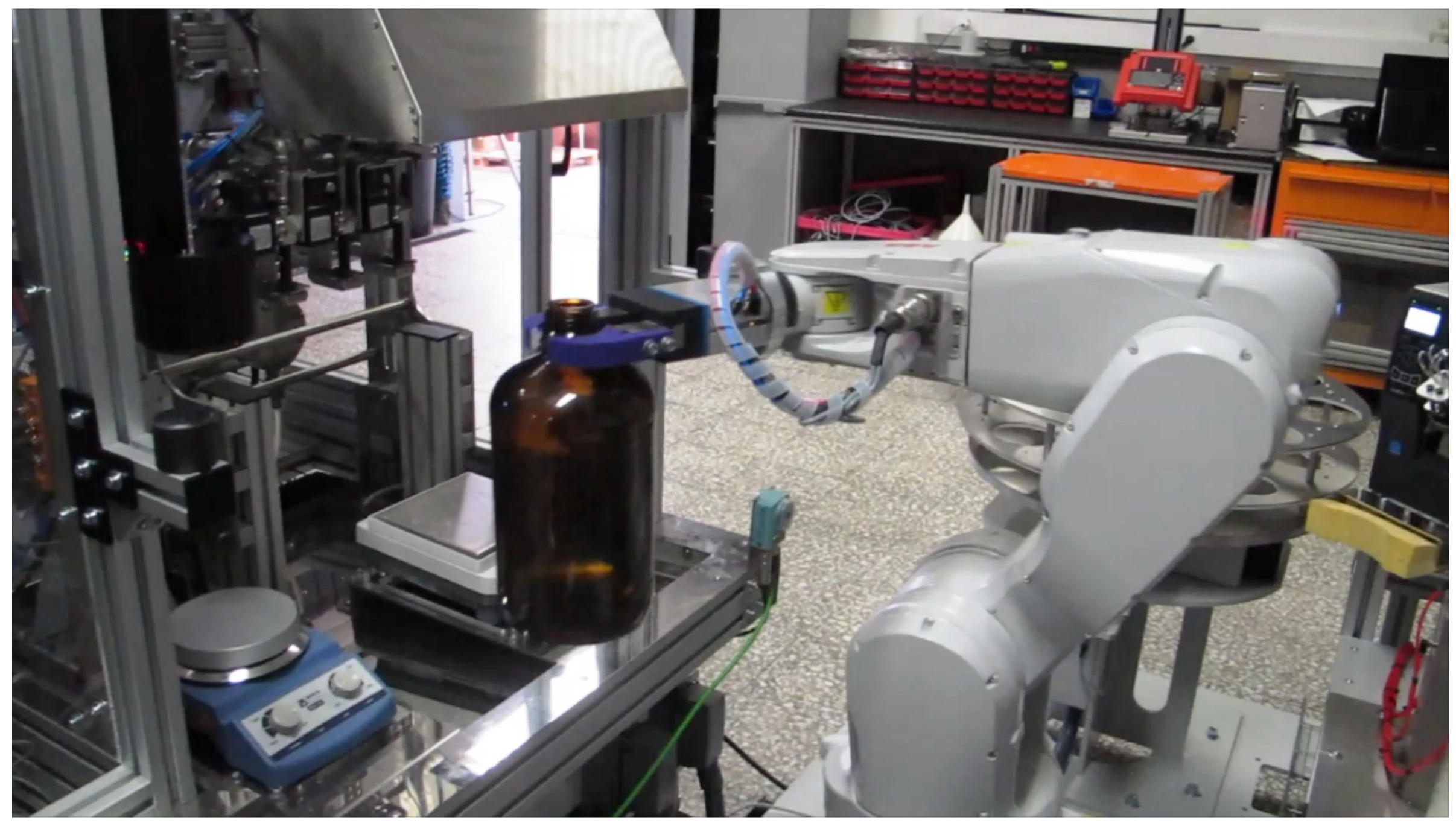Figure 1 represents the actual physical flexible manufacturing system used as the use case.

The robot system for solution preparation consists of an anthropomorphic robot with eight different workstations (Ws) with unique functions such as mixing, labeling, and stirring. These are within the robotic arm’s range, with the robot being the resource responsible for the movement of the bottles.

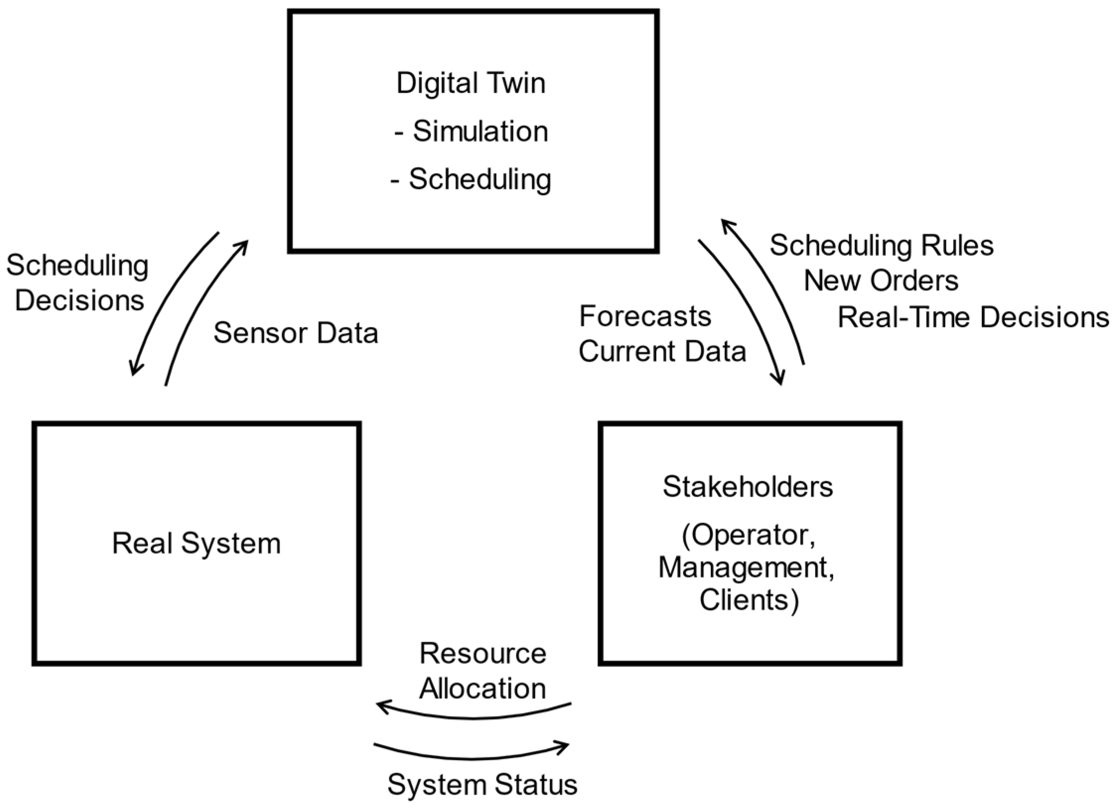
The system processes a single bottle or job at a time. The expectation is to reduce the makespan by having multiple jobs processed in parallel, adding extra machines in bottleneck tasks, changing robot parameters, and using the right scheduling algorithm. A system that handles multiple personalized jobs simultaneously and different customer requests while allowing stakeholders to manipulate processes, schedule parameters, and make real-time decisions creates the desired flexible environment. This paper focuses on simulating the environment comprised of the real system, stakeholders, and the DT (Figure 2).

Human centricity is achieved by having operators evaluate and monitor each production stage safely while providing expert knowledge in real time, such as changing the duration of tasks or the workflow.

Table 1. Data exchanged between the real system, stakeholders, and the digital twin.

Flow of Data	Data	Description
Real system → Digital twin	Sensor data	Events with the beginning and finishing timestamps of all tasks running in workstations and the robot.
Digital twin → Real system	Scheduling decisions	Orders the robot to complete movements and start tasks in workstations based on selected scheduling rules.
Real system → Stakeholders	System status	Visual execution of tasks and system diagnostics with stack lights.
Stakeholders → Real system	Resource allocation	Adding or removing resources. Inserting and removing bottles. Executing maintenance tasks.
Digital twin → Stakeholders	Forecasts Current data	Provides structured data of the real system, which allows models to be developed. Information on ongoing tasks and jobs. Provides KPIs such as the overall equipment effectiveness (OEE).
Stakeholders → Digital twin	Scheduling rules New orders Real-time decisions	Analysts can change the scheduling rules, control the list of jobs waiting to execute, and change the duration of tasks or the workflow in real-time.

summarizes the data exchanged between the real system, the digital twin, and the stakeholders. Details on the information exchanged between the real system and the digital twin are presented in Section 3.1.

The digital twin receives both historical and real-time data associated with the process flow of the manufacturing system, such as processing times, transportation times, and user actions. These data are used to make scheduling decisions based on a chosen algorithm. The digital twin can work as a tool to help stakeholders forecast asset improvements through simulation, such as to decide scheduling parameters, to determine where resources should be allocated, and to make real-time scheduling decisions with the constant flow of information from its real counterpart.

This paper provides a methodology to analyze the behavior of flexible cyber-physical production systems using a digital twin, considering mass customization and real-time changes from workers both involved in the topic of Industry 5.0. Contributions include:

• A digital twin focused on the simulation of a manufacturing system intended to make real-time scheduling decisions and forecast the system’s behavior for desired inputs and parameters such as client requests, heuristics, and resource configurations to better understand where the system can be improved.
• Proposes a human-centric approach to inspect personalized production and make decisions in real time.

This paper is structured as follows: In Section 2, the related work is presented on digital twins and discrete event systems used in the simulation. Section 3 details the system and the modeling architecture, followed by its implementation in a simulation model of the digital twin. Section 4 presents the data collection process and then the validation of the simulation model. Section 5 shows the results and analysis from the simulation study. In Section 6, the conclusions and future work are presented.

2. Related Work

2.1. Digital Twin

Digital twins can be applied to a broad range of areas, such as in health care, creating a virtual replica of a patient condition [19]; in smart cities, such as creating a 3D model of a city with the energy consumption and renewable energy production of everything [20]; in logistics, to determine the optimal flow between facilities to maximize productivity [7] or in port operations [21]; in manufacturing, such as allowing the visualization of how production lines are producing, allowing for real-time monitoring and manipulation of process parameters and optimization [22]; and sometimes merging areas such as manufacturing and logistics, using data from processes, personnel, and equipment, collected using Industrial IoT, and then using that information together with decision support systems to change routes [7,23].

Focusing on manufacturing implementations, Kunath et al. [24] developed a digital twin of a manufacturing system integrated with a decision support system to improve the management of the production orders. The decision support system automatically generated and built simulation models using information from the digital twin and all relevant business data for decision-making in real time. Using intelligent and self-learning search algorithms, the decision support system improved the overall performance of the company and the whole supply chain. Regarding flexible production, Havard et al. [25] combined the concepts of digital twin and virtual reality with the transportation assured by mobile robots. The digital twin combined with virtual reality allowed engineers and operators to test various configurations and give feedback with realistic behavior of the manufacturing system. To test the increase in productivity of a new automation solution, Karagiannis et al. [1] developed a discrete event system (DES) model. The simulation model offered the possibility of testing all the probable occurrences in the assembly line by manipulating the parameters in a risk-free virtual environment.

The most similar manufacturing system identified in the literature, compared to ours, was presented by Park et al. [26], who proposed a digital twin-based cyber-physical production system. Similarly, the system pivoted around a central robot with modular stations positioned in an octagon formation for personal production in a “micro-factory” setting. However, the authors developed an architectural framework of the system, focusing on preventing performance degradation.

Regarding improving the resource utilization and test difference scheduling policies, Lopes et al. [27] developed a digital twin of the quality-control laboratory to assist managers in the tasks of resource planning and scheduling. The authors implemented a discrete-event simulation model. The model was used as a testing platform to benchmark alternative governance models, scheduling heuristics, and resource allocation policies intended to be deployed. Coito et al. [28] also developed a digital twin of an improved version of the quality-control laboratories to assess the impact of automation in pharmaceutical quality control. The authors compared the current as-is and future to-be workflows, reworking the affected tasks using historical data to project increases in the availability of analysts and resources in different scenarios. Yu et al. [29] fused a digital twin with job shop scheduling of a flexible manufacturing system. The authors created a scheduling cloud platform that takes input from the sensors from the physical workshop, fuels data to its respective digital twin, and originates a fault prediction and diagnosis curve. The digital twin then gives simulation data and energy consumption diagrams to the scheduling platform to help plan the process steps. The authors found it advantageous to have access to a lot of data from the whole manufacturing process, helping to monitor the whole life cycle of the products, reduce energy consumption, and predict failures in the processes.

2.2. Discrete Event Systems

In the literature, digital twins often appear intertwined with simulation models. Computer simulation is a powerful tool used to analyze the performance of existing or newly designed systems by using mathematical or numerical techniques. Simulation works by creating a model of the conceptual framework of the system that can be used for a wide variety of experiments by analyzing simulation results. Conclusions can help stakeholders in the decision-making process [30]. One type of simulation already mentioned is discrete event modeling, where changes in the system occur at discrete times. These changes then affect the system depending on the chosen time advance mechanism (TAM). The two most common TAMs currently in use are the “next event” method, implemented in discrete event simulations (DES), and the “time step” or “fixed increment” method implemented in discrete time simulations (DTS) [30,31,32].

Real time is continuous, but a digital computer would take an infinite amount of time to represent it. In DTS, a “simulation clock” is introduced to sample time and make it finite. Time discretization works by incrementing constant time intervals (e.g., second, hour), effectively “skipping time” between increments. This way, continuous times are simulated on digital computers [31]. Contrary to DTS, in discrete event systems (DES), the state transitions are driven by the combination of asynchronous and concurrent events. This way, events are the cause of change in the system, so the concept of time is not the driving force of the simulation and is instead a variable dependent on the state transitions. So, the simulation effectively skips time between events [33].

There is a lack of research on using digital twins for real-time decision-making to reduce the makespan of a flexible manufacturing system by evaluating and improving the equipment utilization with a simulation model in a human-centric personalized production environment—more specifically, when the transportation element between workstations is a robotic arm. Additionally, the literature presents stochastic conditions, machine breakdowns, new orders, late arrivals, and workers unavailable as properties that make the system dynamic. However, it does not sufficiently consider the inclusion of a human counterpart capable of changing processing times and workflow and the flexibility introduced by a flexible manufacturing system for custom production [16,17,34].

Therefore, the research question is how to improve a flexible manufacturing system for custom production using a digital twin, particularly, a manufacturing system where the transportation element is a robot and human collaboration is allowed.

3. Digital Twin of a Robotic System for Solution Preparation

3.1. Methodology

To improve flexible manufacturing systems for custom production using a digital twin, the methodology was adopted to answer the research question in five steps:

• Modeling of the actual system;
• Creation of the digital twin;
• Creation of a discrete event simulation model;
• Testing different scenarios;
• Identifying improvement opportunities.

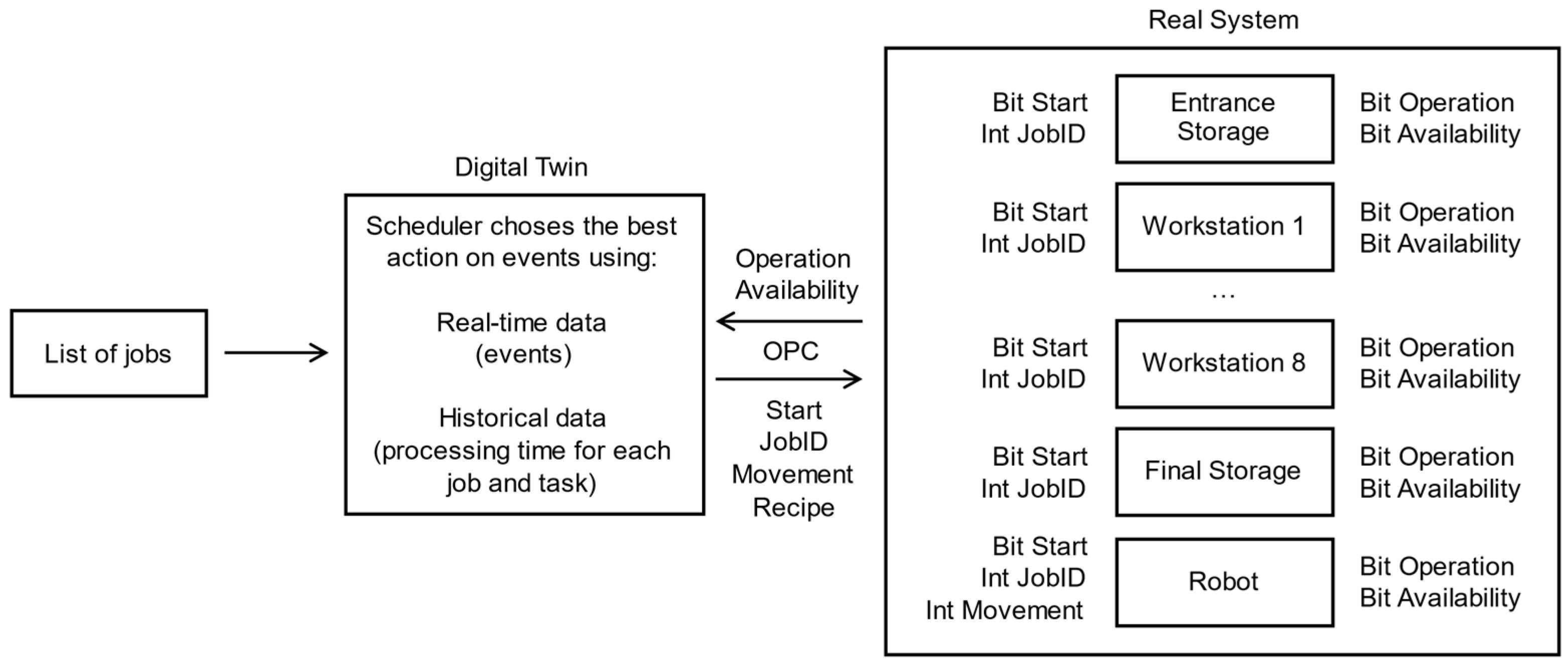
The proposed modeling approach uses the business process model and notation (BPMN). BPMN is a graphical framework to represent system workflows, narrowing the gap between actual systems and monitoring activities [35]. With BPMN, each job task is modeled as a process. In a digital twin, the beginning and end of each task in a workstation are tracked via OPC communication and exchanged with a decision support system in real time. The decision support system is event based, storing the information in a database, determining what to do next, and replying with an action via OPC. The bidirectional real–virtual data transmission is explained in Figure 3.

In Figure 3, each workstation and the robot have two bits associated:

• Operation status: 1 if a task is running in the workstation/robot, 0 if not.
• Availability status: 1 if the workstation/robot is occupied, 0 if not.

Although both appear to be similar, the operation may have finished (operation = 0) while the workstation is still occupied (availability = 1). Consider the situation in which the workstation has finished and waits for the bottle to be picked. The robot needs to know that that workstation is not free to do another job.

The digital twin combines real-time information from both bits with ongoing recipe data and past historical data from similar jobs to compute the expected processing time for all tasks and movements. Then, the selected scheduling rules decide the most efficient course of action.

There is also a Start bit to control the execution of tasks, along with a JobID taking an integer number. Additionally, the robot takes an integer number to tell which movement it should do. Recipe data are also sent to some workstations, such as quantities and working time.

Next, the strategy is to create a data-driven discrete event simulation model of the production workflow to test different scenarios. In the discrete event simulation approach, the model receives personalized jobs as input. These are taken randomly from an input list computed a priori from the digital twin data. With each job is associated a corresponding workflow, the duration of each process, and the human interventions. Each process has a processing time that follows a probabilistic distribution based on the digital twin data of the real case study. Processes require resources to run. Additionally, the decision support systems adopted in the digital twin are also modeled in the simulation model.

Finally, by testing different resource configurations, scheduling policies, human interventions, and decision support strategies, we can forecast possible improvements to the production for different demands, relying on the digital twin data.

The case study is a real manufacturing system for personalized production of solutions in the chemical and pharmaceutical industries that needs to be evaluated for possible improvements. The next section explains the model architecture of the digital twin and the discrete event simulation model, explaining the workflow and the decision algorithms, followed by the implementation.

3.2. Digital Twin Architecture

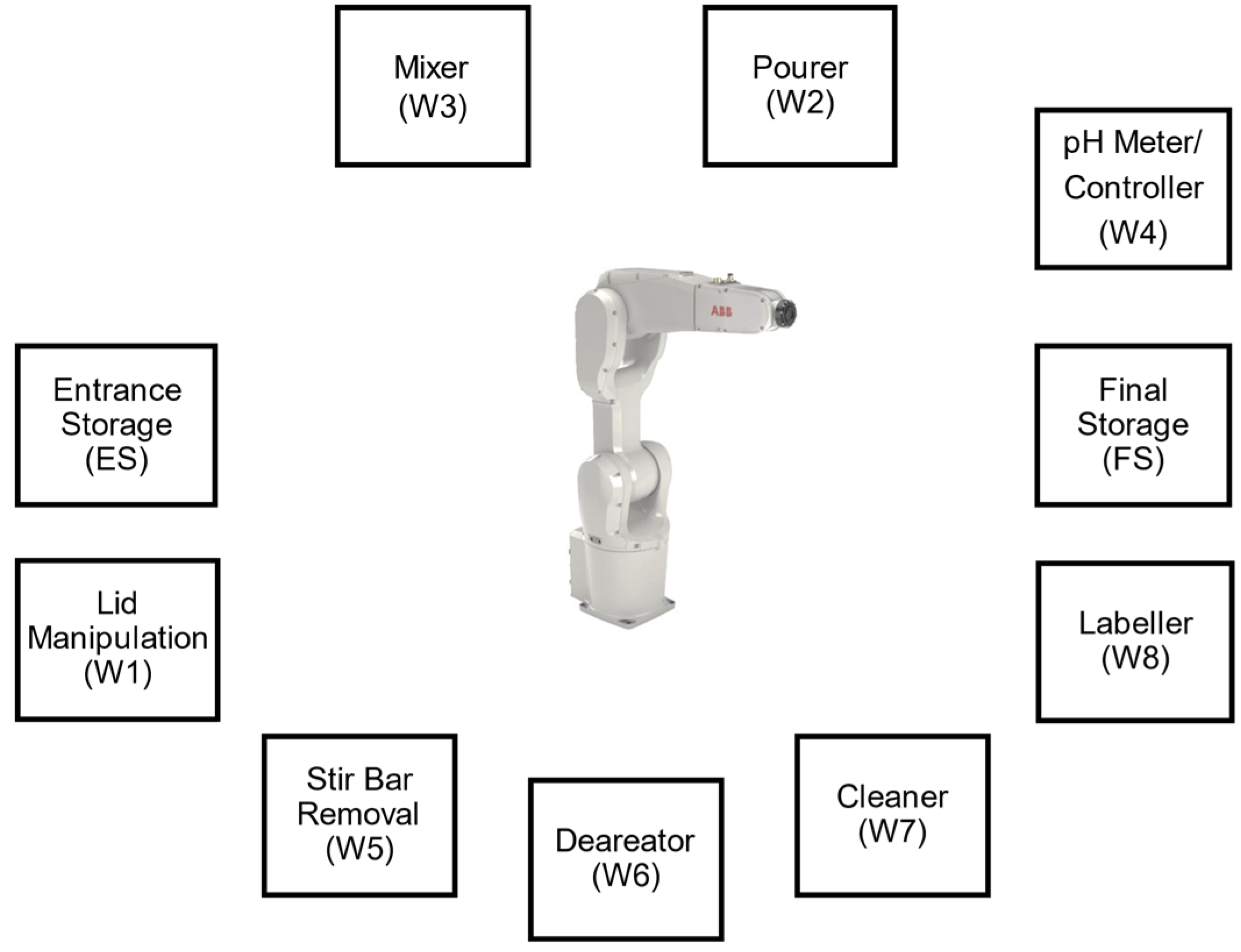
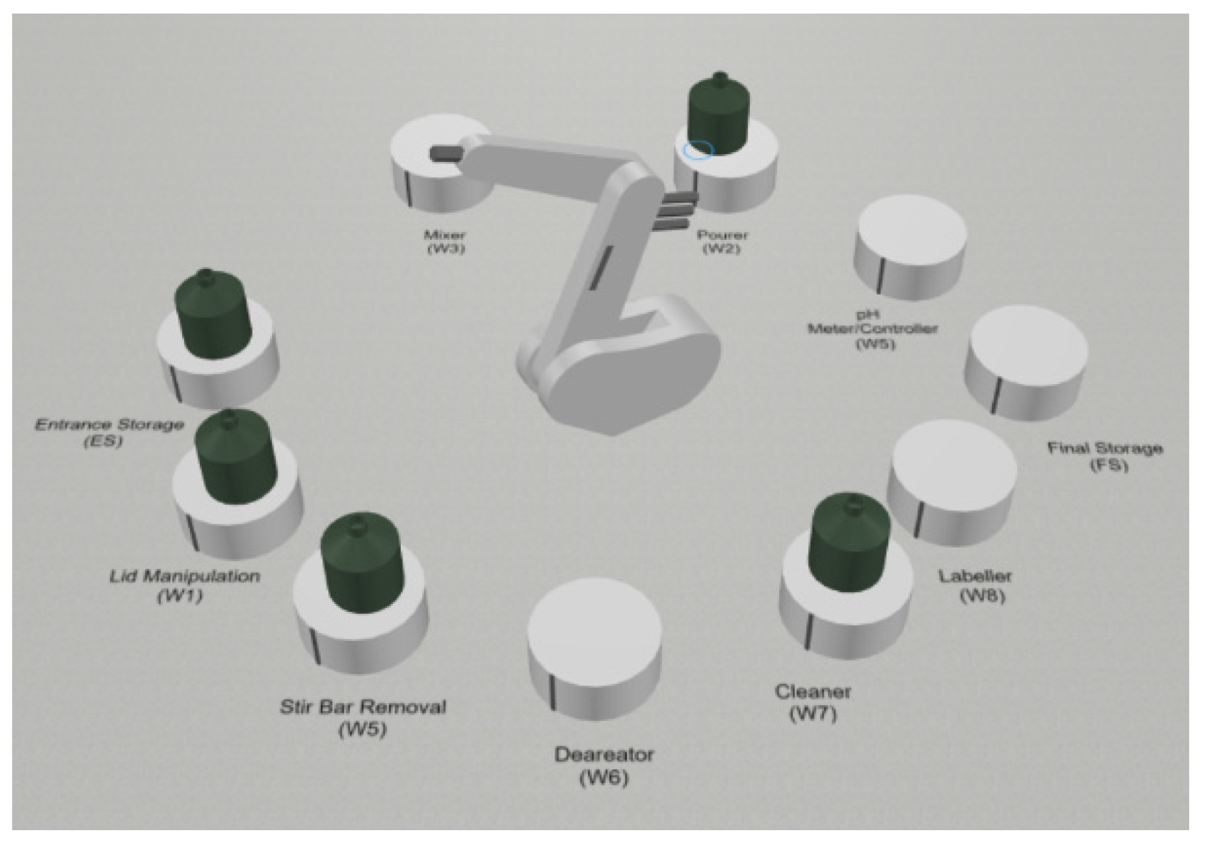
In the flexible manufacturing system for solution preparation, a bottle is considered an entity that goes through a sequence of workstations following a personalized request or job. Each workstation corresponds to a task and is modeled as a BPMN process with a processing time that follows a random probabilistic distribution. Generically, bottles are placed empty in the entrance storage (ES). Next, a robotic arm is responsible for moving each bottle through the workstations where the operations are executed until it ends up in the final storage (FS). The bottle finishes with the liquid solution inside. Both the ES and the FS use a rotating storing device. The workstations (Ws) and their positions relative to the robot are displayed in Figure 4.

Each movement of the robot is also considered a process $M_{ii,}$. The first one, $M_{01}$, describes the movement from the ES to workstation 1 (W1), $M_{12}$ from W1 to W2, and so on. Each recipe follows its own workflow, where the bottle can repeat or skip some of the tasks, depending on personalized requests and real-time decisions. In total there are 13 main movements with the bottle.

• Fetch an empty bottle from storage (ES) and place it in the cap manipulator (W1).
• Remove the cap (W1) and place it in the filling station (W2).
• After all the liquid is poured (W2), move the bottle to the mixing station (W3).
• Move the bottle from the mixing station (W3) to the pH controller (W4).
• After pH correction (W4), mix the solution again (W3).
• Move from the mixing station (W3) to the station where the stirrer is removed (W5).
• After the stirrer is removed (W5), go to the pre-tightening of the cap (W1).
• Move from pre-tightening the cap (W1) to the deaerator station (W6).
• After the deaerator (W6), move to the station to clean the outside of the bottle (W7).
• Move from the cleaning station (W7) to the final tightening of the cap (W1).
• After full tightening of the cap (W1), move to the printer and labeling station (W8).
• After labeling (W8), move the bottle to final storage (FS).
• When labeling is unnecessary, move from the cap station (W1) to final storage (FS).

The initial software developed for the solution preparation system only allowed for one job to be executed at a time. A new job could start only after the previous one was finished. To improve the workstations and robotic arm usage, the expectation is that the flexible manufacturing system must be able to run multiple jobs simultaneously. Bottles can move between workstations as long as it does not lead to blockage of the ongoing jobs. This flexibility means the robotic arm can do all possible combinations of movements between workstations when not carrying a bottle, moving between jobs. Additionally, it can go through the home position for calibration at any time.

Every time the robot finishes placing a bottle in a workstation, a dispatching rule determines the robot’s next movement. The robot can move without carrying a container when changing between tasks of different jobs. This motion time is defined as pre-movement time $M{p}_{pi}$ from the current robotic arm position ($p$) to the workstation of the next task ($i$).

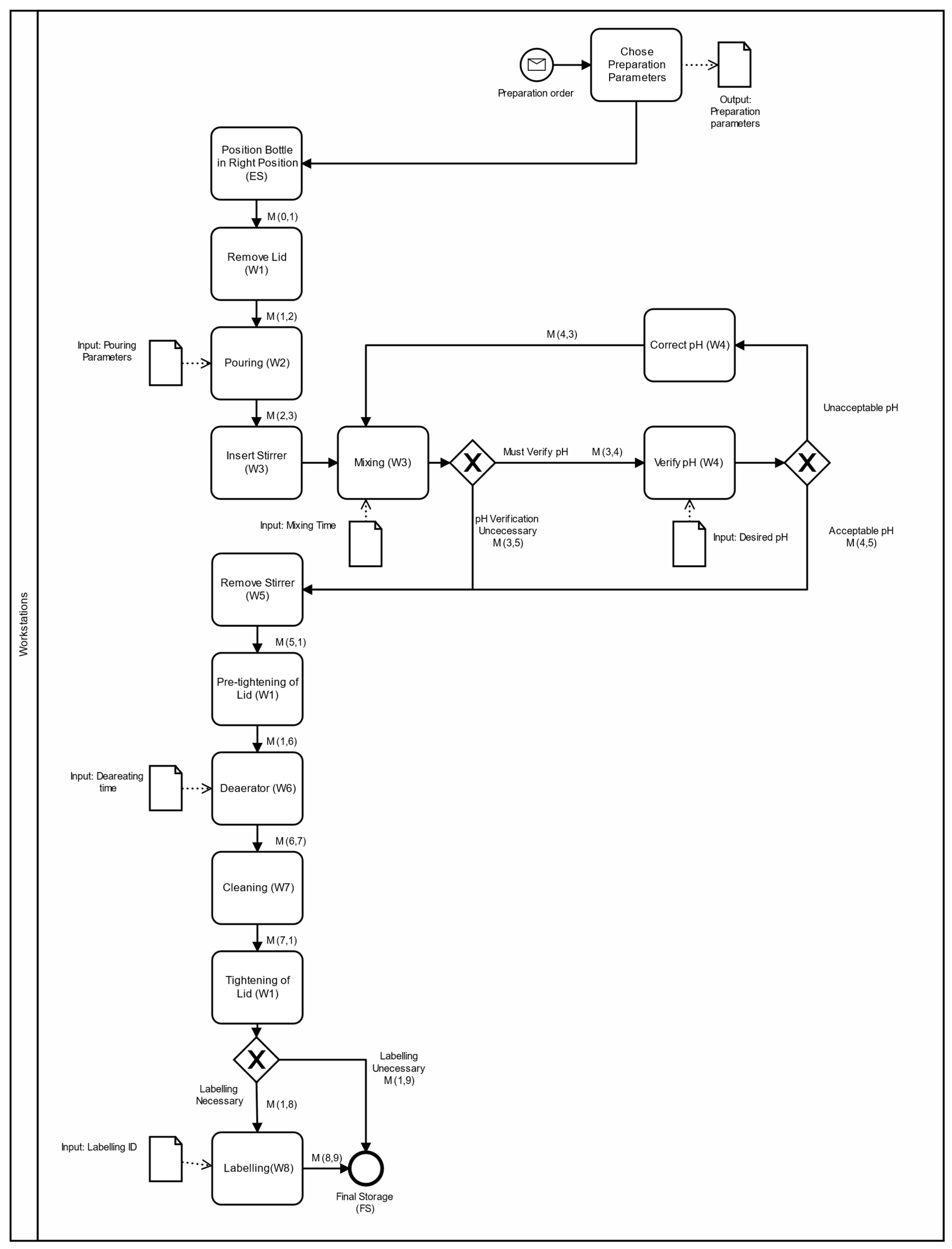
To better understand how the digital twin was developed and how the processes interact with each other, the BPM notation [36] was used to define the process workflows of our use case, summarized in Figure 5.

The industrial prototype makes liquid solutions in bottles, which can be described as jobs $J_1,J_2,\dots ,J_n$ to be scheduled in the machines W1 to W8 with the order represented in Figure 5, where each job has a specific route through the workstations depending on customer requests and real-time decisions.

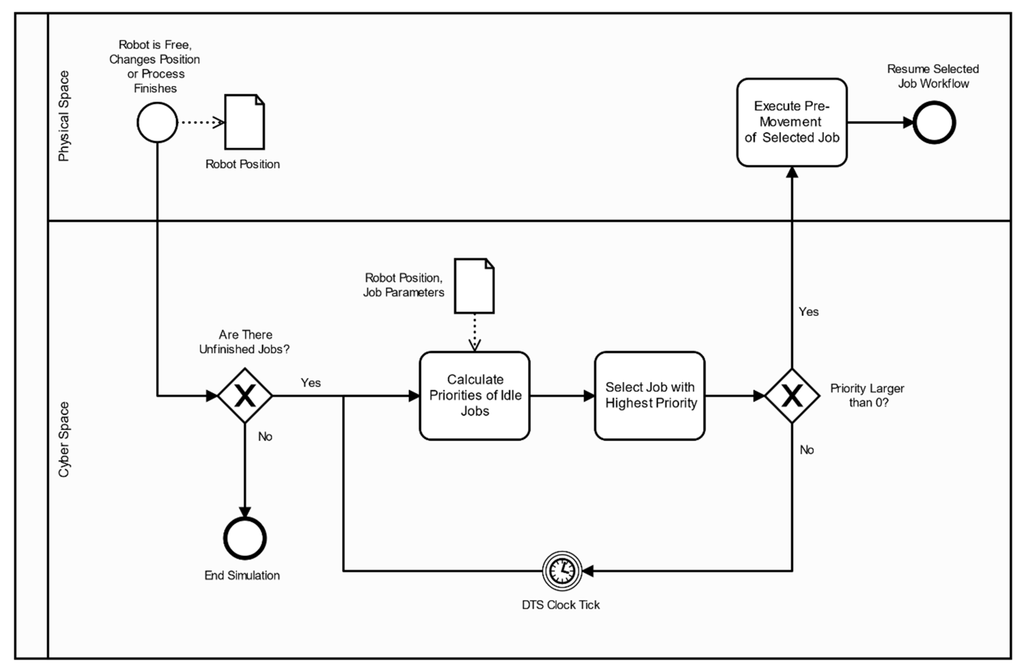
Real-time events can affect each job workflow, such as the number of iterations between W3 and W4 until the pH is correct or real-time changes in the processing time of W3 and W6. Additionally, the stochasticity associated with the random arrival of jobs is difficult to predict. These dynamic proprieties make scheduling a difficult task, as it quickly becomes obsolete, making rescheduling too frequent and ineffective. Real-time changes make reactive scheduling an option to apply in this case study (Figure 6).

In Figure 6, reactive scheduling with traditional dispatching rules such as the shortest processing time (SPT), longest processing time (LPT), and least work remaining (LWR) was employed, which defines the priority of jobs currently not being processed. According to the chosen dispatching rule, the job j with the highest priority is the next one to be processed. Priority is set to zero if the next workstation in the workflow is full or if the movement might stop the flow of tasks and result in a standstill or blockage of the system. The dispatching rule equations are presented next.

In the shortest processing time (SPT), each job has an associated priority $P_j$, with $j$as the job number and $t_{ij}$ as the processing time of operation $i$, defined as:

$$P_j=\frac{1}{t_{ij}+\epsilon }$$

(1)

If the next movement is towards the final storage (FS), $t_{ij}$ is zero and the priority is infinite. To prevent this, a small number ($\epsilon$) is utilized in the priority equation. The longest processing time (LPT) is presented in Equation (2).

$$P_j=t_{ij}+\epsilon$$

(2)

In the case of LPT, the small number ($\epsilon$) is used to distinguish the priority from zero, meaning that the job is not available. Next, the least work remaining (LWR) sums up all the processing times of a job $j$, from the current operation $c$ until the last one $r$:

$${\displaystyle \sum }_{i=c}^r(t_{ij})+\epsilon$$

(3)

Since the transportation time is long, the robotic arm movement can be relevant in scheduling decisions. Next, two heuristics based on the movement time were employed to analyze how they fare against traditional scheduling algorithms.

The shortest movement time (SMT) prioritizes jobs that are closer to the current position of the robotic arm based on the time it would take for the robot to reach the desired workstation. The priority of a job is defined by Equation (4).

$$P{i}_j=\frac{1}{M{p}_{pi}+\epsilon }$$

(4)

In Equation (4), the priority $P$ of the workstation $i$ and job $j$ is inversely proportional to $M{p}_{pi}$, which is the pre-movement time from the current location of the robot $p$ to the workstation $i$.

In the current shortest movement time (CSMT), when the robot places a bottle in a workstation, it might be beneficial to wait for the process to finish, and to transport that same bottle. CSMT employs the SMT idea for jobs currently not being processed or free jobs, and it compares the priority of these jobs, in Equation (4), with the priority of the job that the robot just transported, defined as the current priority, which is based on the processing time. The current job is defined as the job in which the robot is about to finish transporting, and its priority equation is defined as:

$$P{c}_j=\frac{1}{t_{ij}+\epsilon }$$

(5)

3.3. Discrete Event Simulation Implementation

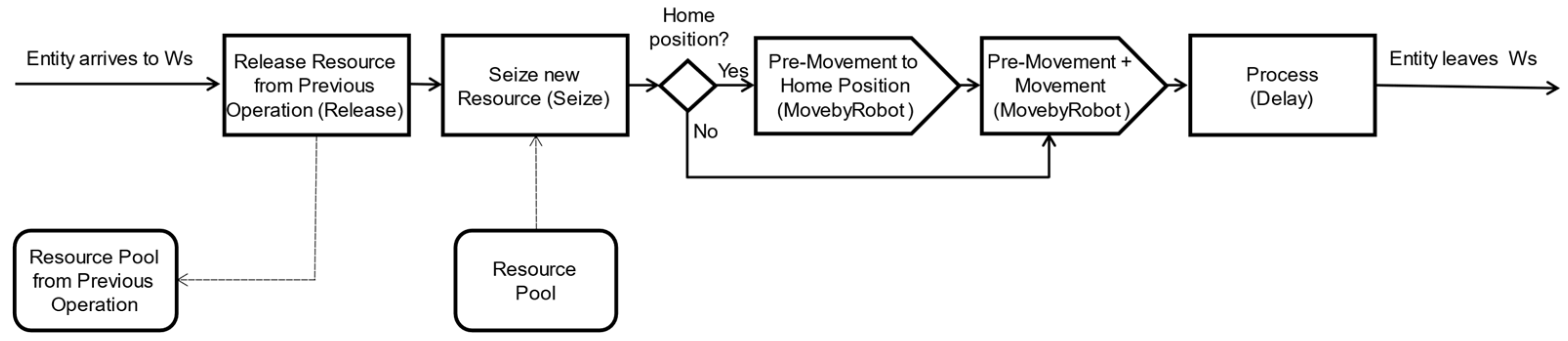
AnyLogic was used as the simulation modeling software, supporting agent-based, discrete event simulation methodologies. The simulation model was modeled as a sequence of processes corresponding to the workstations. Each process has a set of blocks such as Seize (to seize a workstation), Resource Pool (available Ws), Move by Robot (robot movement), Release (release a bottle from the workstation), and Delay (processing time), as represented in Figure 7.

In Figure 7, the home position is used for calibration and may or may not be used between robot movements between workstations.

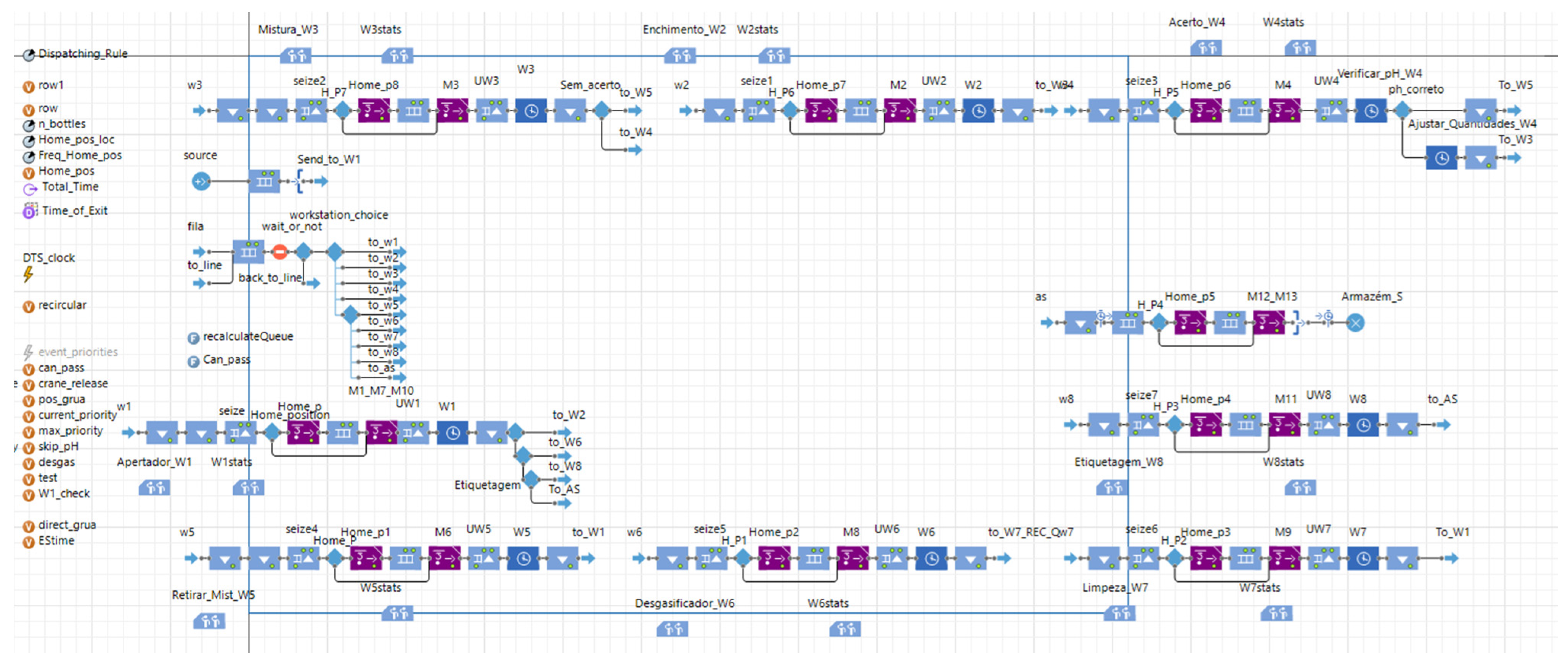
These activities can be described in AnyLogic by recurring to the process modeling library and the material handling library. A general overview of the model can be seen in Figure 8.

The chosen software also supports both 2D and 3D animation, which provides additional data to understand the model and make sure it is functioning correctly. It helps visualize the robotic arm movements and interactions with the bottles more easily while the simulation is running. In Figure 9, we can see a visualization window of the robot during a simulation run.

Concerning the information exchange from the simulation model to the real system and digital twin, the simulation model selects the best heuristic for each resource configuration based on the ongoing list of jobs and sends it to the digital twin. Additionally, the simulation model proposes a set of throughput improvements to the real system that need evaluation based on their respective investments.

4. Simulation Model

4.1. Data Processing

The processing time of each task and movement was computed from the beginning and end times taken from the digital twin.

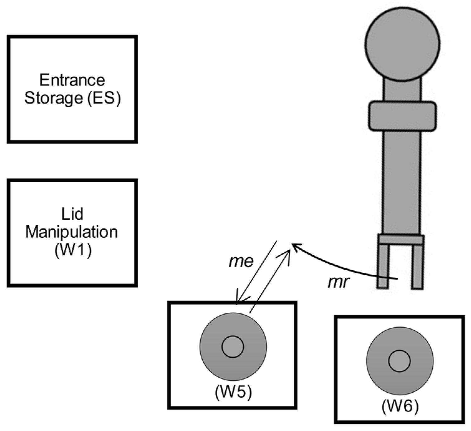
The robotic arm movement is divided into three components: the approach motion time ($ma)$, the rotational motion time ($mr)$, and the exit motion time ($me)$. These are to approach the workstation and place the bottle, to complete the rotation between workstations, and to take a bottle from a workstation, respectively. The motion of retracting the robotic arm after the approach and the exit are included in these motion times.

When switching between jobs, the pre-movement time ($M{p}_{pi})$ is employed, which consists of the rotation motion without a bottle from its current position ($p$) to the workstation where the next movement starts ($i$). Then, the robot performs the exit motion for the Ws ($i$), grabbing the bottle (Figure 10).

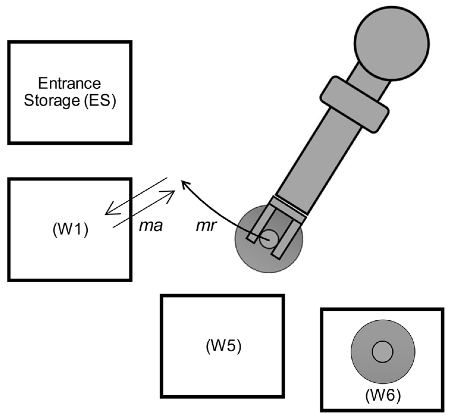
The movement time ($M_{ii,})$ consists of the rotation motion time ($mr)$ with a bottle from the workstation where the movement starts ($i$) to the next workstation ($i,$), where the robot leaves the bottle with the approach motion time ($ma)$, as shown in Figure 11.

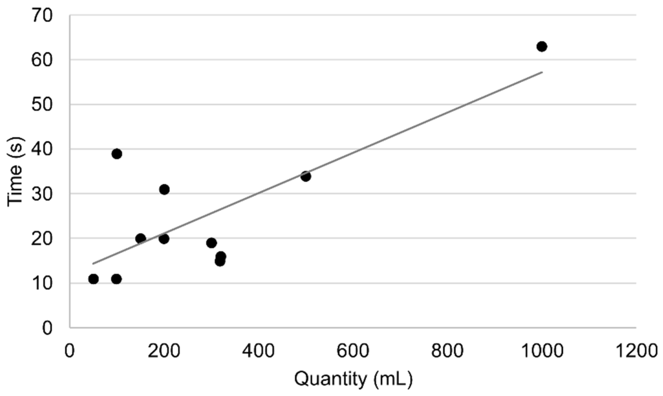
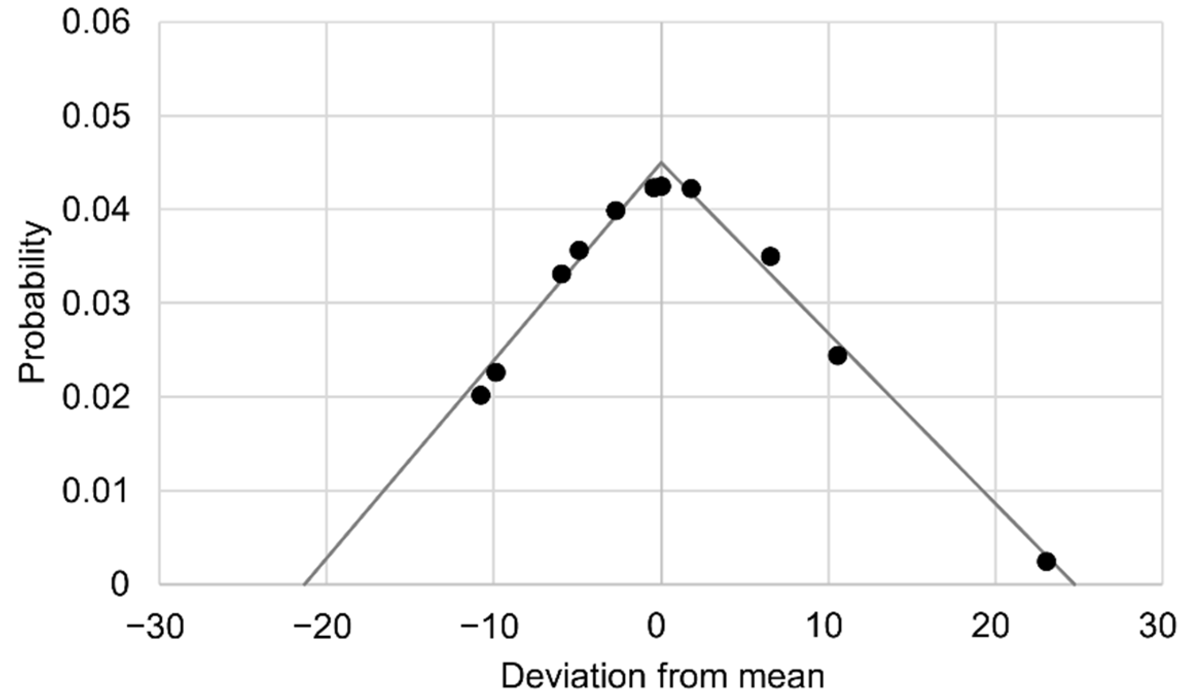
Some processes have a predictable processing time, such as removing or tightening the lid; however, there are some exceptions. In W2, bottles are filled with up to three different solutions. These can have variable quantities depending on the personalized request. Generically, the time it takes to fill the bottle depends on the amount of each liquid solution in the recipe. The quantity of liquid is measured with a scale, and the flow diminishes when the weight is close, taking longer to fill as it gets closer to the desired amount, which adds variability to the process. The time to fill a bottle was approximated using the following linear regression in Figure 12.

To emulate the high variability of the process, a probability density function $f\left(x\right)$ was applied to the resulting data based on the distance of each point to the linear regression, and a triangular fitting was computed, as represented in Figure 13.

In W3, the processing time depends on the amount of liquid filled in W2. Similarly, W6 also depends on the amount of liquid. Linear regressions and triangular distributions were also used to describe their processing times. Both processing times W3 and W6 can be changed in real time by the action of workers. Decisions such as the need for a bottle to check the pH and labeling come from the recipe. About 50% of all solution preparations need to have their pH checked. Of those, 40% need to be repeated. Regarding labeling, 70% of recipes need a label.

Regarding the generation of jobs, the simulation relied on random sampling from a list of 500 personalized jobs, following a uniform distribution. The input data and list of recipes, taken from historical data, include the processing times for each workstation, as presented in

Table 2. Recipe processing times for each workstation, in seconds. Examples.

JobID	W1	W2	W3	W4	W5	W1	W6	W7	W1	W8
1	14.5	58.4	377.1	10.0	14.0	6.5	150.0	25.5	7.5	0.0
2	14.5	74.0	286.3	0.0	14.0	6.5	300.0	25.5	7.5	27.0

.

Process variations, emulated by the triangular distributions, were embedded in the model in addition to these values to simulate the stochastic conditions. Regarding W4, when a job must do a pH check from the recipe, the probability of it going again follows a Poisson distribution. The processing times for each movement are detailed in Section 4.2.

4.2. Validation

As mentioned earlier, the manufacturing system was being improved to run multiple jobs simultaneously. Therefore, some extrapolations had to be done to obtain all the possible combinations of movements between workstations that were missing in the original data. For simplification purposes, the robotic arm movement between workstations was modeled as a crane with only rotation motion instead of 6 degrees of freedom.

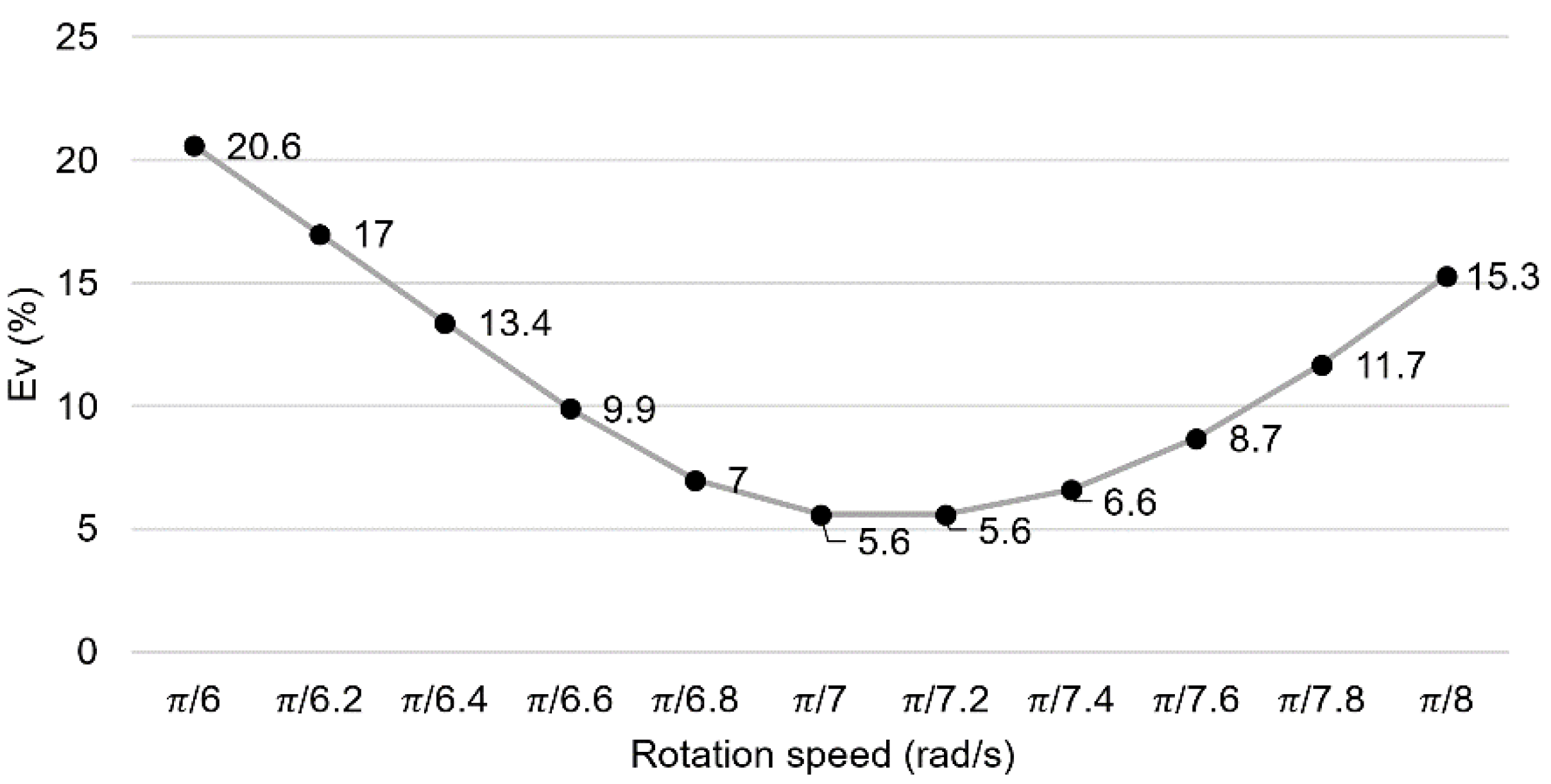
Naturally, the average rotation speed $v$ varied slightly depending on the movement due to being in a tridimensional space. An acceptable rotation motion speed for the robot, with the rotation time ($mr$), needed to be chosen for calibration of the model.

The verification was done by analyzing simulation runs, removing the stochasticity and comparing those with known actual values. The goal was to test the total processing time of simulations when fed the same input data as in the real counterpart. For calibration, different values of rotation speed were tested to see which value more closely emulated the real counterpart. Rotation speeds from 3 rad/s to 4 rad/s were tested, and the relative approximation error $E_{iv}$ was computed at the end of each operation ($i$) in Equation (6).

$$E_{iv}=\frac{\left|T{s}_{iv}-T{r}_i\right|}{T{r}_{iv}}\times 100$$

(6)

where $T{s}_i$ is the simulation time at which process $i$ finishes for rotation velocity of $v$, and $T{r}_i$ the real-time at which process $i$ finishes. The accumulated relative approximation error $E_v$of all operations ($r$) was used as a measure of performance, with the results presented in Figure 14 [37].

$$E_v={\displaystyle \sum }_{i=1}^r\left(\frac{\left|T{s}_{iv}-T{r}_i\right|}{T{r}_i}\times 100\right)$$

(7)

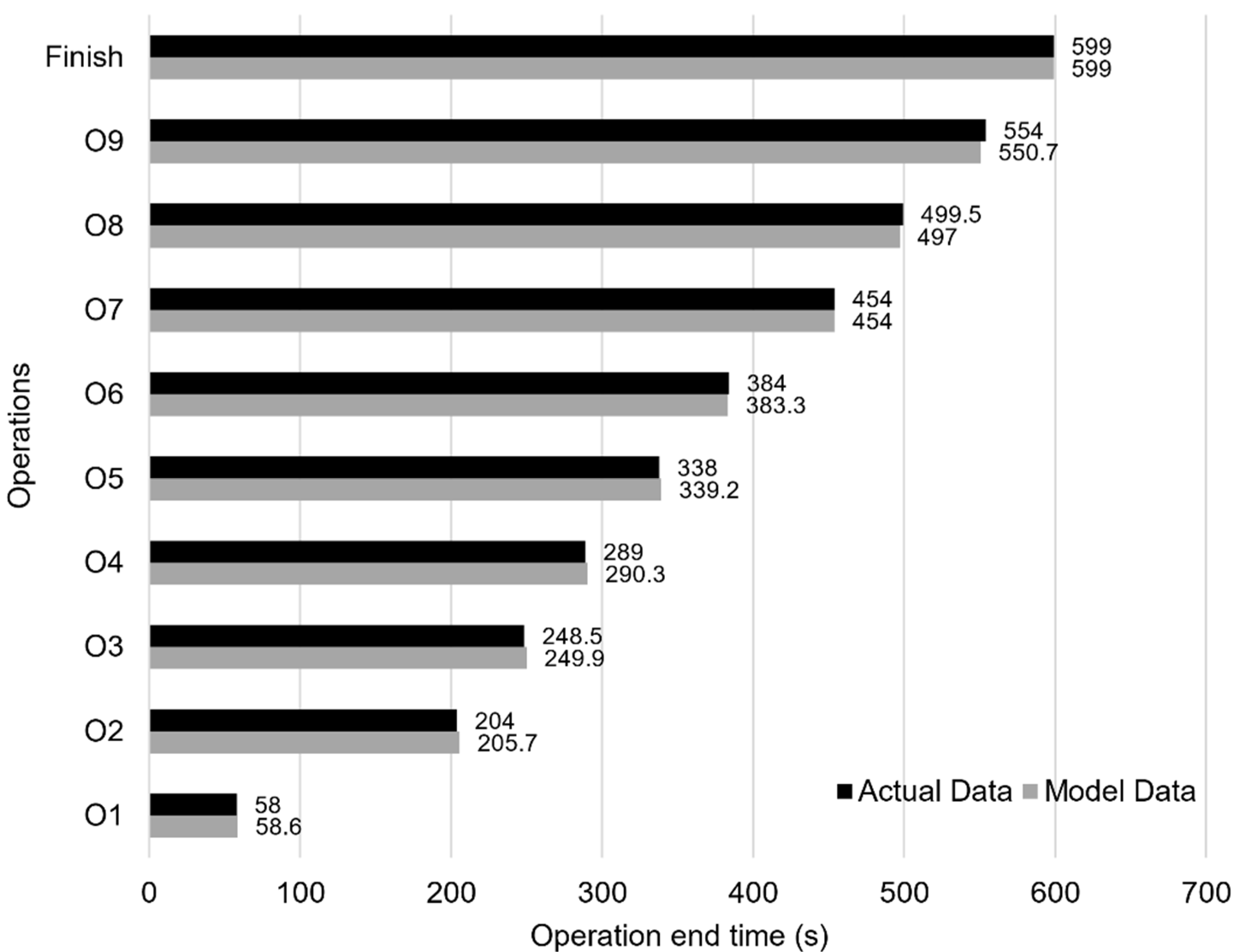
In Figure 14, π/7.2 rad/s is the value that ensured the smaller accumulated error of 5.6%, and so it was the speed chosen for calibration and validation. The 5.6% is the average error between the time it took to complete actual recipes in the real manufacturing system against their simulated counterpart when considering the robotic arm modeled as a crane with a rotation speed of π/7.2 rad/s. Figure 15 compares the completion time between validation and the digital twin.

Although this approximation is not as valuable as having real data regarding all the movements, it can describe the movement times for the existing system with enough accuracy. Both the digital twin and the discrete event simulation model were fed with tables containing the rotation ($m{r}_{ii,}$), pre-movement ($M{p}_{pi}$), and movement times ($M_{ii,}$) with all the possible movements.

In situations where no information is available, time studies can be conducted. Recorded videos and stopwatches are common strategies used to retrieve the processing time from repetitive or cyclic tasks and when there is variability in the jobs [38,39]. According to Magagnotti et al. [40], a comprehensive time study consists of the following steps: study goal, experimental design, measurements in the field, and data analysis.

5. Results and Analysis

After the model validation, the next step was to do simulation runs or iterations with multiple bottles and a variety of different parameters to discover which decisions reduced the makespan and increased the utilization of the equipment. Different measures of performance were used.

Makespan ($T$): time to process all the jobs, or total time.

Resource utilization ($U_w$): measures the utilization of a workstation or the robot, and is the relationship between the total working time of a resource ($T{u}_W$) and the makespan (Equation (8)):

$$U_w=\frac{T{u}_w}{T}$$

(8)

Resource occupation ($Ro$): measures the occupation of a workstation, that is, the percentage of the time each workstation has a bottle, independent of the working time, and is the relationship between the occupation time of a resource ($T{o}_w$) and the makespan (Equation (9)):

$$O_w=\frac{T{o}_w}{T}$$

(9)

Performance improvement ($I$): also called makespan reduction or reduction in total completion time. The goal is to compare the makespan of different iterations and measure the effect of parameter changes, with $T_p$ as the makespan of the iteration used as a comparison term (Equation (10)).

$$I=\left(1-\frac{T}{T_p}\right)\ast 100$$

(10)

5.1. Multiple Jobs

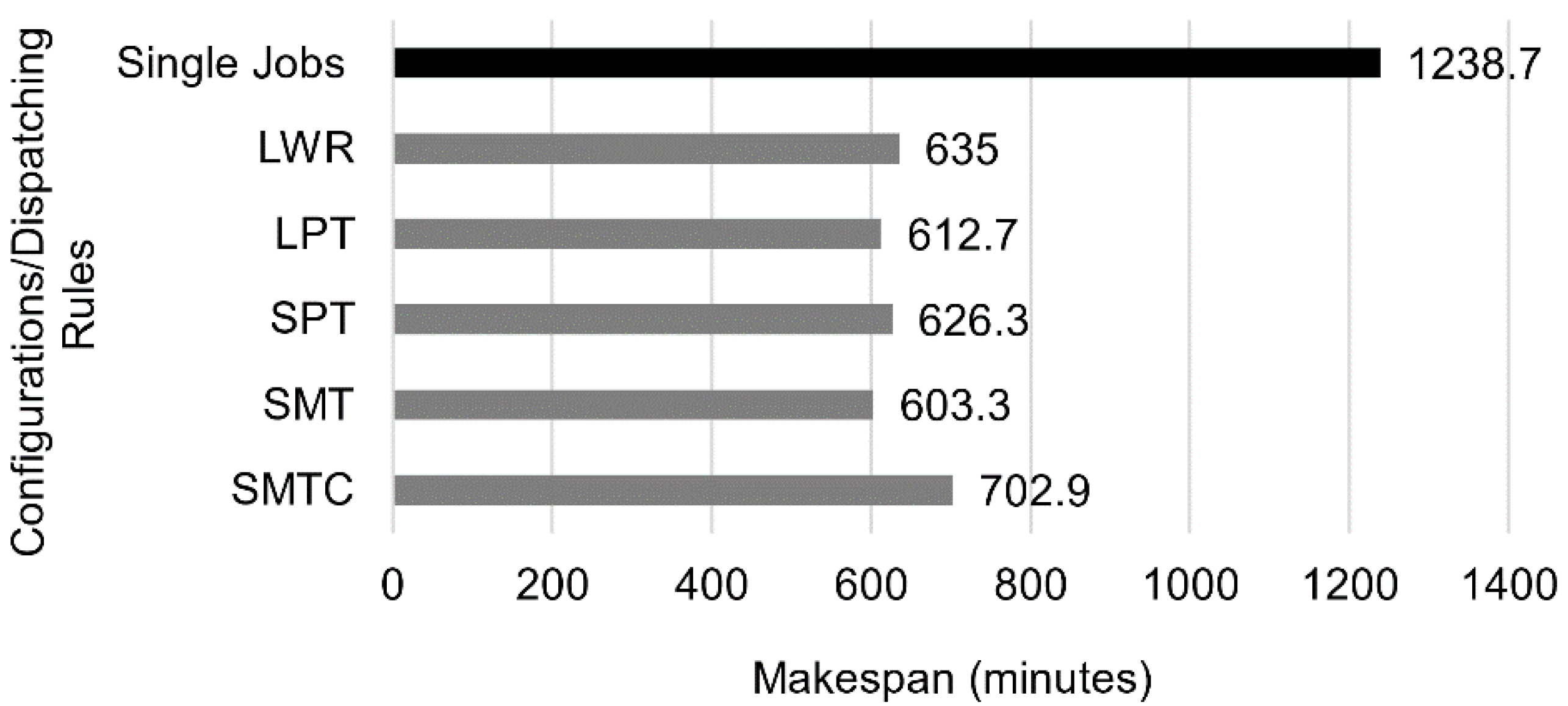
The system currently only supports one job (single jobs) at a time. The new job is only processed when the last one is completed. As said in the introduction, one of the goals of this paper was to see the effect of multiple jobs on the completion time, with different heuristics. To do so, an iteration with single jobs was compared with multiple jobs with the dispatching rules referred to in Section 3. A total of 50 jobs were used as inputs to the simulation model. To achieve statistical significance, we computed the mean value of 1000 iterations for each scenario. We chose 1000 iterations, as the error was below 1% with a confidence interval of 95%. The time to complete 50 bottles in 1000 iterations was around 3 min. The reaction time of the dispatching rules was virtually instantaneous. In Figure 16, we can see the makespan comparison of single jobs against multiple jobs, considering different heuristics.

Combining multiple jobs with the SMT dispatching rule led to the best results, reducing the overall completion time by 51.3%. This result shows how imperative it is to allow multiple jobs to run in the system, even without adding new resources.

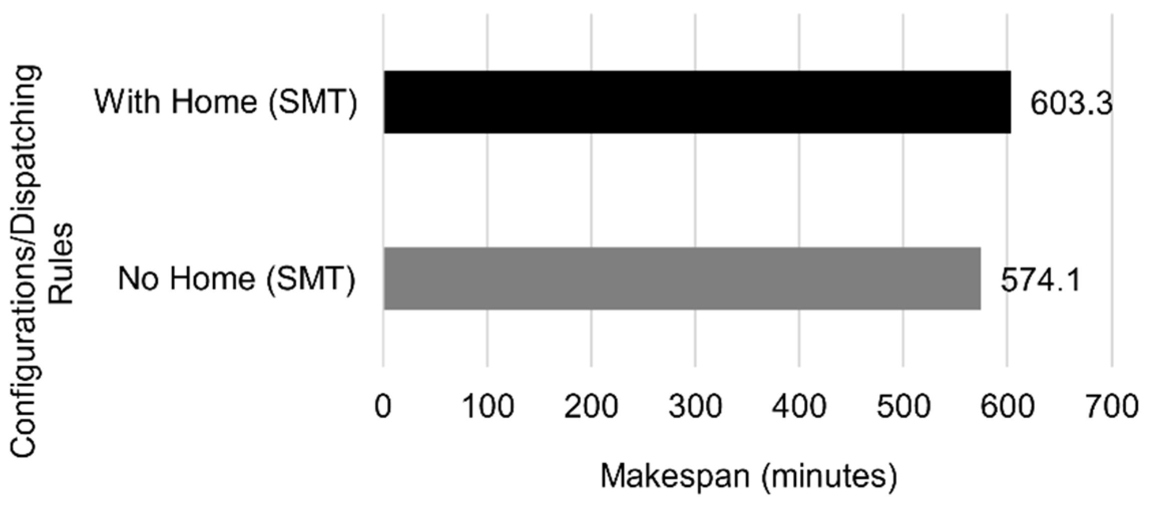
5.2. Home Position

The robotic arm needed to go to the home position multiple times to avoid accumulating errors. However, removing that need, the robot occupation was reduced and the performance was improved, as seen in Figure 17.

Avoiding the home position led to a reduction in the makespan of 4.8%. This reduction was achieved by only letting the system go to the home position when the robotic arm was idle.

5.3. Resource Allocation

Tables with resource utilization, resource occupation, and performance improvement were analyzed to understand which workstations should have parallel machines.

Table 3. Utilization of each resource in the no home (SMT), single machine configuration.

Resource	Utilization (%)
Robot	51.1
W1	8.3
W2	16.7
W3	78.8
W4	3.1
W5	4.1
W6	43.7
W7	7.4
W8	1.9

shows information relative to workstation and robot utilization for the model with single machines for the SMT dispatching rule, as it was the one with the lowest makespan.

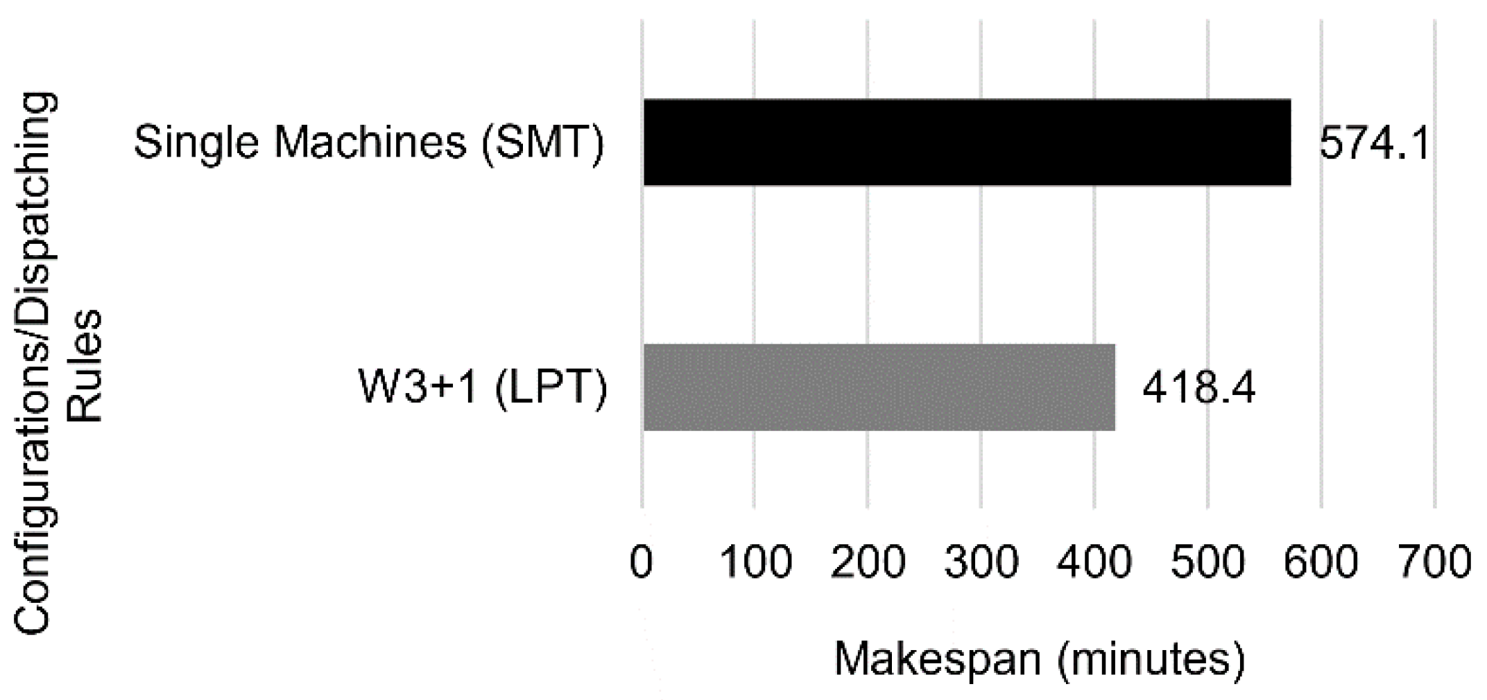
W3 had the largest utilization and occupation rate, followed by W2 and W4, implying that the bottles at these Ws spent most of the time waiting, which indicates a possible bottleneck at W3. Therefore, the first step was adding an extra W3 (Figure 18).

Adding a parallel W3 yielded an increase in performance of about 27.1% using the best performing dispatching rule with single machines, meaning W3 was a bottleneck. Applying this change in the real counterpart proved effective, with the LPT algorithm being the most effective for the configuration. In this new configuration, the W3 might still have been a bottleneck as its occupation ratio was still high. The W6 might also have been another possible bottleneck. W1 could also have been another bottleneck, because each job went through it three times, making the consideration of an extra parallel W1 a possible improvement to the system. 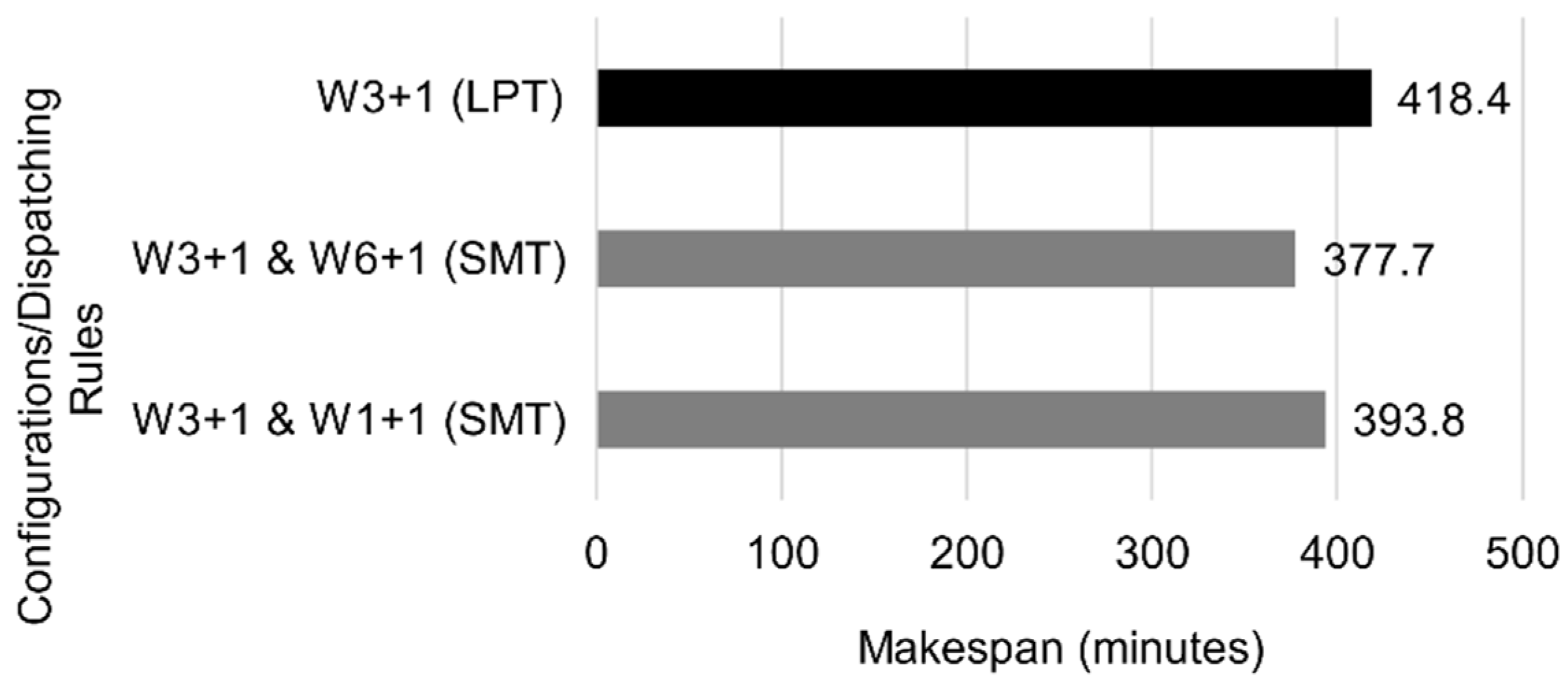Figure 19 makes further comparisons considering two W3s, W6s, and W1s.

Following the simulation model results, an additional machine in the W6 with two W3s further decreased the makespan by about 9.7%. Alternatively, adding an extra W1 when already having two W3s resulted in a performance increase of 5.9%. The viability of adding a new W3 or W6 depends on the cost of the equipment.

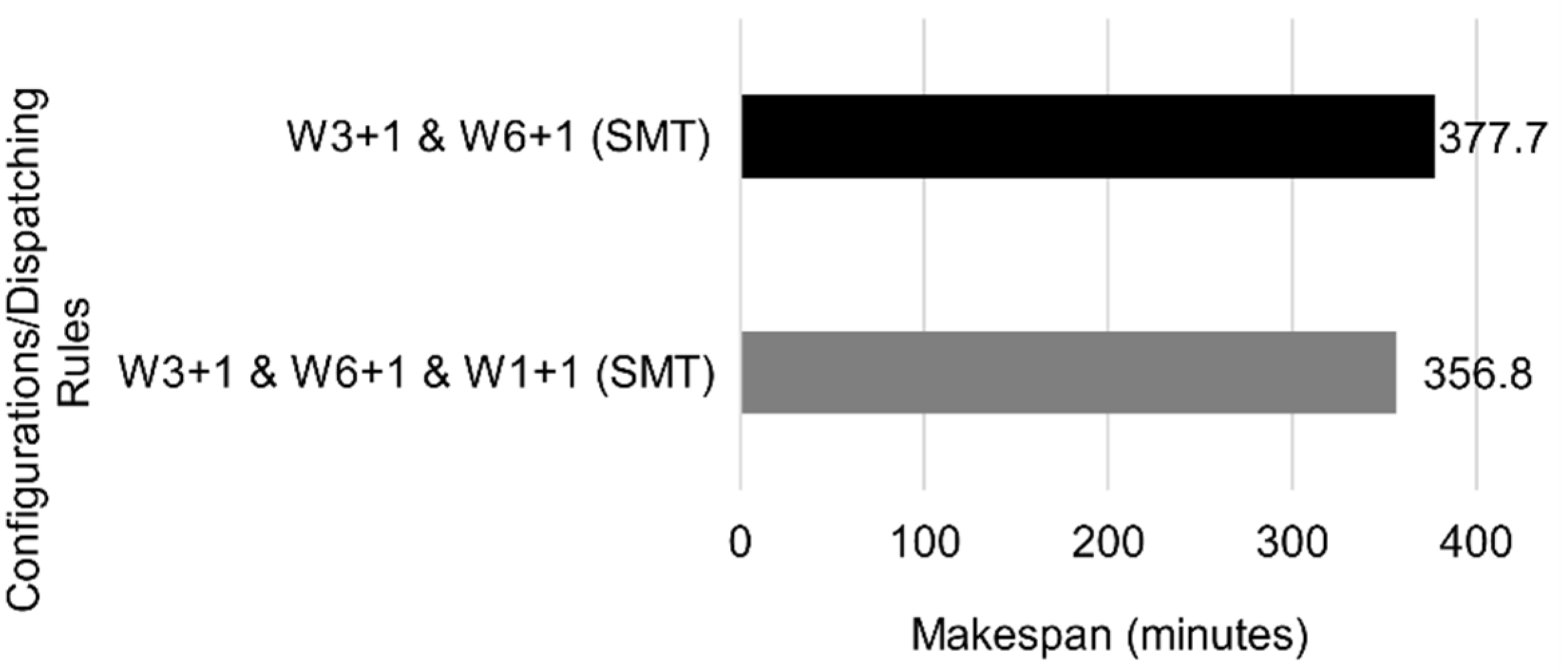
Because W3 still possessed the highest utilization, it restricted the workflow. W6 had the second-highest utilization. W1 appeared to restrict the flow of tasks, as W5 had a low occupation ratio since each job needed to go through W1. Having a single machine might create a choke point. Because the combination of an extra parallel W3 and W6 had the lowest makespan for most dispatching rules, it was used as a comparison term to other configurations (see Figure 20).

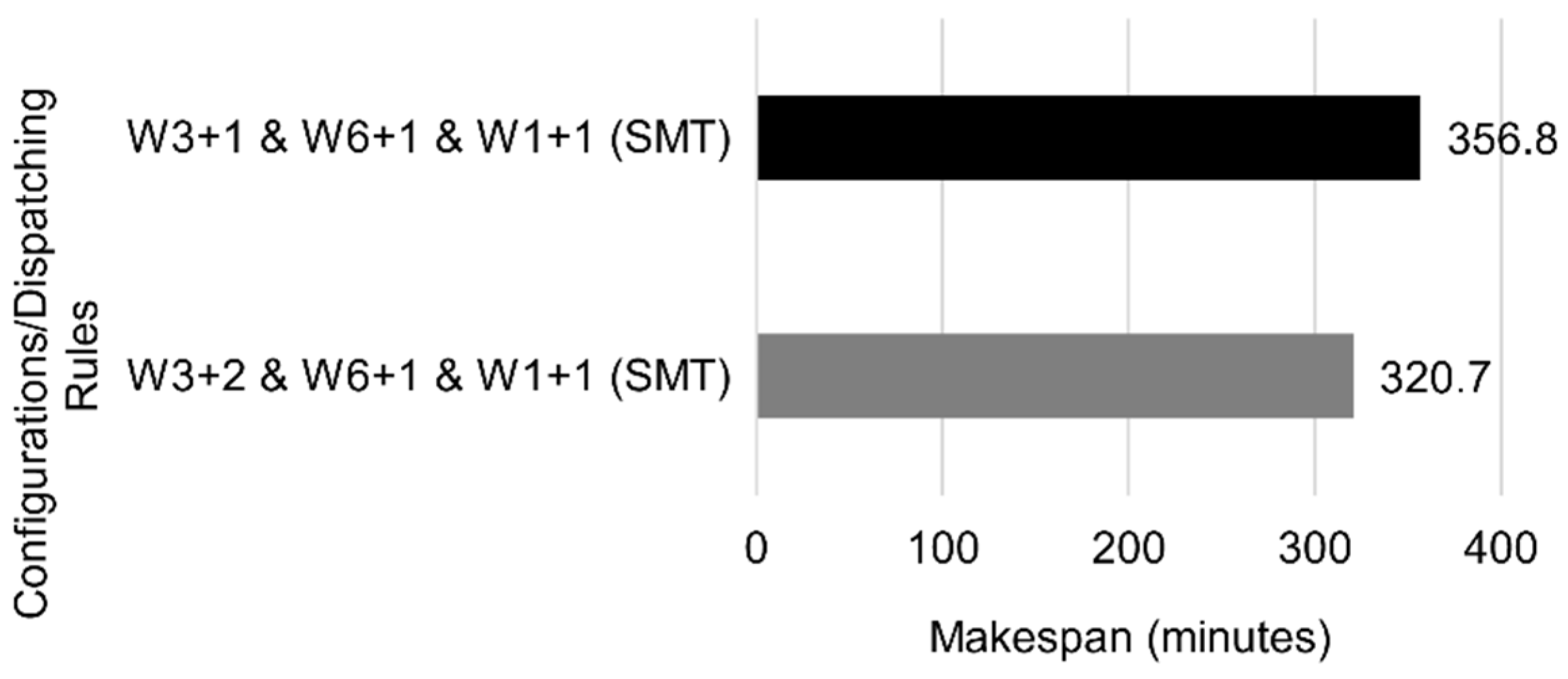
Including an extra W1 in the configuration already possessing two W3s and W6s yielded the highest reduction in makespan, of 5.5% (Figure 21).

Adding an extra W3 further reduced the makespan by 10.1%. Other additions were tested using this configuration as a reference; however, the makespan did not decrease more than 2%, so adding more Ws did not yield much better results.

In this setup, the robot was used most of the time (92.6%). Although the workstations still had an overall low utilization, increasing the number of parallel machines no longer yielded reductions in makespan larger than 2%. Additionally, the fact that the SMT rule, which relates to the robotic arm speed, was performing better than other dispatching rules makes a study on the robot movement speed a relevant topic.

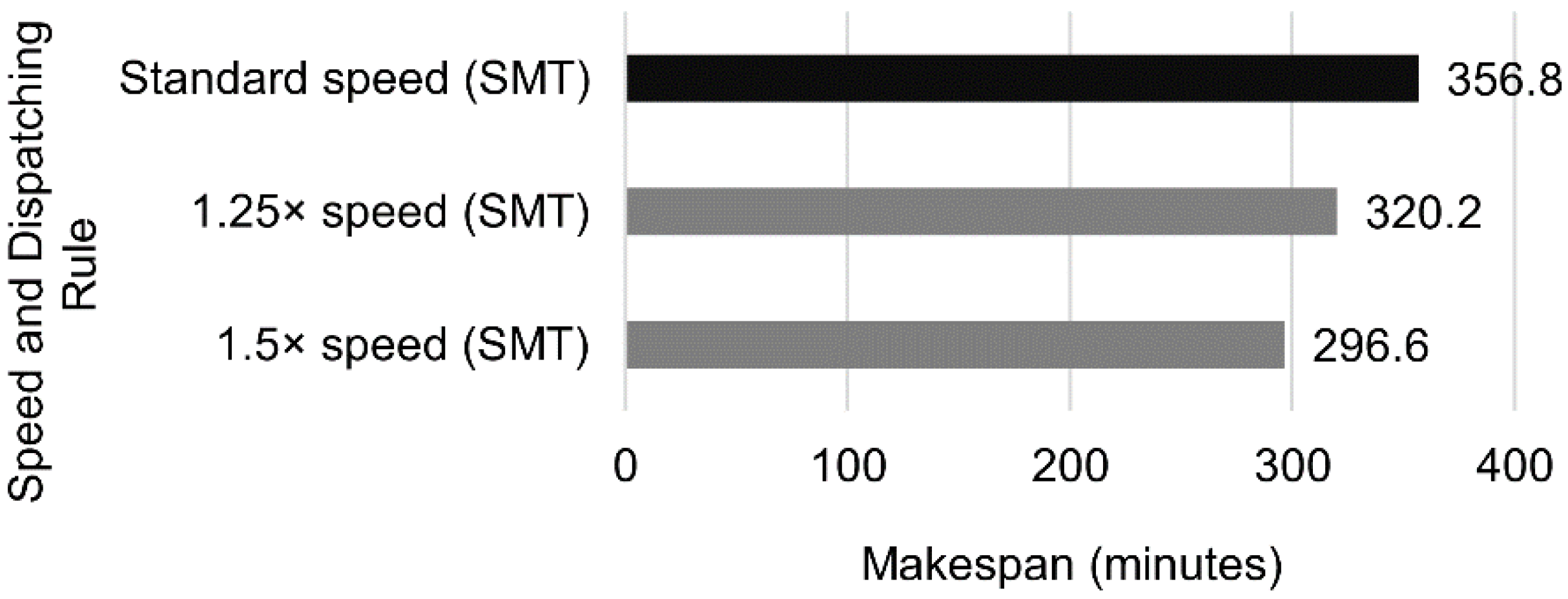
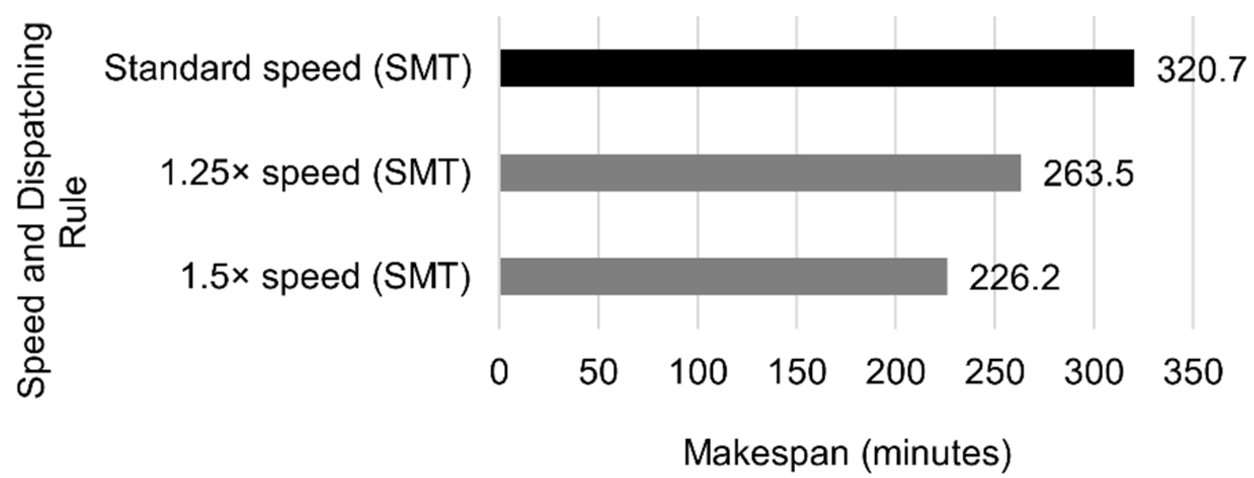
5.4. Robot Speed

The robot currently works at a conservative speed for security reasons, but it can be increased. Previous configurations with the highest impact on the makespan were accelerated by 1.25 and 1.5, with the following results as shown in Figure 22.

Standard configuration:

Using two W3s leads to the results in Figure 23:

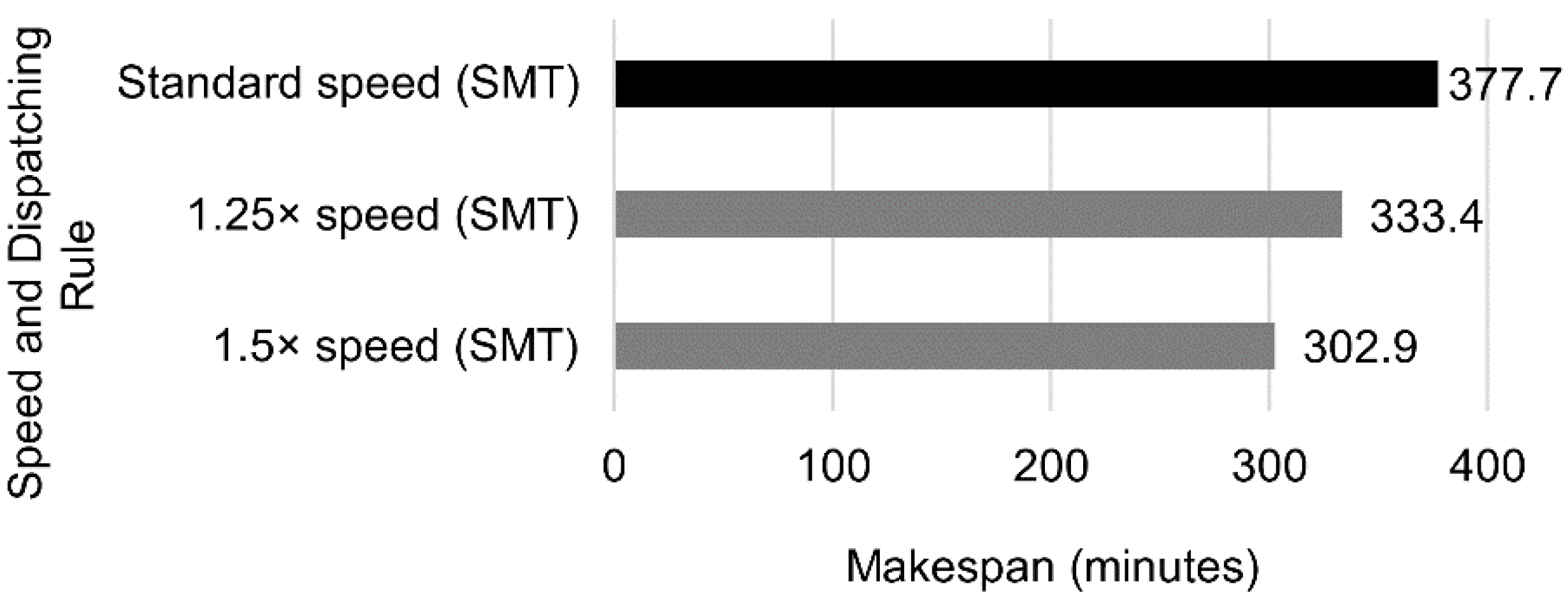
Using two W3s and W6s leads to the results in Figure 24:

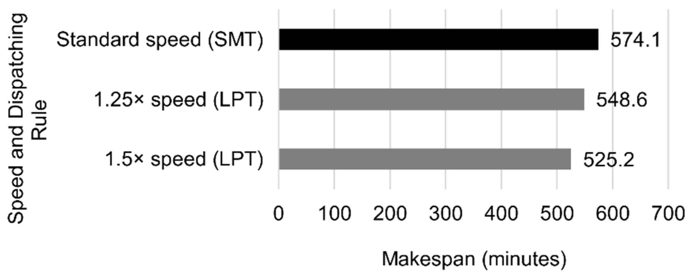
Using two W3s, W6s, and W1s leads to the results in Figure 25:

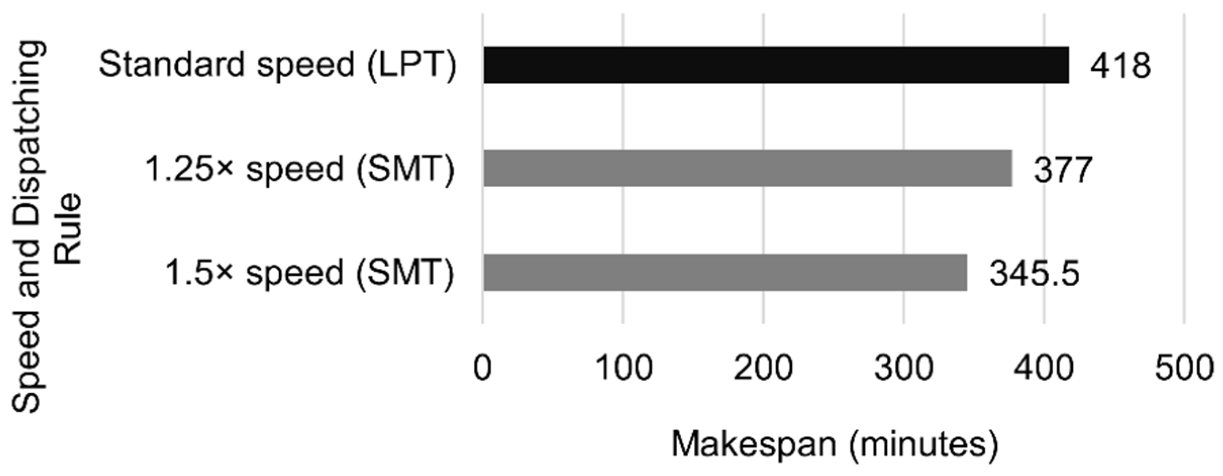
Using three W3s and two W6s and W1s leads to the results in Figure 26:

Increasing the robot velocity did not reduce the completion time when there was only one machine per workstation. However, in the configurations with several machines, increasing the speed by 25% and 50% resulted in makespan reductions of 9.8% and 20.5%, respectively.

Combining an increase in robot speed with adding specific workstations can be considered the best option. Choosing the right combination depends on the cost and feasibility of each change—information that the authors do not possess.

6. Conclusions and Future Work

This paper proposes a digital twin to simulate a manufacturing system (to prepare solutions) affected by personalized production in real time. The flexible manufacturing system uses a robotic arm as a transportation element between workstations, allowing for multiple jobs simultaneously in the system. The digital twin architecture developed and implemented can handle various customer requests, robot movement speeds, and different combinations of machines in the workstations. It utilizes reactive scheduling with five different heuristics: SPT, LPT, LWR, SMT, and CSMT. The conducted forecasts considering different scenarios proved that using multiple jobs in parallel with an SMT dispatching rule reduced the makespan by 51.3% compared to only having the robot doing one job at a time. Experiments with additional parallel identical machines were conducted, proving that the single addition that proved most effective was adding one W3, which decreased the overall completion time by 27%. The robotic arm speed was also a topic of analysis, proving beneficial when parallel machines were added in the configuration with two extra W3s and one extra W6 and W1 when increasing its velocity by 50%, yielding a reduction in makespan of 29.5% compared to standard speed. Combining a 50% increase in speed with the configuration W3 + 2, W6 + 1, and W1 + 1 resulted in a makespan reduction of 82% compared with the base configuration with single tasks and single machines.

Between all heuristics, SMT proved to be the most effective in reducing makespan, with the LPT outperforming the SMT in a few configurations.

Overall, the objective of developing a digital twin capable of making real-time decisions was achieved by utilizing completely reactive scheduling. The ability to do forecasts with different dispatching rules, various machine configurations, and robot speed, with access to a visualization window for a more intuitive understanding of the model, gives stakeholders more information on where the system can be improved.

Future work will focus on improving the scheduling algorithm as follows:

• Study dispatching rules that reduce the overall transportation time to reduce the makespan.
• Improve the CSMT dispatching rule. One of the issues with this dispatching rule is that when the robot waits for long processes, it keeps waiting until the task finishes, independently of any jobs becoming available. An improved CSMT dispatching rule could take advantage of the DTS clock to run checks on the system, triggering the decision processes and interrupting the wait if another job has higher priority.

Furthermore, the operator can have the option of making scheduling decisions, having the ability to override DT scheduling decisions and creating a more human-centric environment, which is included in the goals of Industry 5.0.