Abstract
Indonesia is a maritime country that has vast coastal resources and biodiversity. To support the Indonesian maritime program, a topography mapping tool is needed. The ideal topography mapping tool is the Unmanned Surface Vehicle (USV). This paper proposes the design, manufacture, and development of an affordable autonomous USV. The USV which is composed of thruster and rudder is quite complicated to build. This study employs rudderless and double thrusters as the main actuators. PID compensator is utilized as the feedback control for the autonomous USV. Energy consumption is measured when the USV is in autonomous mode. The Dynamics model of USV was implemented to study the roll stability of the proposed USV. Open-source Mission Planner software was selected as the Ground Control Station (GCS) software. Performance tests were carried out by providing the USV with an autonomous mission to follow a specific trajectory. The results showed that the developed USV was able to complete autonomous mission with relatively small errors, making it suitable for underwater topography mapping.
1. Introduction
Indonesia is a country in Southeast Asia and Oceania located between the Indian and Pacific oceans. It consists of over seventeen thousand islands, including Sumatra, Java, Sulawesi, and parts of Borneo and New Guinea of which three-quarters of its territory is a sea. It is reasonable that Indonesia has enormous coastal resources and biodiversity. To support Indonesia’s maritime program to strengthen the identity as a maritime country, and the economic development of maritime and marine, the government require the tools to carry out bathymetry mapping, a mapping to monitor the topographical condition of the seabed, which is beneficial for determining safe shipping lanes, planning coastal buildings, planning underwater pipelines, planning offshore drilling, and detecting Tsunamis.
Suitable for these duties is the Unmanned Surface Vehicle (USV), which is an autonomous boat operated on the surface of the water without a crew, and which surveys the area autonomously in line with what has been programmed by the operator into the module. Previously, unmanned vehicles, such as Unmanned Aerial Vehicles (UAV) and Unmanned Ground Vehicles (UGV)/mobile robots, had become popular research topics in developing countries because of their versatility, and ease of development. For example, the development of an ornithopter-shaped UAV controlled by a radio control system [1], the development of a UAV embedded with a disinfectant spraying system to break the chain of the COVID-19 virus [2], and fuzzy-based fault-tolerant control for an omnidirectional mobile robot with four mecanum wheels [3].
The Unmanned Surface Vehicle is the same as others being controlled automatically by giving commands from the Ground Control Station (GCS). Prior to issuing a command, GCS receives data from the sensors, which are integrated into the USV, for instance Global Positioning System (GPS), Compass, and Inertial Measurement Unit (IMU). These sensors are powerful as long as there is no interference with magnetic disturbance [4] and they are calibrated regularly to generate accurate data to achieve the desired position.
In its application, USV incorporated with various sensors can directly map the topography of water and operate for a long period without polluting the water. USV is very potential to be used in surveillance missions in certain areas such as: monitoring certain areas or observing events that are not safe for humans, monitoring foreign ships around Indonesia that are likely to commit illegal fishing. USV can also be used for monitoring and data retrieval missions for instance monitoring seamount activity, mapping marine resources, and capturing offshore data [5]. Because USVs are relatively small in size, this makes them particularly suitable for operation in areas that are difficult to access (dams, rivers, shallow waters, canals, etc.).
USV operates in a more environmentally friendly way and can be used in hazardous operations. Compared to the Manned Surface Vehicle, a USV can reduce manufacturing and operational costs. Currently, the USVs that have been developed can produce energy to supply their power. The power can be obtained from solar radiation, wind gusts, and ocean waves. By using this energy, the USV can be operated for an extended period and at a minimum cost [6].
In the laboratory scale, certain studies associated with Unmanned Surface Vehicle have been conducted for example the simulation of autonomous boat dynamic model [7] and experimental study of autonomous boat aerodynamics [8] by Diponegoro University researchers. USV trends and challenges nowadays have been revealed by Barrera et al. [9].
Meanwhile, in its application, there were several research concerns with USVs. The development of USVs for nearly 15 years is introduced by Manley et al. [10]. Mingxi et al. employed the structure of catamaran USV aimed for estuary research; they applied Robotics Operating System (ROS) installed into Jetson Nano [11] which was also applied by Bae J. et al. for sediment sampling [12]. Iovino et al. from Cranfield University to experimental testing of a path manager [13]. While Mou et al. introduced an intelligent navigation algorithm to improve motion control and path following of the USV [14]. Sutton et al. conducted the adaptive non-linear control for the USV [15], and more sophisticated, robust control with Fuzzy Logic guidance is applied by Aguilar et al. for improving the precision of USV maneuvering [16]. Marchel et al. adopted a high precision Global Navigation Satellite System (GNSS) Real-Time Kinematic (RTK) to evaluate steering precision [17]. Even the Nonlinear Predictive Controller (NMPC) based on Convolutional Neural Network (CNN), and Ant Colony Optimizer (ACO) is proposed by Zhao et al. from Wuhan University of Technology [18].
According to those works, in most research, to develop a reliable USV that follow the command autonomously, a sophisticated controller, such as a non-linear, Fuzzy Logic control, and complex algorithm for path following design is needed, several researchers also propose the Internet of Things (IoT) concept to bridge the communication between the USV and Ground Control Station (GCS). Furthermore, expensive hardware to support the USV is also necessary. For these reasons, the development of USV is exceptionally not affordable and not prevalent to be studied in undeveloped countries. However, in this research, the traditional controller (PID combined Feed Forward) integrated to a simple algorithm, applied in affordable hardware, and using an open-source ground control station is implemented.
The mechanical structure of a USV, which is composed of a thruster and rudder, is quite complicated to build. The rudder frequently uses plastic as its primary material, which can be easily damaged by the wear of gear during the steering process. The energy conversion rate of the rudderless USV is higher than USV with rudder [19]. This study employs rudderless and double thrusters as the main actuators. The USV velocity can be controlled by increasing or decreasing the speed thrusters, while the steering of the USV is generated from the differential thrust control from the left and right thrusters.
2. Equation of Motion of the Proposed USV
In general, the study of the USV motion model is divided into two parts: kinematics, which threaten only geometrical aspects of motion, and dynamics, which is the analysis of the forces causing the motion [19]. Moreover, this section is divided into subheadings as it should provide a concise description of the experimental results. To derive the kinematics and dynamics equation of USV, the model is assumed to have horizontal symmetry.
2.1. Kinematics of USV
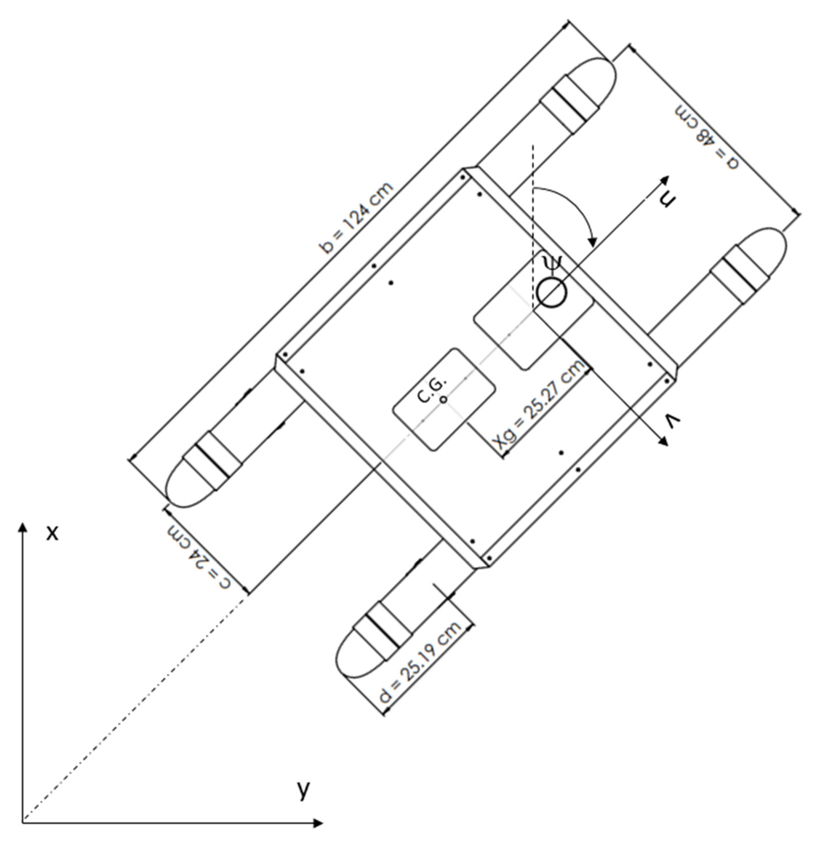
The USV is modeled as a 3 DOF system (x, y, and r axes (x, y, and r axes) [20]. The USV movements in heave (w), roll (p), and pitch (q) directions are presumed to be relatively small; therefore they can be ignored. The USV kinematics is described in two terms of reference coordinates, namely the USV frame of reference (u, v, w) and the Earth frame of reference (x, y, z). The free body diagram of this model is shown in Figure 1.
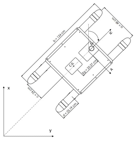
Figure 1.
Free Body Diagram (a = nose to nose distance, b = USV length, c = thruster to center of gravity horizontal distance, d = thruster to nose tip distance, xg = centre of gravity distance to USV frame of reference).
The standard notation used to define 3 DOF models in this study, based on the SNAME notation 1950 [21], is shown in Table 1.

Table 1.
Standard notation of USV motion.
To transform the equation from the USV frame of reference to the Earth frame of reference, the kinematics equation is revealed in Equation (1).
where = is the position (x, y) and yaw () of USV in the Earth frame of reference while = describe linear velocity in x, y-direction, and angular velocity in yaw () direction. is defined as the transformation matrix as shown in Equation (2).
V = is interpreted as linear velocity (u, v direction) and angular velocity (r direction) in the USV frame of reference or body coordinate system. Hence, The USV kinematics equation is given by Equations (3)–(7)
2.2. Dynamics of USV
To model the dynamics equation, it is necessary to analyze the force of the USV. USV’s dynamics model is based on Fossen’s model [22]. In simplifying the analysis, the USV is assumed as a rigid body. The dynamics equation of the USV is modelled in the form of a matrix, which is represented as
M is defined as mass matrix, C(V) represents centripetal and Coriolis matrix, and D(V) is linear drag matrix. The effect of non-linear drag is ignored as the velocity is relatively slow [17]. Meanwhile, is input forces and moments generated by the thrusters. and are external forces or moments caused by the wind and the wave, respectively. The matrix M, C(V), D(V), and are expressed as Equations (9)–(12).
and effect could be neglected because USV is sailing in calm water and a breeze environment. As a result, the effects of waves and wind (environmental disturbance) may be ignored (research was conducted at the Military Camp’s Swimming Pool in Semarang City, Indonesia). The sway force emerging from yaw rotation () and the yaw moment caused by the acceleration in the sway direction () are remarkably smaller than the inertial and additional mass terms [19]. The USV center of gravity is parallel to the USV frame of reference coordinate in the horizontal direction, thus = 0.
Then, , thrust force by thruster 1, and , thruster 2 force, are outlined as
where, F0 is defined as the total thrust force, and δ is defined as the differential thrust force between thrusters where the magnitude of δ affects the rotational speed of the yaw and the heading of USV.
The dynamics model is reduced to Equations (15)–(18) when these assumptions are applied.
, , and are additional mass when USV moves in direction u, v, and r. is the moment of inertia towards the z-axis. , , and are the sum of linear drag force coefficients when USV sails in the translational direction (u, v) and rotational direction (r), and if they are multiplied by the linear velocity (u, v) and rotational velocity (r), they become the sum of linear drag force that work in their own direction. is that in rotational direction (r). The expanded form of Equation (8) is expressed in Equations (19)–(21).
3. Materials and Design Methods
The Unmanned Surface Vehicle (USV) comprises mechanical and electrical components. Owing to this reason, this section is separated by two subheadings, mechanical design which focuses on materials and design methods related to mechanical components, and electrical wiring associated with the materials and wiring process of mechatronic components.
3.1. Mechanical Design
In this research, the USV is designed using two hulls, which are desired to make USV stable and have good buoyancy, while the USV Nose is designed to be elliptical, and its Frame is a flat shape to reduce the drag force. USV is equipped with two boxes that serve as a storage box for the Controller and Battery.
T-100 thruster from Blue Robotics is selected as the main actuator for the USV. It is placed on the back of each USV hull. T-100 thruster was chosen because it was built with waterproof material. The thruster is suitable for bathymetry mapping missions. In addition, the weight of the thruster is also relatively light 16.3 g. The proposed USV CAD design is shown in Figure 2.
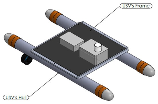
Figure 2.
USV CAD design.
The materials chosen to manufacture the USV are easily found on e-commerce or the market. The manufacturing of the USV is undertaken by a simple machining process (grinding, sawing, and boring) and a simple joining process (fastening).
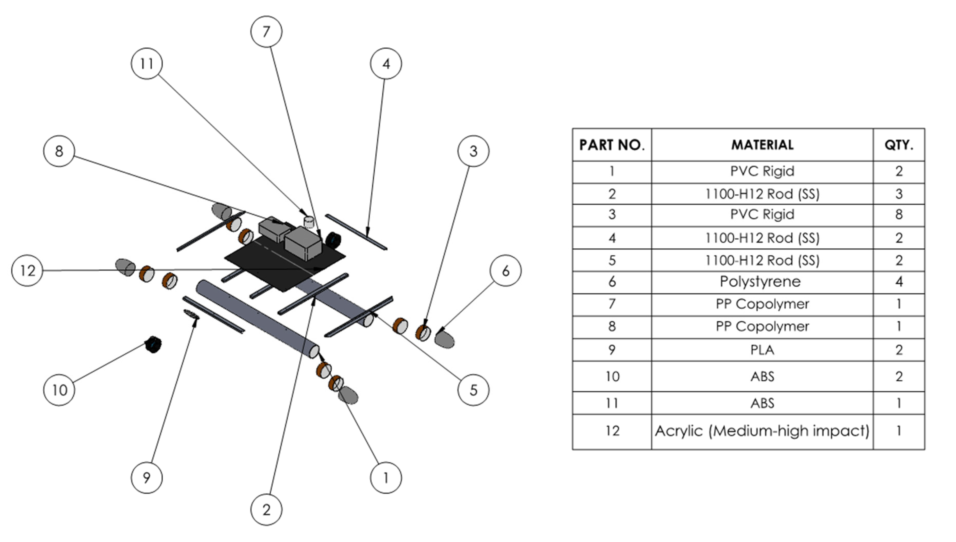
The selected materials of the USV design are presented in Figure 3. Sturdy and lightweight materials are used for the Frame. Lightweight, sturdy materials with high buoyancy are appropriate to be applied for the hull whilst non-corrosive materials and lightweight material are obligatory for the thruster.
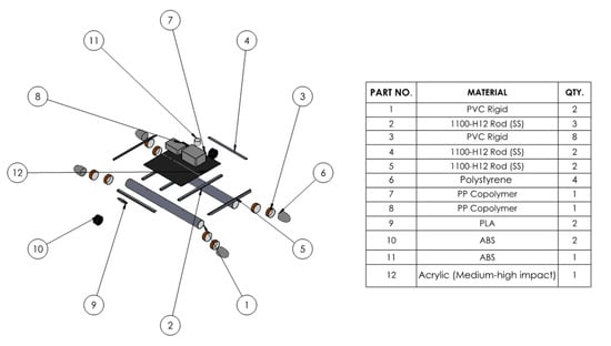
Figure 3.
Exploded view dan materials of the proposed USV.
According to the design analysis obtained in SolidWorks, the mass of designed USV is 4217 g. The USV is equipped with a battery (440.5 g); Pixhawk controller (33.1 g); other components, such as compass, GPS, Telemetry, Buzzer (25 g), Go Pro action camera; and its holder (250 g). Therefore, the total mass of the USV is 4965.6 g, 4.97 in kg, or 48.76 N, while the total volume of which is 5316 cm3, or 0.005316 m3.
3.2. Electrical Wiring
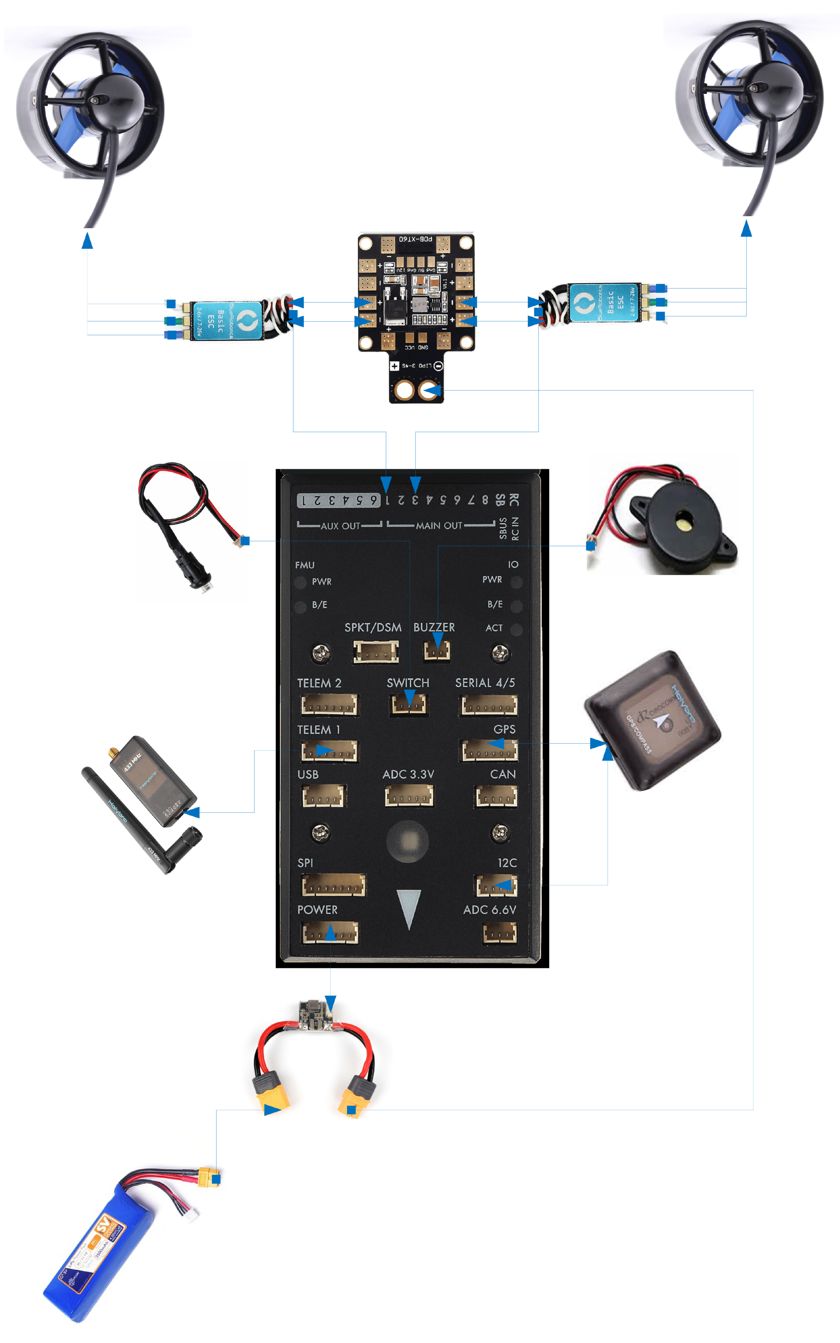
The wiring diagram for the mechatronics components is shown in Figure 4. Holybro PIX32 Pixhawk controller was selected to regulate commands for heading and steering. The controller is integrated with the necessary sensors to operate for example 3-axis gyroscope and a 3-axis accelerometer. The package includes a 168 MHz CPU with 256 KB of RAM. The electronics speed controller (ESC) from Blue Robotics controls the speed of the motor on the thruster to generate thrust for driving the USV motion. The ESC has a maximum current of 30 A and an operating voltage of 7–26 Volts (2–6 s). T-100 thruster is preferred as a propulsive device used for attitude control. The thruster can generate a maximum thrust of around 5.2 lbf. Hyperion Lithium polymer battery is utilized as the power supply for the USV system. The selected battery is 2500 mAh, three cells (3 s), with a nominal voltage of 3.7 V per cell. Holybro Telemetry Radio 915 MHz is chosen as the wireless data communication between the USV and ground control station (GCS). The maximum wireless communication range is around 1.6 km. Remote control (RC) transmitter-receiver is used for remote command from a pilot. Holybro Buzzer is employed as an indicator for the completed process, or an error occurs in a controller. Holybro Power Modul is applied to distribute energy supply from the battery to the controller. Holybro Micro M8N Compass and GPS are sensors implemented as navigation device for the USV. Even though IMU and GPS are sensitive to the magnetic environment, they are lightweight and small in size, and have low energy consumption, which are important advantages for USV [4].

Figure 4.
Wiring diagram for the USV controller.
Additionally, apart from its compatibility with open-source ground control stations, the essential aspect of choosing Holybro products is its price. All Holybro items shortlisted above only cost $180. As a result, the total cost is roughly $524.97 in which $246.46 is allocated for the T-100 Blue Robotics thruster, $27.95 for the battery, and about $70.42 for frame material and manufacturing process. Whilst the Notebook Computer and the remote control are an asset which has been ready. Compared with an affordable Unmanned Surface Vehicle developed by Zhou et al., this cost is steeply low as its price is highly under $3000 [11]. The development cost is the same as the USV developed by Mancini A. et al. which lower than €1000 or $1131.07 [23].
4. Design Analysis
In prototyping the USV, it is vital to comprehensively analyze several aspects to ensure that USV works properly and is safe, which are outlined in the following.
4.1. Buoyancy
One essential aspect analyzed in the USV design process is the buoyant force generated by the USV. The buoyant force needs to be calculated to determine whether the buoyant force of USV can lead the USV to float. The criteria, which have to be met is the buoyant force of the USV, is greater than the weight of the USV (Fb > W). The buoyant force equations are presented in Equations (22)–(24). Where Fb is buoyant force (N), is water density (kg/m3), g is the acceleration of gravity (m/s2), and , different from the total volume of USV (0.005316 m3), is the sum of USV’s Frame, Thrusters, and Hulls volume (m3) or the volume of the submerged part.
From the results of this calculation, where W = 48.76 N, the value of Fb > W was found. It is concluded that the USV is floating. However, due to the fact that the value of buoyant force (Fb) is approximately the USV’s weight, almost all of the hull and the Frame are submerged.
4.2. Required Thruster
To calculate the required thruster power, it is assumed that USV only moves straight or longitudinally. The USV Equation of Motion (EOM) when moving in the longitudinal direction is served in Equation (8). By neglecting the lateral speed, and yaw rotation, the EOM is expressed in Equation (25).
To calculate the minimum required thrust, Equation (25) is calculated during stationary conditions. As a result, Equation (25) is derived as
where is the total linear drag force in u direction calculated using Equation (28).
where is defined as linear drag force that works around the Frame of USV in u direction, while is linear drag force around each hull of the USV in the u direction. These are calculated by Equations (29) and (30).
where is the drag coefficient of USV Hull, is the density of water, g is the gravity acceleration, u is the longitudinal velocity of USV, is the frontal area of USV’s Hull, is the frontal area of USV’s Frame. In this work, the desired longitudinal velocity is 1.3 m/s, = 997 kg/m3, g = 9.81 m/s2, , , [24], [24].
The calculation results show that and . Consequently, the sum of linear drag force () and the total thrust force of USV that is required when sailing in 1.3 m/s is 28.02 N or should be around 6.29 lbf. According to this result, the T-100 thruster from Blue Robotics meets this criterion since the maximum thrust of a single thruster is 5.2 lbf.
4.3. Stability Analysis
Stability analysis is conducted by roll stability study. The result of the roll stability test is presented in Figure 5.
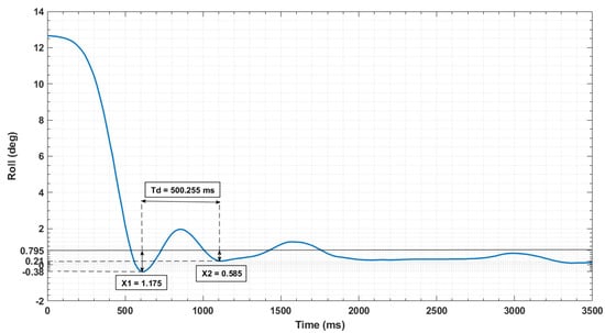
Figure 5.
Roll stability test result.
From the obtained result in Figure 5 at the initial condition, a 5 kg load is put on the right side of the USV. The USV will be tilted to the right by 12.66° then it will be tilted to the left by 0.36°. Afterward, on the second roll, the USV is tilted to the left by 1.97° and next tilted to the right 0.21° until it reaches a stable position or at around 0°. The roll reduction between the first roll and the second roll is 86.5%.
In terms of the graph analysis using the logarithmic decrement method is acquired, with the value of damped period (Td) around 0.5 s, damped natural frequency (ωd) is 12.56 rad/s, and natural frequency (ωn) is 12.63 rad/s. The calculated damping ratio is 0.11. To conclude, this USV is moderately stable even though the damping ratio is quite small.
5. Design Implementation
The manufacturing process begins with cutting aluminum parts by grinding process to fit the specific dimensions in the design documentation, and then holes are produced in aluminum parts through the boring process. The assembly, carried out between the aluminum plates and the hull, was conducted by the fastening process. After the assembly process has been completed, the thruster installation is performed on the left and right hulls. Before installing the thruster, the bracket is installed first.
An acrylic is placed in the Frame of the USV. Two containers are installed to place Pixhawk controller, batteries, and sensors. The battery containers are placed behind the container that contains the controller and sensors. At the top of the container, the GPS/compass module is installed. This location is selected to prevent magnetic interference caused by other electrical components. Telemetry is installed beside the container so that the transmitted and received signals are not problematic. Additionally, the camera is assembled at the top of the container for documentation purposes. The joining method is a fastening method using bolts and nuts. In this phase, aluminum foil coating is also applied on the battery container to reduce the heat transfer from solar radiation.
Finally, the nose is manufactured and installed. The nose comprises styrofoam material and is shaped through the sanding process after the nose is taped to the dop. The manufacturing result of the proposed USV is depicted in Figure 6.
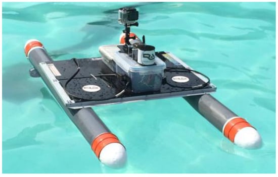
Figure 6.
The result prototype of USV.
6. Guidance Navigation and Control (GNC)
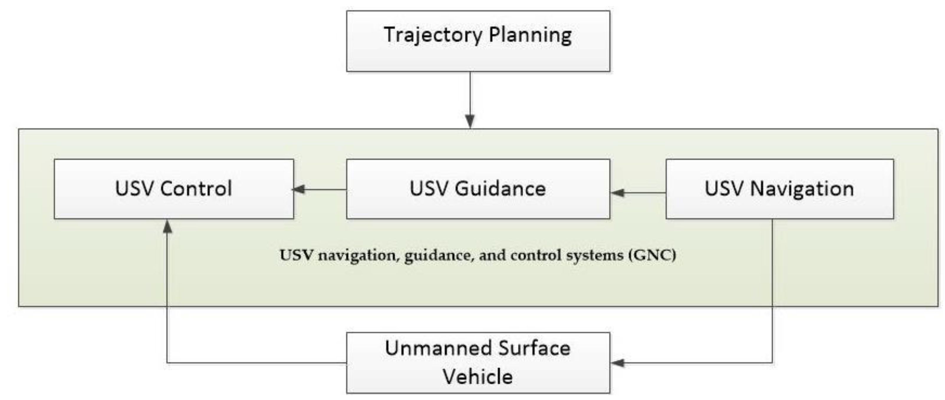
In unmanned vehicle navigation, Guidance and Control Systems (GNC) is responsible for obtaining the vehicle’s current location relative to a reference coordinate to determine the path and speed of USV [25]. and calculates the necessary forces that each one of the actuators must produce. The interaction of GNC with USV/vehicle is shown in Figure 7.
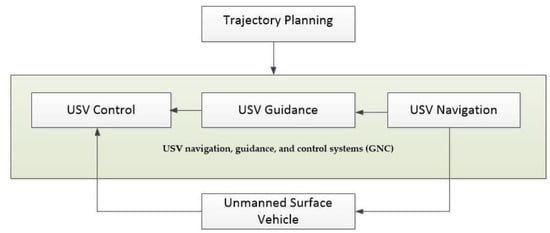
Figure 7.
Interaction among GNC and vehicle.
6.1. Guidance
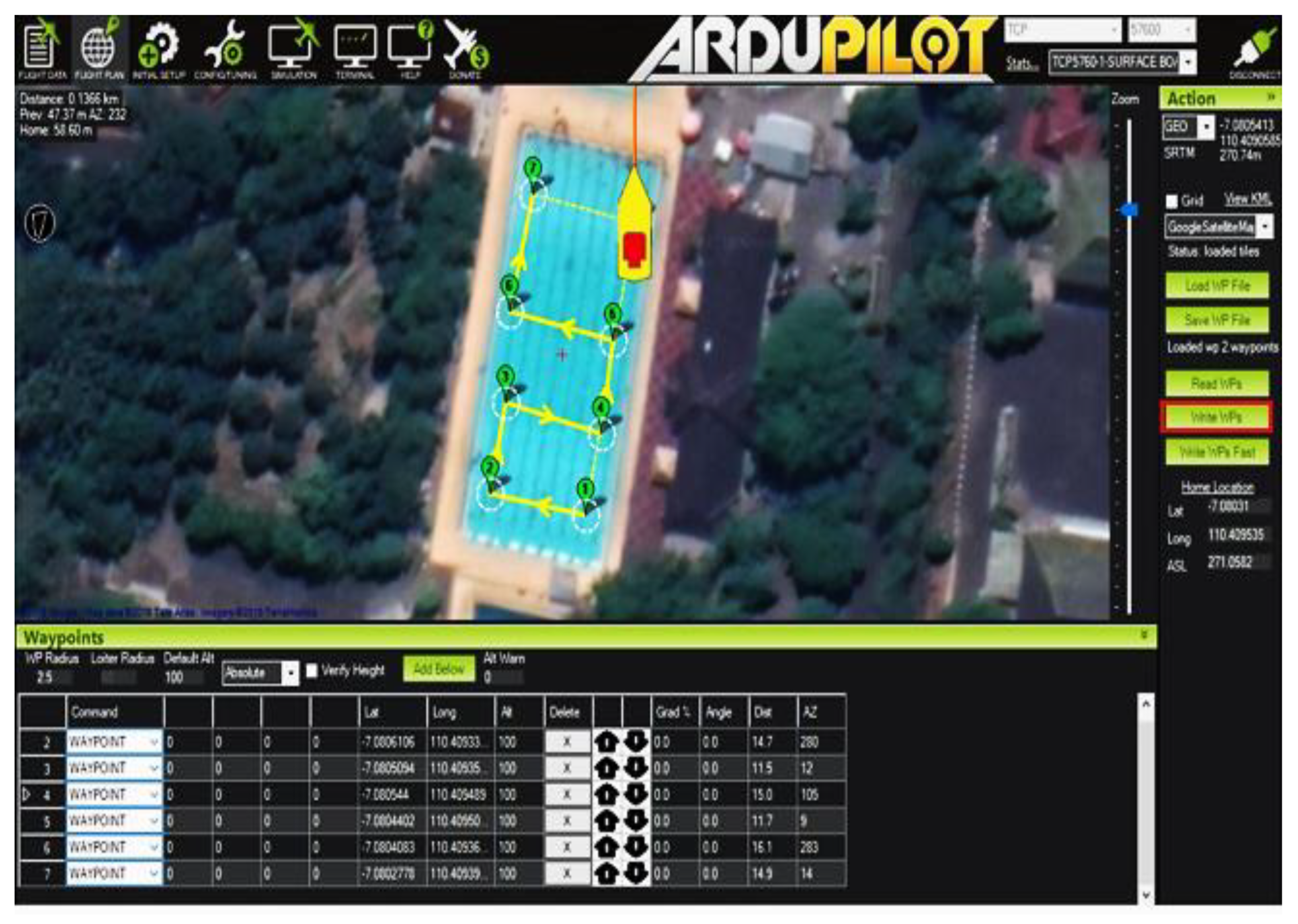
Guidance is usually executed based on data from the Global Navigation Satellite System (GNSS) and motion sensors such as accelerometers or gyroscopes. In the guidance system, the sailing path of USV is determined by path planning. Path planning refers to the system responsible for designing paths for autonomous missions [26]. The path planning process includes two main steps: the determination of a set of points on the map (waypoint), shown in Table 2, and the generation of a path based on the waypoints Figure 8. Zigzag trajectory has been selected as it is commonly used in bathymetry missions.
Table 2.
Waypoint data.

Figure 8.
Path generation.
In addition, the cruise speed and cruise throttle parameter values are determined in the guidance system. When USV sailing follows the path, the cruise speed is the target speed in meters per second, while the cruise throttle is an estimate of how much throttle is needed in percent to attain cruise speed when sailing straight ahead. In this case, cruise speed value is given at 1.3 m/s.
6.2. Navigation
The navigation parameter settings in this study were determined using the Mission Planner software. There are two essential parameters that need tuning. Turn G max, for example, indicates the maximum lateral acceleration (in multiples of 9.81 m/s2) that a USV can withstand while staying stable. The USV may tip over in turns if it is set too high, and the USV will not be able to turn sharply enough if it is set too low. The Lateral Acceleration Period (Lat Acc Control Period) is the parameter for aggressiveness control. Raising the LatAcc Cntrl Period if the USV weaves along the straights, lowering it if the USV does not turn sharply enough.
For this research, the turn G maximum lateral acceleration is given 5 m/s2, and the lateral acceleration central period is given 20 s. These parameters depend on the shape of USV and are obtained experimentally.
6.3. Control
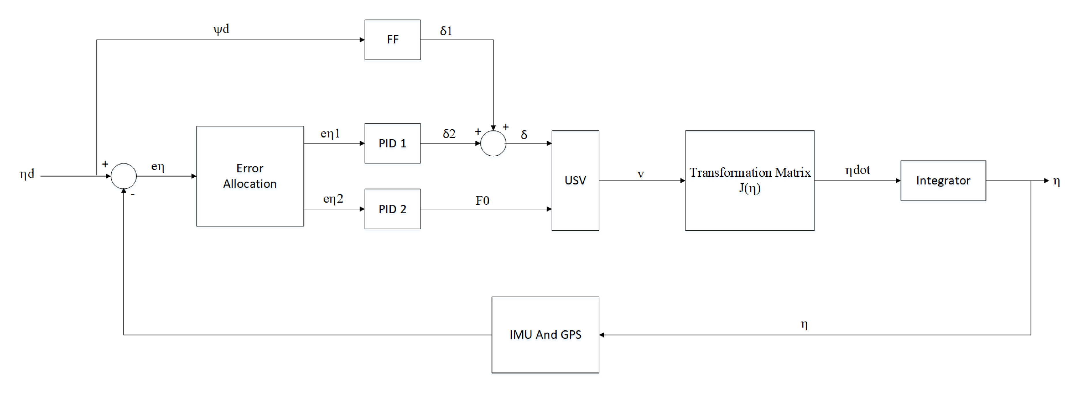
Control is the action of determining the necessary forces and moments produced by thrusters so that USV moves following the path. Proportional Integral Differential (PID) control is employed to control USV speed, and that integrated with Feed Forward (FF) control is implemented to control steering rate. Feed Forward control is included for enhancing response performance (to minimize the error between the current state of the system and the desired state). This combination is commonly benefited for autonomous mission purposes due to its significant contribution to eliminating disturbance and enhancing the controller’s performance for an autonomous system [27,28]. The control block diagram of the USV is shown on the block diagram in Figure 9.
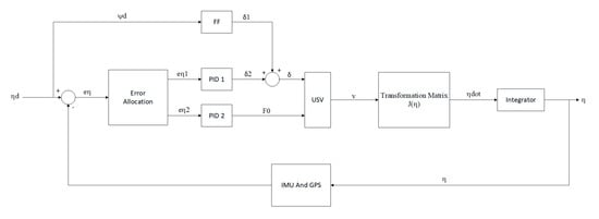
Figure 9.
Control scheme employed on the proposed USV.
The motion of USV is controlled by PID compensator, where the output of the PID controller is in the form F0 and δ. The applicable equation to determine the F0 and δ values are written in Equations (31) and (32). Where is the longitudinal error position of USV, and is the Heading Error of USV.
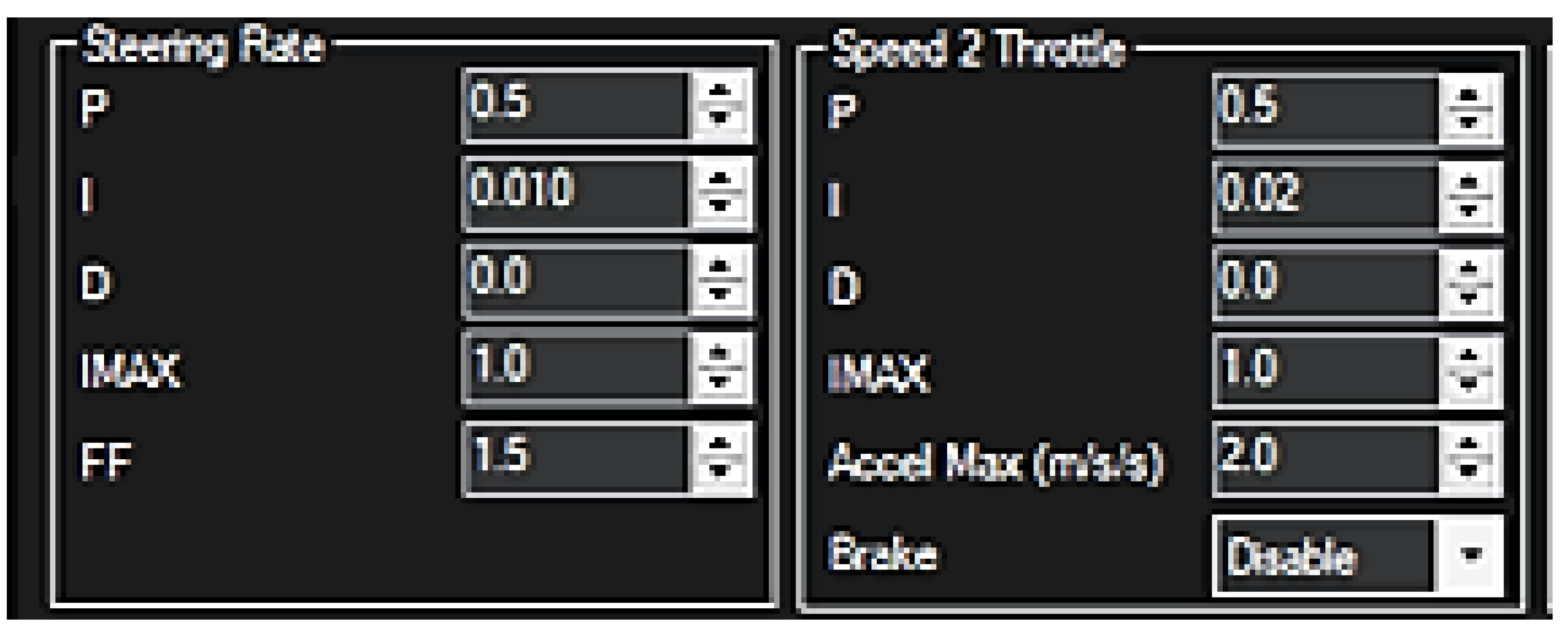
In this work, the PID Gains were obtained experimentally to control the Throttle (KP2, KI2, KD2), which is 0.5 for the p-value and 0.01 for the value of I. While the PID and FF Gain obtained to control Steering Rate (KP2, KI2, KD2, KFF) is 1.5 for the FF value, 0.5 for the p-value, and 0.01 for the value of I, as shown in Figure 10.
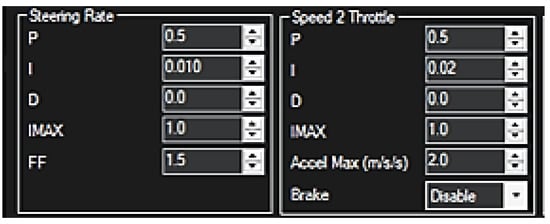
Figure 10.
PID control tuning parameter.
The GNC process is managed and monitored by the Ground Control Station (GCS). Moreover, it is software operated to monitor USV status when in operation under FPV (First-person View). The GCS Software selected and adopted in this study is Mission Planner. The full-featured GCS can be used as a GCS from various platforms, for instance, an aircraft, helicopter, drone, rover, and boat. Michael Oborne developed this software, and it is open-source. This software is only compatible with Windows. With Mission Planner, sailing data mined from GPS, IMU, and other sensors are exposed in the screen of GCS. For example, Figure 11 presents the information data from the IMU sensor, such as heading, ground speed, and position data from GPS, battery level, and communication signal strength. Moreover, as a GCS, Mission Planner is also able to set up, config., and tune a USV for optimum performance.
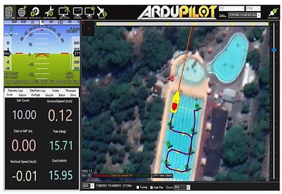
Figure 11.
Ground Control Station (GCS).
7. Experimental Results
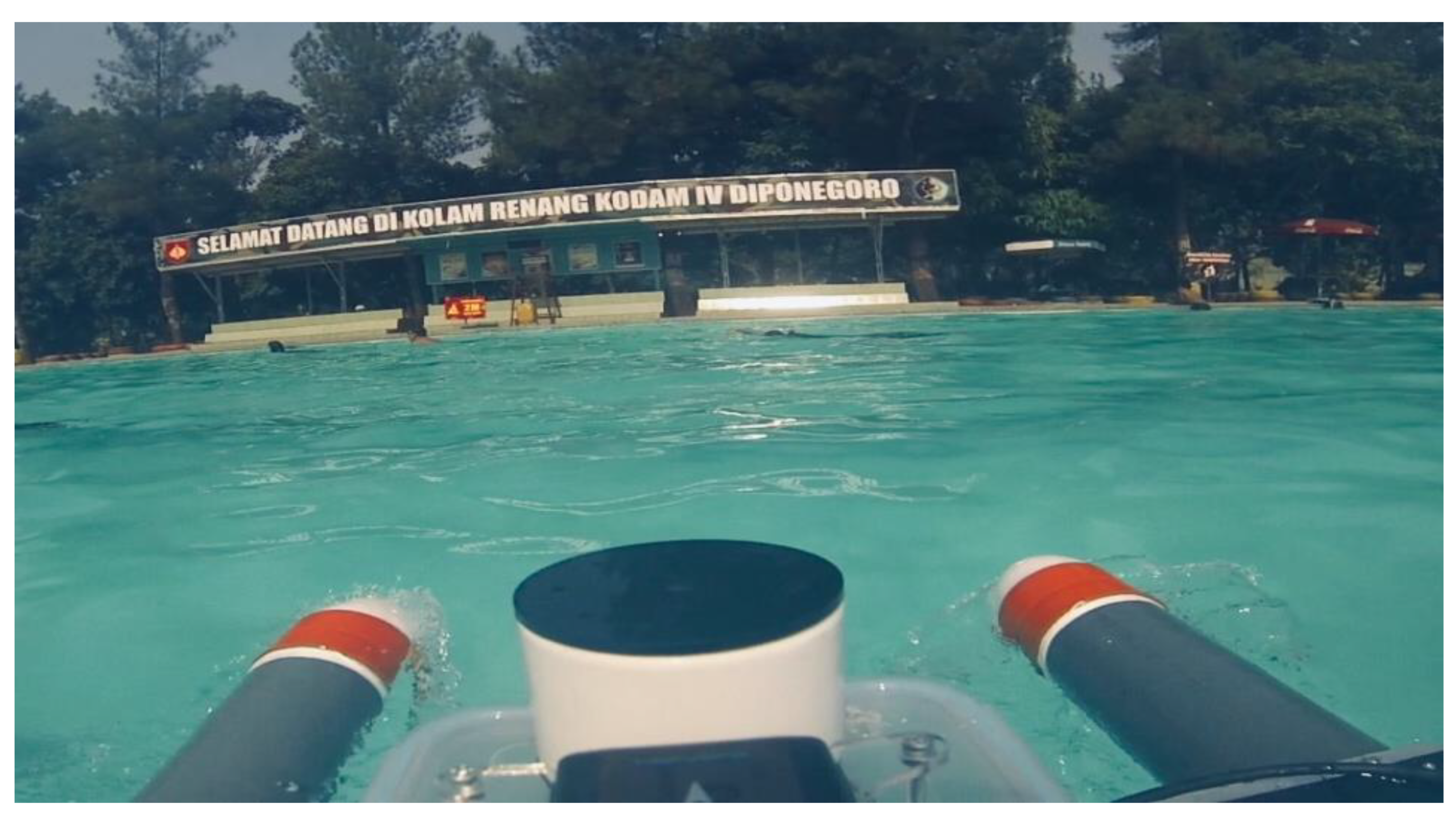
The research was performed at a swimming pool located at the military camp area in Semarang, Indonesia (Figure 12) when the disturbance of sea currents or wind waves can be neglected. In this work, the results of compass accuracy measurement are based on magnetic field data, and GPS accuracy measurement is according to satellite and (Horizontal Dilution of Precision) HDOP data. The USV performance measurement is based on trajectory and energy consumption data.

Figure 12.
Military camp’s swimming pool.
7.1. Compass Accuracy Measurement
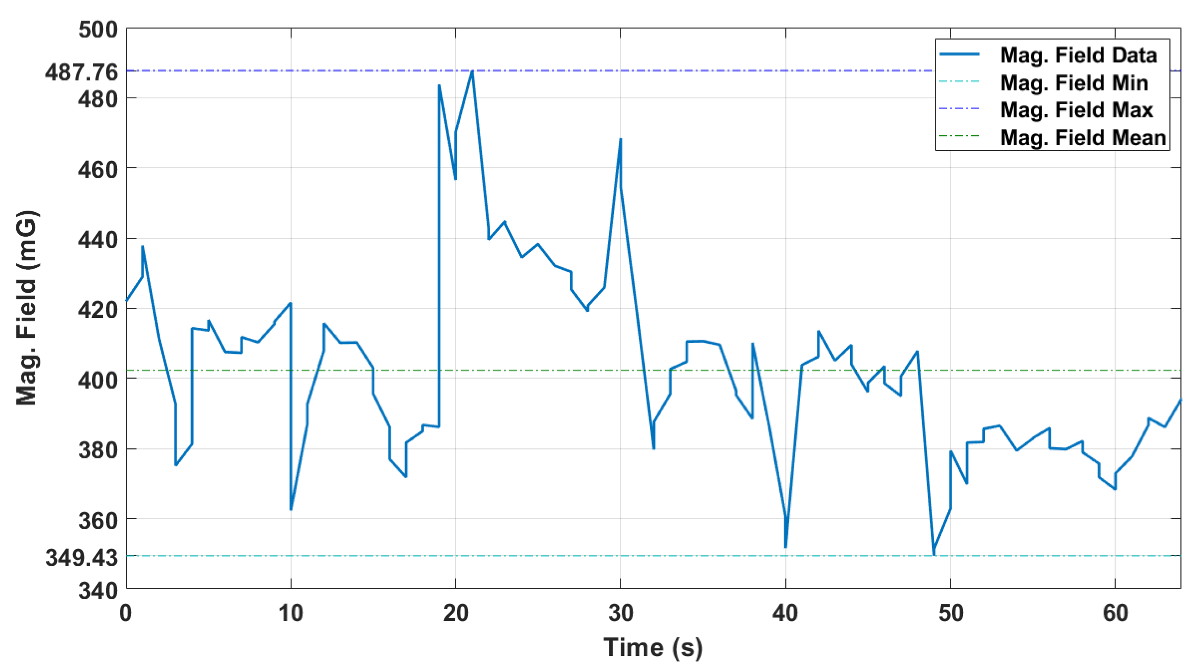
Compass accuracy depends on the calibration before the USV sailing. If the calibration procedure is carried out correctly, direction disorientation cannot occur. The compass accuracy also depends on magnetic interference around the compass. This relates to the position of compass placement if the compass is placed on hardware with strong magnetic properties or devices with large electromagnetic radiation. Compass accuracy will be reduced if the interference is very large, it can cause disorientation heading of the USV. To determine the magnitude of interference in the compass is done by analyzing the graph that shows the magnitude of the Magnetic Field versus time; the interference is large if the deviation of the maximum Magnetic Field value from the average value on the graph is above 60%. In addition, the interference is negligible if the deviations occur below 30%. While for the range between 30% to 60%, the amount of interference is moderate [29]. Magnetic field data obtained when the USV is sailing with the autonomous mode are presented in Figure 13.
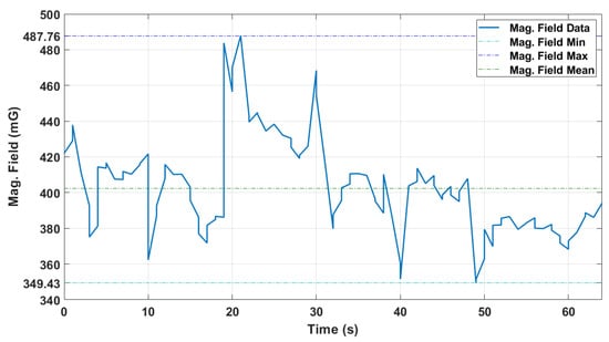
Figure 13.
Magnetic field versus time.
According to Figure 13, it can be interpreted that the greatest magnetic field deviation from the mean is 487.76 mG, or around 21.23% of the mean. From the analysis results, it is concluded that the amount of interference that occurs in the compass is small due to magnetic field deviations, which are still below 30%. Additionally, from the study, the data rate of the compass is about 1.68 bytes/s.
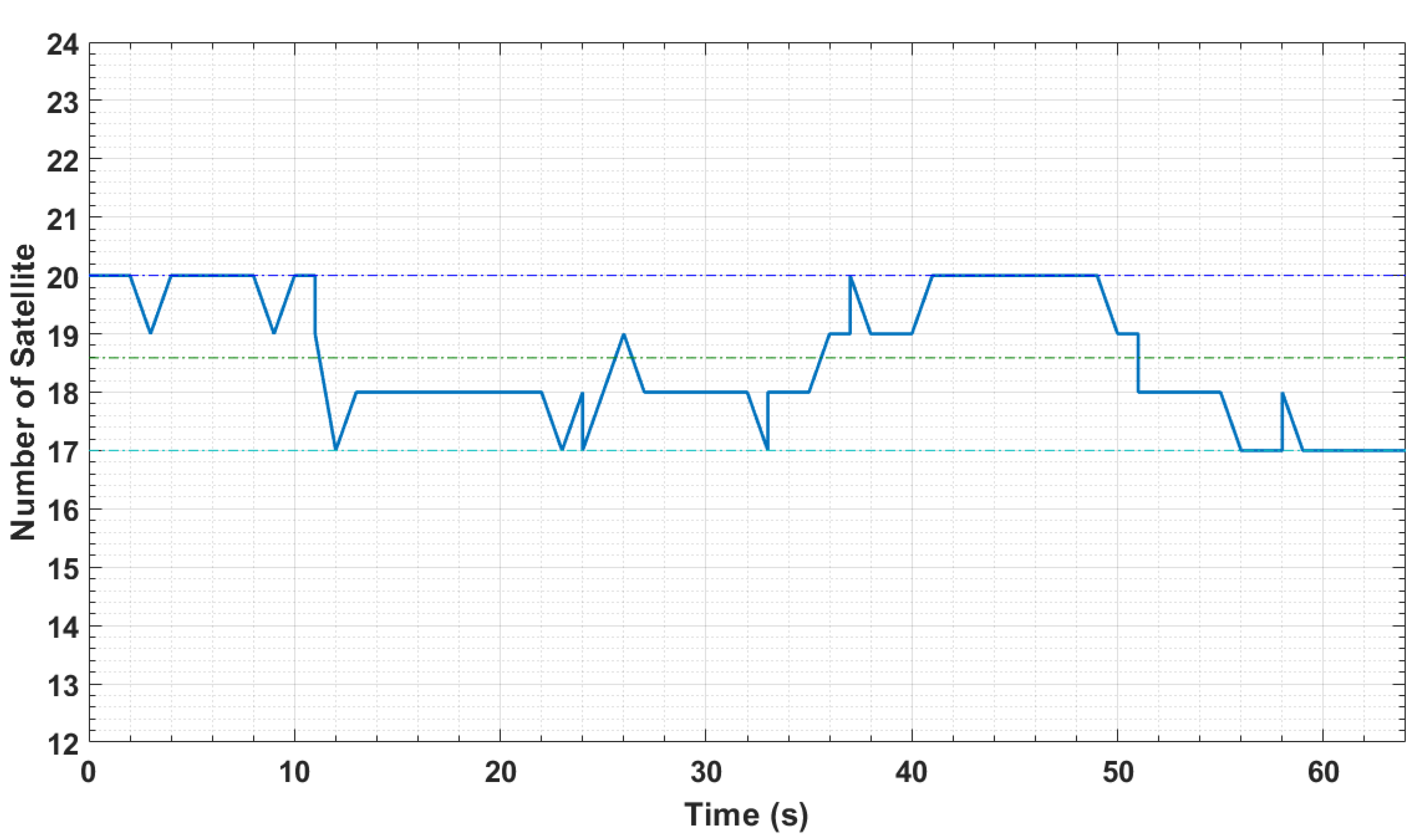
7.2. GPS Accuracy Measurement
Similar to compass, GPS accuracy depends on the calibration before the USV moves. If the calibration procedure is performed correctly, a disorientation position could not occur. Besides, GPS accuracy is also determined by the number of satellites that GPS reads. The minimum number of satellites is 12 satellites from 32 satellites [29]. The more satellites are read, the more accurate the position is read by GPS. The number of satellites when sailing with the Autonomous mode in this work can be seen in Figure 14. The conclusion drawn from the graph in Figure 14 is the minimum number of satellites that GPS reads as many as 17 Satellites. Meanwhile, the GPS data rate acquired is around 1.52 bytes/second.
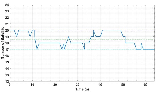
Figure 14.
The number of satellites read by GPS on the USV.
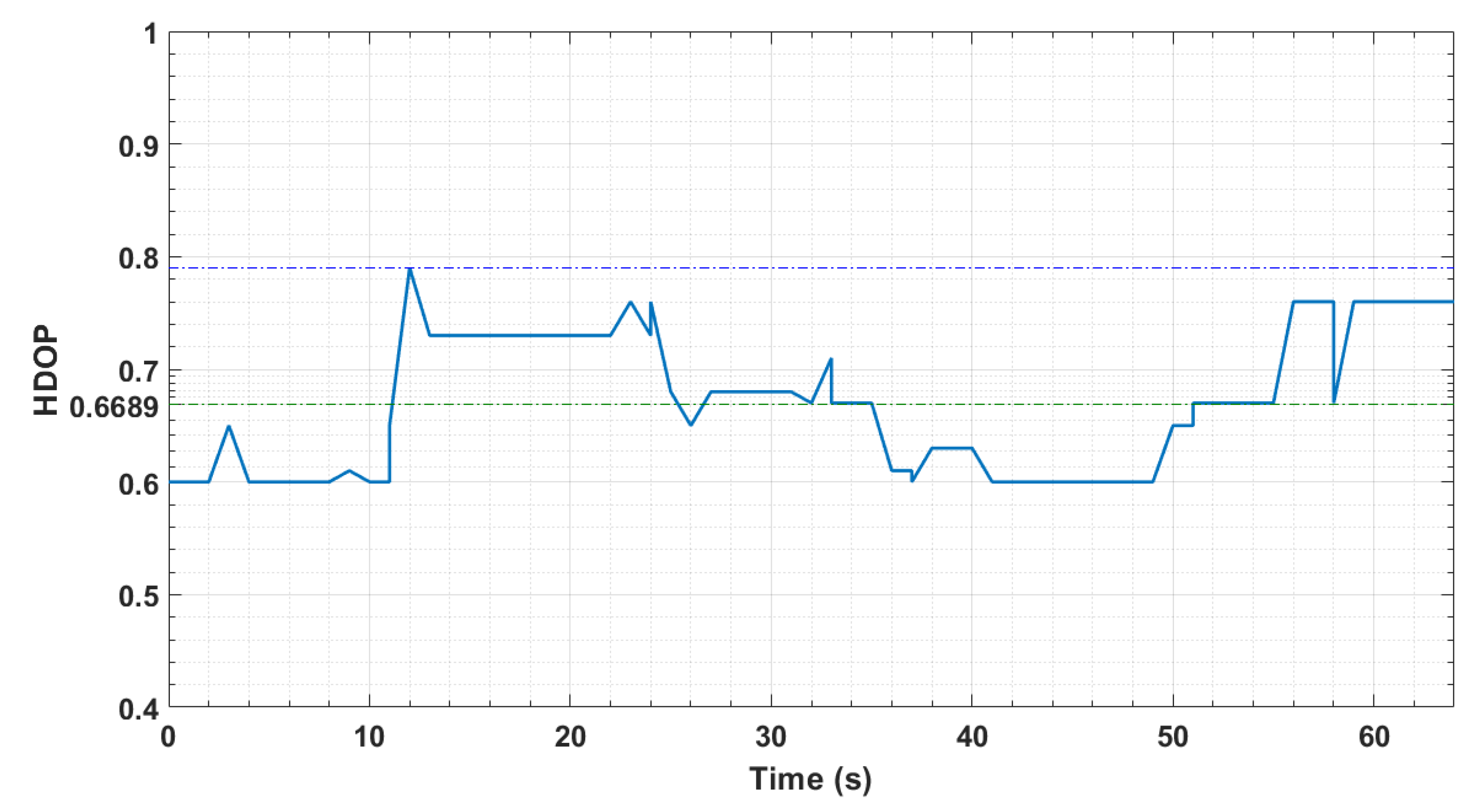
Another technique for analyzing GPS accuracy is to analyze the Horizontal Dilution of Precision (HDOP) value of GPS, a number used to express the horizontal geometric strength of the satellite constellation. GPS accuracy is significant if the HDOP value is below 1.5 and is very poor if above 2 [29]. Graph HDOP versus time when USV sailing is plotted in Figure 15. The conclusion drawn from the graph is the maximum HDOP value is 0.8, and the HDOP value vacillates between 0.6 and 0.8, which according to other studies, indicates high signal quality [17]. The final conclusion is that the accuracy value of a GPS is large because the HDOP value is below 1.5 and the number of satellites read by GPS is above 12 satellites.
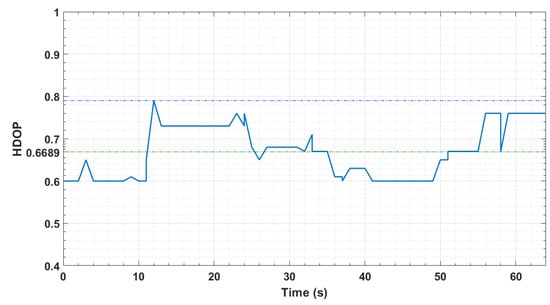
Figure 15.
HDOP values versus time variables.
7.3. Trajectory Measurement
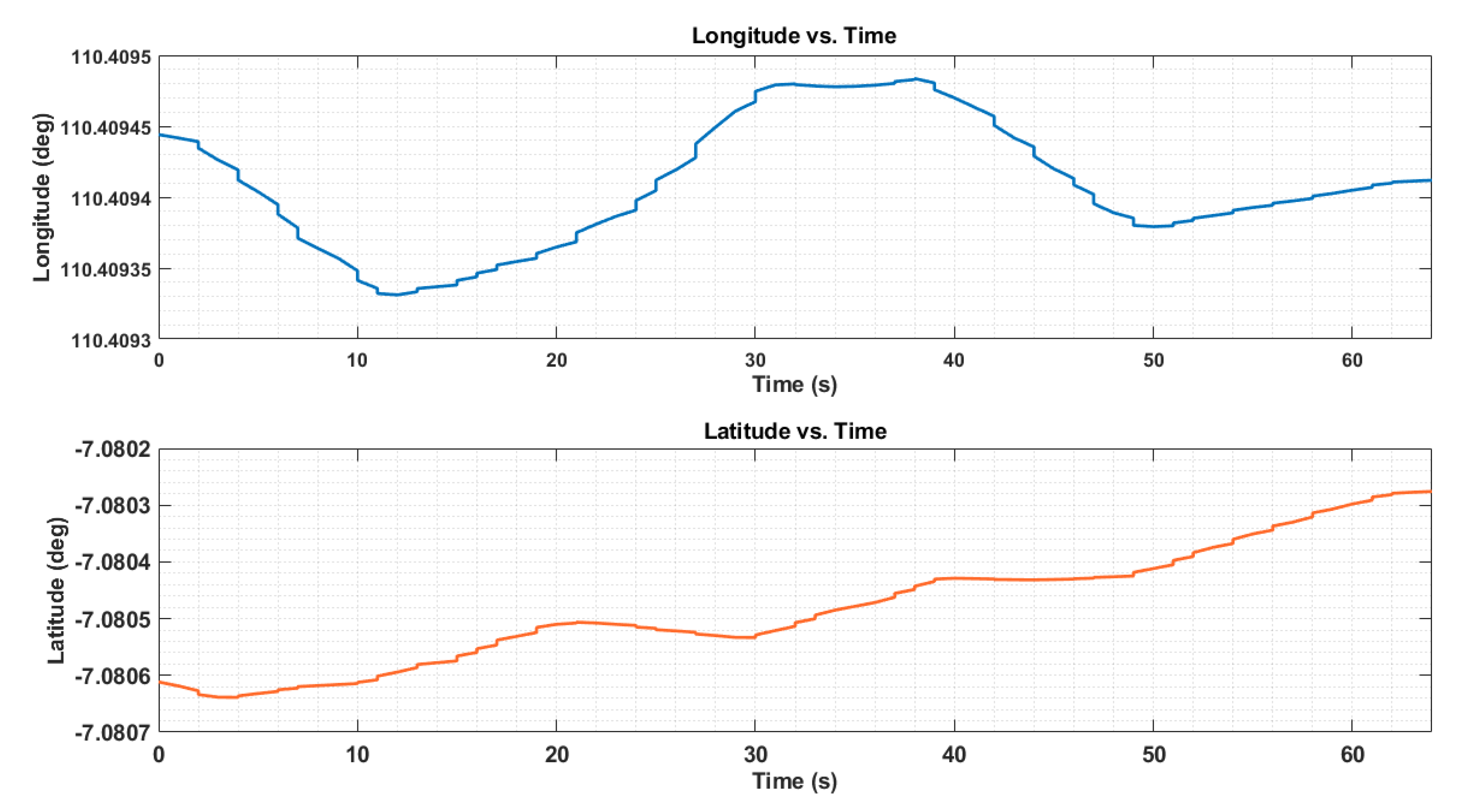
The data position of USV is defined in the form of longitude (latitude) and latitude (longitude). The plot of longitude and latitude versus time is depicted in Figure 16. Longitude indicates the position in the west or east of the Prime Meridian line while latitude is the position in the south or north of the Equator [30]. The unit of longitude and latitude in this research is the Decimal Degree (DD). Figure 16 depicts a plot of measured longitude and latitude vs. time. The position data is obtained at a rate of 1.33 bytes/second when the USV is sailing along at 31.62 m within 64 s. The longitude and latitude were acquired using GPS. The measured data were sent from the USV to the GCS on the computer using wireless transceiver. While the latitude and longitude commands were generated and sent from GCS on PC to the USV.
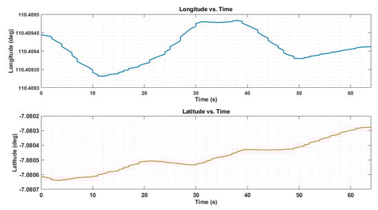
Figure 16.
Measured longitude and latitude.
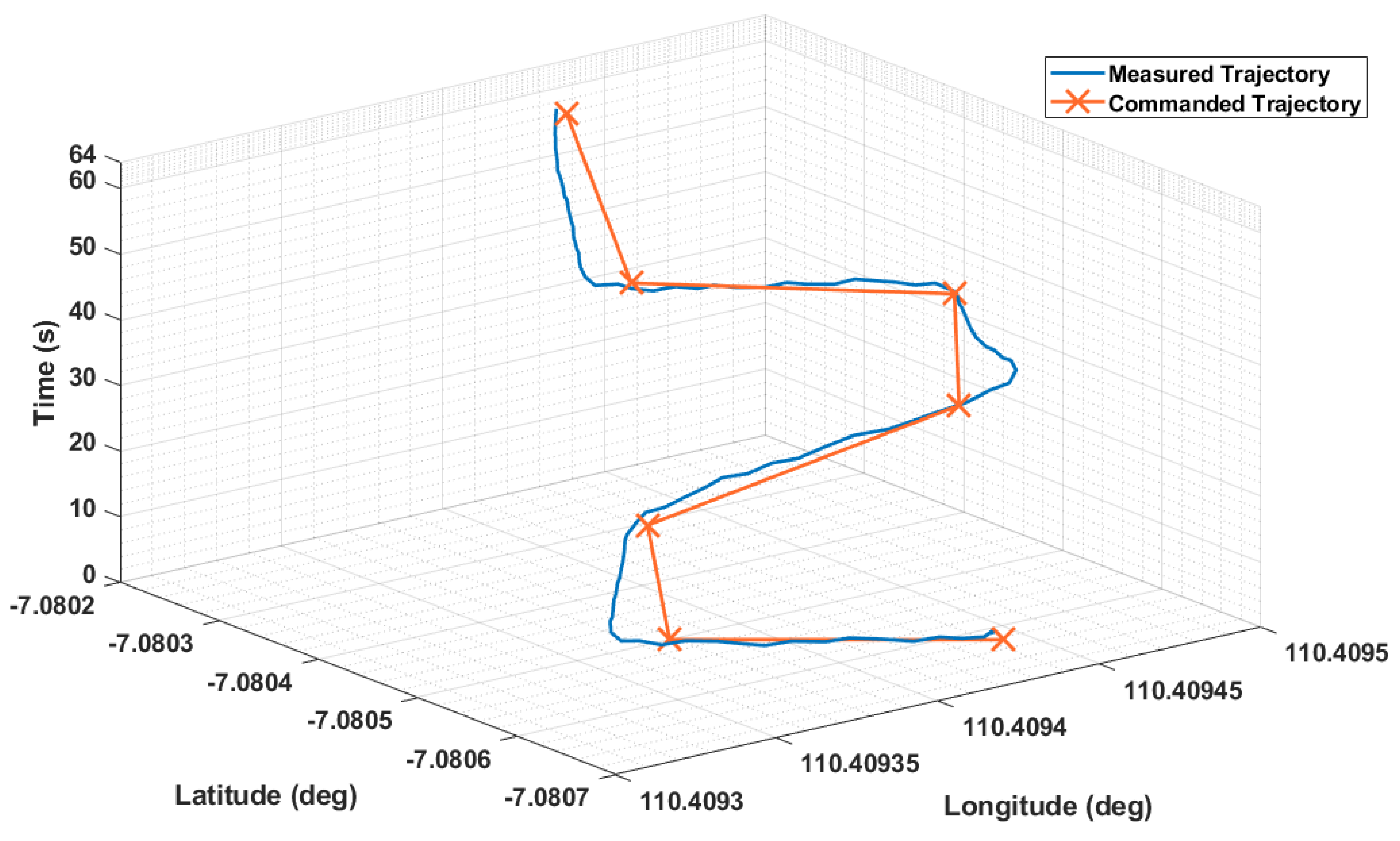
The comparison of positions between the commanded and measured trajectory of USV towards the time is depicted in Figure 17. The error calculation found that the Root Mean Square Error (RMSE) was about 0.99 m, and the average of Cross Track Error (CTE) was around 0.86 m. The RMSE is not considerably different from that of the USV developed by Chunyue et al. in which experimental testing for a zigzag path revealed it to be 0.54 m [19]. While from the prior study by Marchel, USV equipped High-Precision RTK Receiver and speed of 2.5 km or 1.3 m/s were acquired at 0.919 m for the average of CTE. It concludes that The effect of RTK Receiver for zigzag path-following is not considerably high compared to the performance of USV; this is in line with the conclusion that has been revealed [17].
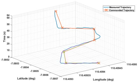
Figure 17.
Commanded versus measured USV trajectory.
7.4. Energy Consumption Measurement
To determine the battery performance of USV, energy consumption is calculated. The measurement of energy consumption is retrieved every second when the USV sail is in autonomous mode, as plotted in Figure 18. The figure shows that to complete an autonomous mission in 64 s with a predetermined path, the energy consumption is 5900 J. From this data, it is concluded that the USV is able to sail for 6.02 min with 0.18 km cruising capability.
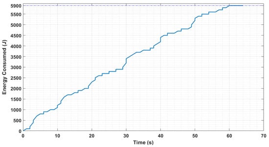
Figure 18.
Energy consumption for 70 s.
8. Conclusions
In this work, Proportional integral Differential (PID) and Feed Forward (FF) control for a proto-type Unmanned Surface Vehicle (USV) have been executed. This type of controller is suitable for use for a USV autonomous mission; however, it can be seen from experimental data that it works well for the straight line, but the error is moderately high for turning; thus, more experimental testing for determining FF gain is essentially needed.
This paper also proved that adding an RTK does not substantially influence the performance of USV, but future study is necessary to explore a non-zigzag trajectory. Moreover, to develop a USV for data retrieval missions in calm seas and shallow waters, the simple combination of PID controller and open-source GCS software is adequate; therefore, the high cost and complexity of the algorithm for USV development is not necessary. Further research is needed for Aerodynamics analysis to define which model is suitable for certain applications and areas, and which is effective to reduce energy consumption. The greater hull dimension is necessary for the Frame not to be submerged; hence the probability of the electrical component being waterlogged can be reduced.
Author Contributions
Conceptualization, J.D.S. and M.A.S.; methodology, M.A.S.; software, M.A.S.; validation, J.D.S., M.A. and W.C.; formal analysis, M.A.S. and M.A.; resources, S.A.; data curation, M.A.S.; writing—original draft preparation, J.D.S., M.A.S. and M.A.; writing—review and editing, M.A.S., M.A., W.C. and M.S.; visualization, M.A.S.; supervision, J.D.S., W.C. and M.M.; project administration, S.A.; funding acquisition, W.C. and M.S. All authors have read and agreed to the published version of the manuscript.
Funding
This research received no external funding.
Conflicts of Interest
The authors declare no conflict of interest.
References
- Putri, F.T.; Ariyanto, M.; Haryanto, I.; Arozi, M.; Caesarendra, W.; Hanan, M.R.I. Development of Unmanned Aerial Vehicle (UAV) ornithopter with wireless radio control. In Proceedings of the 2016 3rd International Conference on Information Technology, Computer, and Electrical Engineering (ICITACEE), Semarang, Indonesia, 19–21 October 2017; pp. 79–84. [Google Scholar]
- Harfina, D.M.; Zaini, Z.; Wulung, W.J. Disinfectant spraying system with quadcopter type unmanned aerial vehicle technology as an effort to break the chain of the covid-19 virus. J. Robot. Control 2021, 2, 502–507. [Google Scholar]
- Alshorman, A.M.; Alshorman, O.; Irfan, M.; Glowacz, A.; Muhammad, F.; Caesarendra, W. Fuzzy-based fault-tolerant control for omnidirectional mobile robot. Machines 2020, 8, 55. [Google Scholar] [CrossRef]
- Balestrieri, E.; Daponte, P.; De Vito, L.; Lamonaca, F. Sensors and measurements for unmanned systems: An overview. Sensors 2021, 21, 1518. [Google Scholar] [CrossRef] [PubMed]
- Ball, M. USV Performs Offshore Data Harvesting in North Sea 2019. Available online: https://www.unmannedsystemstechnology.com/2019/09/usv-performs-offshore-data-harvesting-in-north-sea/ (accessed on 19 January 2020).
- Stenersen, H.S. Construction and Control of an Autonomous Sail Boat; Norwegian University of Science and Technology: Trondheim, Norway, 2015. [Google Scholar]
- Setiawan, J.D.; Chrismianto, D.; Ariyanto, M.; Sportyawan, C.W.; Widyantara, R.D.; Alimi, S. Development of Dynamic Model of Autonomous Sailboat for Simulation and Control. In Proceedings of the 2020 7th International Conference on Information Technology, Computer, and Electrical Engineering (ICITACEE), Dubai, United Arab Emirates, 18–19 December 2020; pp. 52–57. [Google Scholar]
- Setiawan, J.D.; Arief Budiman, B.; Ariyanto, M.; Andromeda, T.; Chrismianto, D.; Aziz, M.A. Experimental Study on the Aerodynamic Performance of Autonomous Boat with Wind Propulsion and Solar Power. In Proceedings of the 2019 6th International Conference on Electric Vehicular Technology (ICEVT), Ungasan, Bali, 18–21 November 2019; pp. 213–219. [Google Scholar]
- Barrera, C.; Padron, I.; Luis, F.S.; Llinas, O.; Marichal, G.N. Trends and challenges in unmanned surface vehicles (Usv): From survey to shipping. TransNav 2021, 15, 135–142. [Google Scholar] [CrossRef]
- Manley, J.E. Unmanned Surface Vehicles, 15 Years of Development. In Proceedings of the OCEANS 2008, Quebec City, QC, Canada, 15–18 September 2008; pp. 1–4. [Google Scholar]
- Zhou, M.; Shi, J. The Design and Development of an Affordable Unmanned Surface Vehicle for Estuary Research and STEM Education. In Proceedings of the Global Oceans 2020: Singapore–US Gulf Coast, Biloxi, MS, USA, 5–30 October 2020. [Google Scholar]
- Bae, J.H.; Min, B.C.; Luo, S.; Kannan, S.S.; Singh, Y.; Lee, B.; Voyles, R.M.; Postigo-Malaga, M.; Zenteno, E.G.; Aguilar, L.P. Development of an unmanned surface vehicle for remote sediment sampling with a van veen grab sampler. In Proceedings of the OCEANS 2019 MTS/IEEE SEATTLE, Seattle, WA, USA, 27–31 October 2019. [Google Scholar]
- Iovino, S.; Savvaris, A.; Tsourdos, A. Experimental Testing of a Path Manager for Unmanned Surface Vehicles in Survey Missions. IFAC-PapersOnLine 2018, 51, 226–231. [Google Scholar] [CrossRef]
- Mou, J.; He, Y.; Zhang, B.; Li, S.; Xiong, Y. Path following of a water-jetted USV based on maneuverability tests. J. Mar. Sci. Eng. 2020, 8, 354. [Google Scholar] [CrossRef]
- Sutton, R.; Sharma, S.; Xao, T. Adaptive navigation systems for an unmanned surface vehicle. J. Mar. Eng. Technol. 2011, 10, 3–20. [Google Scholar] [CrossRef] [Green Version]
- Huayna-Aguilar, M.M.; Cutipa-Luque, J.C.; Yanyachi, P.R. Robust control and fuzzy logic guidance for an unmanned surface vehicle. Int. J. Adv. Comput. Sci. Appl. 2020, 11, 766–772. [Google Scholar] [CrossRef]
- Marchel, L.; Specht, C.; Specht, M. Assessment of the steering precision of a hydrographic usv along sounding profiles using a high-precision gnss rtk receiver supported autopilot. Energies 2020, 13, 5637. [Google Scholar] [CrossRef]
- Zhao, D.; Yang, T.; Ou, W.; Zhou, H. Autopilot design for unmanned surface vehicle based on CNN and ACO. Int. J. Comput. Commun. Control 2018, 13, 429–439. [Google Scholar] [CrossRef] [Green Version]
- Li, C.; Jiang, J.; Duan, F.; Liu, W.; Wang, X.; Bu, L.; Sun, Z.; Yang, G. Modeling and experimental testing of an unmanned surface vehicle with rudderless double thrusters. Sensors 2019, 19, 2051. [Google Scholar] [CrossRef] [PubMed] [Green Version]
- Fahimi, F. Autonomous Robots Modeling, Path Planning, and Control, 1st ed.; Springer: Edmonton, AB, Canada, 2009. [Google Scholar]
- SNAME. Nomenclature for Treating the Motion of a Submerged Body Through a Fluid; The Society of Naval Architects and Marine Engineers: New York, NY, USA, 1950. [Google Scholar]
- Fossen, T.I. Handbook of Marine Craft Hydrodynamics and Motion Control; John Wiley & Sons, Inc.: Hoboken, NJ, USA, 2011; ISBN 9781119991496. [Google Scholar]
- Mancini, A.; Frontoni, E.; Zingaretti, P. Development of a low-cost Unmanned Surface Vehicle for digital survey. In Proceedings of the 2015 European Conference on Mobile Robots (ECMR), Lincoln, UK, 2–4 September 2015. [Google Scholar]
- Mitchell, J.W. Fox and McDonald’s Introduction to Fluids Mechanics, 10th ed.; John Wiley & Sons, Inc.: Hoboken, NJ, USA, 2020; ISBN 9781119616566. [Google Scholar]
- Villa, J.L.; Paez, J.; Quintero, C.; Yime, E.; Cabrera, J. Design and Control of an Unmanned Surface Vehicle for Environmental Monitoring Applications. In Proceedings of the 2016 IEEE Colombian Conference on Robotics and Automation (CCRA), Bogota, Colombia, 29–30 September 2016. [Google Scholar]
- Lekkas, A.M. Guidance and Path-Planning Systems for Autonomous Vehicles; Norwegian University of Science and Technology: Trondheim, Norway, 2014. [Google Scholar]
- Sun, C.; Liu, M.; Liu, C.; Feng, X.; Wu, H. An industrial quadrotor uav control method based on fuzzy adaptive linear active disturbance rejection control. Electronics 2021, 10, 376. [Google Scholar] [CrossRef]
- Xiong, S.; Xie, H.; Song, K.; Zhang, G. A speed tracking method for autonomous driving via ADRC with extended state observer. Appl. Sci. 2019, 9, 3339. [Google Scholar] [CrossRef] [Green Version]
- Wurzburg, H.; Willee, H.; Mackay, R.; Kancir, P.; Barker, P.; Grahamjamesaddis; Tridgell, A. Diagnosing Problems Using Logs. 2019. Available online: https://ardupilot.org/copter/docs/common-diagnosing-problems-using-logs.html (accessed on 9 December 2019).
- Gisgeography Latitude, Longitude and Coordinate System Grids. 2019. Available online: https://gisgeography.com/latitude-longitude-coordinates/ (accessed on 8 December 2019).


Publisher’s Note: MDPI stays neutral with regard to jurisdictional claims in published maps and institutional affiliations. |
© 2022 by the authors. Licensee MDPI, Basel, Switzerland. This article is an open access article distributed under the terms and conditions of the Creative Commons Attribution (CC BY) license (https://creativecommons.org/licenses/by/4.0/).