The Stability of Systems with Command Saturation, Command Delay, and State Delay

Abstract

This article presents the study of the stability of single-input and multiple-input systems with point or distributed state delay and input delay and input saturation. By a linear transformation applied to the initial system with delay, a system is obtained without delay, but which is equivalent from the point of view of stability. Next, using sufficient conditions for the global asymptotic stability of linear systems with bounded control, new sufficient conditions are obtained for global asymptotic stability of the initial system with state delay and input delay and input saturation. In addition, the article presents the results on the instability and estimation of the stability region of the delay and input saturation system. The numerical simulations confirming the results obtained on stability were performed in the MATLAB/Simulink environment. A method is also presented for solving a transcendental matrix equation that results from the process of equating the stability of the systems with and without delay, a method which is based on the computational intelligence, namely, the Particle Swarm Optimization (PSO) method.

1. Introduction

The time-delay systems are challenging since they involve delay differential equations that are infinite-dimensional functional differential equations, which are more difficult to handle than finite-dimensional ordinary differential equations [1,2].

In any physical and engineering system, the time-delay system is inherent and is frequently a source of instability. In addition, in the last decades, considerable attention has been devoted to the problem of stability analysis and controller design for time-delay systems. In a general perspective of control, which is presented in [3], the time-delay systems have a particular place. Some of the useful tools in the robust stability analysis for time-delay systems are based on Lyapunov’s second method, the Lyapunov–Krasovskii theorem, and the Lyapunov–Razumikhin theorem together with associated Ricatti equations [4,5,6,7,8].

An approach based on the concept of Lambert function is presented in [9]. The general problems of stability for mono- or multiple-input time delay systems and simple or distributed delays are presented in [10,11,12,13,14,15,16]. Similarly to delay-free systems, many identification algorithms were developed for continuous-time-delay systems under unknown initial conditions and disturbances for a wide range of input signals [17,18].

The nonlinear systems with delay-bounded nonlinearity and the Lurie problem are presented in [19,20]. A modern approach to the delay systems, such as predictive control and stochastic control, are presented in [21,22].

A networked control system is a control system whose sensors, actuators, and controllers are interconnected over a shared communication network and the influence of delay on the stability is presented in [23,24,25]. A special class of delay systems is represented by the neutral type, which includes delays both in its states and in the derivatives of its states [26,27].

The study of linear systems subject to input saturation has been attracting the attention in view of the relevance of this issue from the practical viewpoint. Though frequently ignored, a common nonlinearity is the phenomenon of amplitude saturation in actuators, which is due to inherent physical limitations of devices, which cannot be avoided [28,29,30,31].

The saturation may lead to severe deterioration of closed-loop system performance, even to instability. In [32,33], some methods are presented for the stabilization of saturating controls and time-delay systems.

A special approach to delayed systems is the linear transformation proposed by Artstein, Fiagbedzi, and Pearson [2,34,35,36,37,38,39]. This transformation is used to transform the original problem into an equivalent one, which is easier to solve.

The results on the influence of saturation on the stability of systems without delay are presented in [40,41,42,43]. The control-systems applications for some plants highlighting the presence of saturation or delay are presented in [44,45,46,47,48,49,50].

Among the heterogeneous approaches regarding the stability of delayed systems, we mention: Port–Hamiltonian delayed systems [51,52], a stochastic predictor for delay [53,54,55,56], the Schrödinger equation with distributed delay [57], a neural network with delay [58,59,60], fuzzy systems with delay [61,62], incorporating delay in an extended Kalman filter [63], a distributed plant with delay [64,65], a rejection of delayed system disturbances [66,67,68,69,70], delayed systems with Lipschitz nonlinearity [71,72], observers and estimators for delayed systems [73,74,75], stability conditions for mono- and multi-variable systems with delays [76,77,78,79,80,81,82,83,84,85,86,87,88,89,90,91,92,93], stability of systems with propagation [94], and fractional systems with delay [95].

Studies [96,97,98,99,100,101,102,103,104,105,106,107] present the stability and robustness of systems with delay, the stability of neutral systems, H_∞ control design for systems with delay, and the stability of nonlinear and stochastic systems with delay. Basically, the homogeneous approach in obtaining these results is based on the development of Lyapunov–Krasovskii-type functionals and on Razumikin’s stability theorem in the case of delayed systems. By applying these functionals, developed specifically for the types of systems mentioned above, stability conditions are obtained in the form of matrix inequalities, which in the simplest form, are $[\begin{array}{cccc}P{A}_0+A_0{}^{T}P+Q& P{A}_1;& *& -Q\end{array}]<0$, where the notations are the usual ones, and for the more complex forms, the inequality is completed with information about the structure of the delayed system analyzed.

This article presents a general method for transformation of systems with point or distributed input delay and state delay [34,35,36,37,38,39] and demonstrates how problems like stabilization and controllability can be dealt with by addressing the reduced systems without delay. The reduction provides, therefore, a strong tool for manipulating systems with state delays and input delays. Starting from these, although in practice control bounds and delays are usually ignored in the initial design, the aim of this study was to find under what conditions the equilibrium of a system with state delay and input delay and input saturation remains globally asymptotically stable. In this study, we considered systems with point or distributed state delay and input delay and input saturation in single-input or multiple-input cases. We give sufficient conditions for global asymptotic stability for single-input and multiple-input systems. Next, using sufficient conditions for global asymptotic stability of linear systems with bounded control in [40,41], we obtain sufficient conditions for global asymptotic stability of the initial system with delay and input saturation.

While in the approaches where the stability of the delayed systems is based on fulfilling a matrix inequality like the one presented above, in this article, by using an Arstein type transformation (or generalized to systems with both state and input delay), the difficulty of the numerical computation is reduced to solving a transcendental matrix equation such as $A=A_0+e^{-Ah}{A}_1$. In this respect, the article presents methods based on the calculation of their own values but also methods based on a computational-intelligence algorithm, namely, the PSO.

The study focused on the stabilization and control of systems displaying delays (both lumped and distributed) in state and input, aiming to obtain stabilization under saturated control. The article starts from a rather old idea of finite-spectrum assignment for systems with input delays. The article considers an analysis of the already-known results in the field, aiming to obtain instruments for further development. This further development refers to the incorporation of the systems with state delays in the finite spectrum-assignment procedure. The article presents in this respect procedures, algorithms, and mathematical development theorems with complete proofs.

The main contributions presented in this article are:

• Equating the stability of a system with state delay and input delay (point or distributed) with the stability of a system without delay by using the Arstein transform (and its generalization in case of delay in the state);
• Obtaining the command (input) of the initial system with delay by applying the inverse transform to the equivalent system without delay, in case of input saturation;
• Obtaining theorems on the stability of mono- and multiple-input systems, theorems on instability and the estimation of the stability region for systems with state delay and input delay (point or distributed) and input saturation. The main results are synthesized in twelve new theorems;
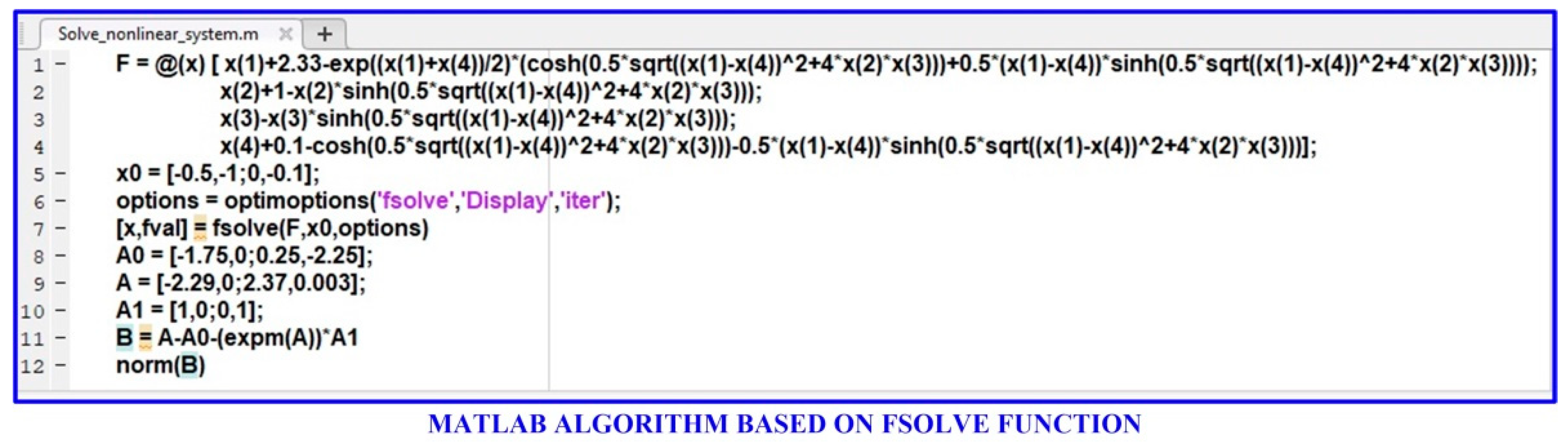
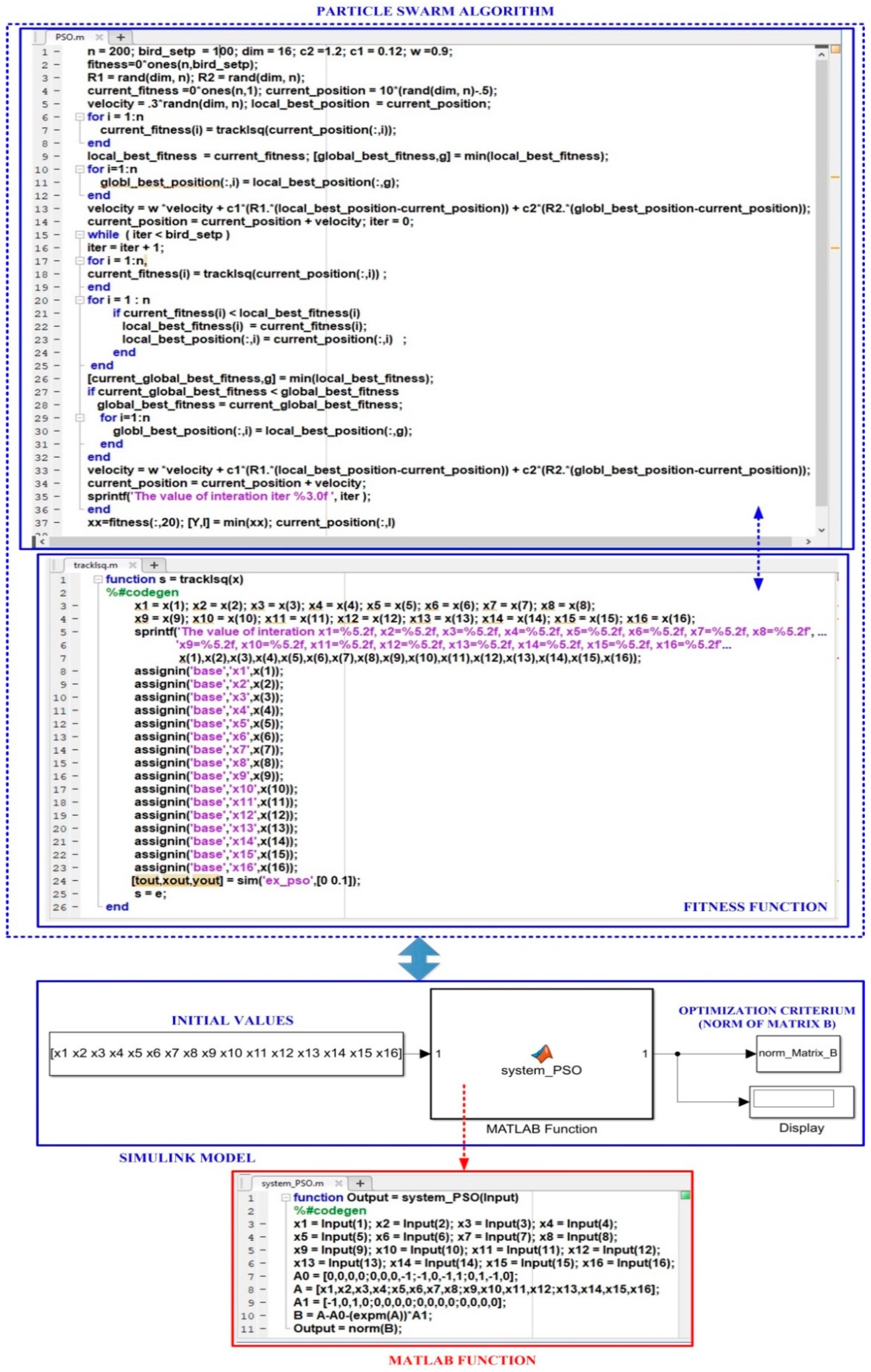
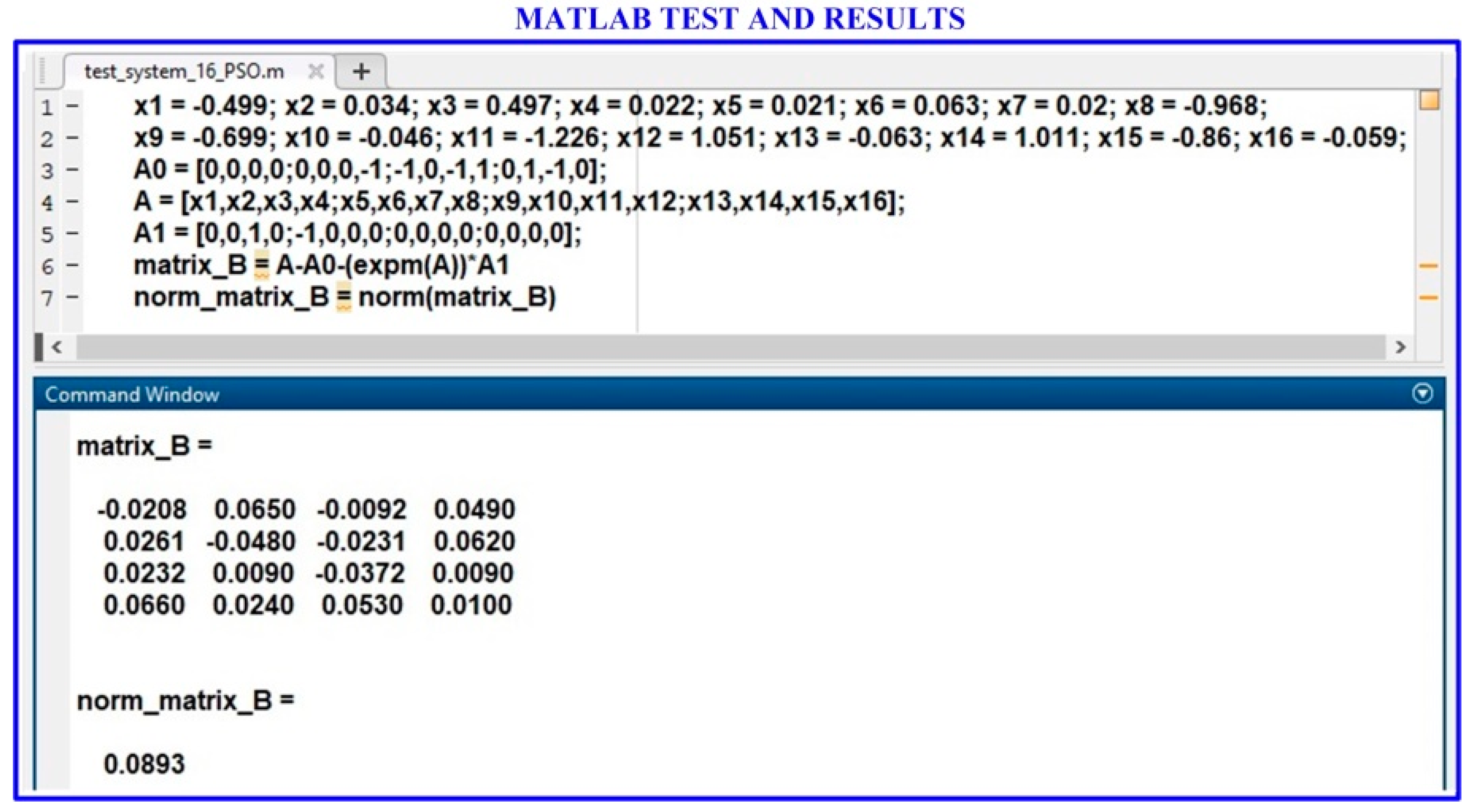
• A numerical solution to the transcendental matrix equation $A=A_0+e^{-Ah}{A}_1$ using the computational-intelligence PSO algorithm.

The article is organized as follows. Section 2 presents some results on the stability of systems with input saturation. Section 3 deals with systems with input saturation and input delay and state delay and presents the steps for obtaining a control law using a general linear transformation. Section 4 presents our main results concerning the sufficient conditions for the global asymptotic stability of systems with input saturation and delay. Numerical examples are provided in Section 5, to illustrate the design procedure for the theoretical results. The conclusions are presented in Section 6.

2. Systems with Saturation in Command

Throughout this article, the described systems are included in the input-state description formalism. In this case, the input of the system is represented by the command applied to it. We considered the single input system:

$$\dot{x}(t)=Ax(t)+B{u}_s(t)$$

(1)

where: $x\in {\Re }^n$ is the state, $u_s\in {\Re }^1$ is the input (command of the system), and $A\in {\Re }^{nxn}$ and $B\in {\Re }^{nx1}$ are matrices of appropriate dimensions.

The command of this system contains saturation and is expressed in the following form:

$$u_s(t)=-sat(Kx)=-\mu (x(t))Kx(t)$$

(2)

where:

$$\mu (x)=\{\begin{array}{ccccc}1& & if& & \left|Kx\right|<u_{\lim }\\ \frac{u_{\lim }}{\left|Kx\right|}& & if& & \left|Kx\right|\ge u_{\lim }\end{array}$$

(3)

where: u_lim is the maxim value of command, $\left|u_s\right|\le u_{\lim }$, and K is a feedback matrix.

We present in this section a set of results from control with a saturation framework [40,41].

Definition 1.

Consider $A_i\in {\Re }^{nxn}$. A set $\{A_1,\dots ,A_k\}$ is simultaneously P Lyapunov stable, if there is a $P\in {\Re }^{nxn}$ positive definite, whereby $A_i^{T}P+P{A}_i<0,\hspace{0.17em}\hspace{0.17em}\hspace{0.17em}\hspace{0.17em}i=1,\dots ,k$.

Theorem 1.

The null solution of closed-loop system (1), (2), and (3) is globally asymptotically stable if there is K and $P\in {\Re }^{nxn}$ positive definite, whereby the set $\left\{A,A-BK\right\}$ is simultaneously P Lyapunov stable, namely: $A^{T}P+PA<0$ and ${(A-BK)}^{T}P+P(A-BK)<0$ [40,41].

Proof of Theorem 1.

Consider the Lyapunov function: $V(x)=x^{T}Px$ and the matrix $P>0$ that fulfills the hypothesis. This results in the following:

$x^T(A^{T}P+PA)x=-x^{T}Qx<0$ and $x^T({(A-BK)}^{T}P+P(A-BK))x=-x^{T}Qx+x^{T}Mx<0$,

where Q > 0 and $M=-(PBK+K^T{B}^{T}P)$.

Then, we obtain $x^{T}Mx<x^{T}Qx$. As $\mu (x)\in (0,1]$, consequently:

$\dot{V}(x)=-x^{T}Qx+\mu (x)x^{T}Mx<-x^{T}Qx+\mu (x)x^{T}Qx\le -x^{T}Qx+x^{T}Qx=0$, and the proof of Theorem 1 is finished [40,41]. □

Definition 2.

Two diagonalizable matrices $A,B\in {\Re }^{nxn}$ are considered to be simultaneously diagonalizable if there is a single non-singular matrix N whereby $N^{-1}AN$ and $N^{-1}BN$ are both diagonal.

Lema 1.

Let A and B be diagonalizable from ${\Re }^{n\times n}$. Then, A and B are simultaneously diagonalizable if and only if A and B commute under multiplication, namely, AB = BA [42].

Theorem 2.

The null solution of closed-loop systems (1), (2), and (3) is globally asymptotically stable if the following are true [40,41]:

1.

The open-loop system A is exponentially stable and diagonalizable;

2.

The matrix $A-BK$ is exponentially stable and diagonalizable;

3.

The matrices A and BK commute under multiplication.

Proof of Theorem 2.

Since A and BK commute, then A and $A-BK$ commute. By assumption, A and $A-BK$ are also diagonalizable.

Thus, according to Lema 1, A and $A-BK$ are simultaneously diagonalizable.

Thus, there is a coordinate transformation T whereby A and $A-BK$ are both diagonal with respect to a new coordinate $z=Tx$.

Let $\overline{A}=A-BK$ and let ${\Lambda }_A, {\Lambda }_{\overline{A}}$ be diagonal matrices where:

$${\Lambda }_A=TA{T}^{-1}, {\Lambda }_{\overline{A}}=T\left(A-BK\right)T^{-1}.$$

Then, we prove that $P=T^{T}T$ satisfies the conditions of Theorem 1.

$2{\Lambda }_A=TA{T}^{-1}+{\left(TA{T}^{-1}\right)}^T$, and by multiplying the left side by T^T and the right side by T, we obtain:

$2T^T{\Lambda }_{A}T=T^T\left(TA{T}^{-1}+{(TA{T}^{-1})}^T\right)T=T^{T}TA+A^T{T}^{T}T=PA+A^{T}P$, where $P=T^{T}T>0$ and $T^T{\Lambda }_{A}T<0$ since T is non-singular.

Similarly: $2T^T{\Lambda }_{\overline{A}}T=T^{T}T\overline{A}+{\overline{A}}^T{T}^{T}T$. Thus, P simultaneously satisfies $A^{T}P+PA<0$ and ${\overline{A}}^{T}P+P\overline{A}<0$. The stability is invariant under change of coordinates, and, by Theorem 1, the proof of Theorem 2 is finished [40,41]. □

Theorem 3.

The null solution of closed-loop systems (1), (2), and (3) is globally asymptotically stable if the following are true [40,41]:

1.

A and $A-BK$ are exponentially stable;

2.

$A-BK$ is diagonalizable;

3.

$\stackrel{⌢}{A}$ commutes with P, where $\stackrel{⌢}{A}$ is the diagonal form of $A-BK$ and $P>0$ solve: $A^{T}P+PA<0$.

Proof of Theorem 3.

Consider $\stackrel{⌢}{A}=T(A-BK)T^{-1}$ where T diagonalizes $A-BK$ and $\stackrel{⌢}{A}$ is diagonal in the new coordinate $z=Tx$ .

Consider also $\overline{A}=TA{T}^{-1}$. Since $\overline{A}$ is exponentially stable, there is $P>0$ that fulfills the hypothesis 3 whereby ${\overline{A}}^{T}P+P\overline{A}<0$.

Since $\stackrel{⌢}{A}<0$ and $P>0$, all eigenvalues of $\stackrel{⌢}{A}P$ are less than zero.

Additionally, the assumption 3 $\stackrel{⌢}{A}P=P\stackrel{⌢}{A}$ and ${\stackrel{⌢}{A}}^T=\stackrel{⌢}{A}$ implies that ${\stackrel{⌢}{A}}^{T}P+P\stackrel{⌢}{A}<0$. The stability is invariant under change of coordinate, and, by Theorem 1, the proof of Theorem 3 is finished [40,41]. □

Theorem 4.

We consider the multiple-input system in the following form [40,41]:

$$\dot{x}=Ax+B{u}_s=Ax+{\displaystyle \sum _{i=1}^m{B}_i{u}_{si}}$$

(4)

where: $x\in {\Re }^n,u_s\in {\Re }^m,A\in {\Re }^{nxn}$ is asymptotically stable, $B\in {\Re }^{nxm}$, B_i is the i-th column of B.

The command contains saturation and is expressed in the following form: $u_s={\left[\begin{array}{ccc}{u}_{s1},& \dots & ,u_{sm}\end{array}\right]}^T$, where $u_{\max \hspace{0.17em}i}$ is the maxim value of the component i-th of command, namely: $\left|u_{si}\right|<u_{\max i},i=1,\dots ,m$.

The components of the command vector $u_s=-sat(B^{T}Py)$ are expressed in the following form:

$$u_{si}=\{\begin{array}{l}-B_i^{T}Px if \left|B_i^{T}Px\right|<u_{\max \hspace{0.17em}i}\\ -{\mu }_i{B}_i^{T}Px if \left|B_i^{T}Px\right|\ge u_{\max \hspace{0.17em}i}\end{array}$$

(5)

where:

$${\mu }_i=\frac{u_{\max i}}{\left|B_i^{T}Px\right|}\hspace{1em}i=1,\dots ,m$$

(6)

If $P>0$ solves $A^{T}P+PA<0$, then the null solution of closed-loop systems (4), (5), and (6) is globally asymptotically stable.

Proof of Theorem 4.

We can rewrite the command vector: $u_s=-M{B}^{T}Px$,

where: $M=diag({\beta }_i),M\in {\Re }^{mxm},{\beta }_i\in (0,1]$ and ${\beta }_i=\{\begin{array}{ccccc}1& & if& & \left|B_i^{T}Px\right|<u_{\max i}\\ {\mu }_i& & if& & \left|B_i^{T}Px\right|\ge u_{\max i}\end{array}$.

Consider the Lyapunov function: $V(x)=x^{T}Px$ and by computing $\dot{V}(x)$, we obtain: $\dot{V}(x)=x^T[{(A-BM{B}^{T}P)}^{T}P+P(A-BM{B}^{T}P)]x=x^T(A^{T}P+PA-2PBM{B}^{T}P)x<0$, since $PBM{B}^{T}P\ge 0$ and $A^{T}P+PA<0$. Thus, the proof of Theorem 4 is finished [40,41]. □

Theorem 5.

We consider system (1) and suppose A is invertible and has a single unstable eigenvalue λ.

Let $x_{eq}=\pm A^{-1}B{u}_{\lim }$ denote the equilibrium points of the saturated system when the input saturates at $u_s=-u_{\lim }$ and $u_s=u_{\lim }$, respectively.

Then, no feedback matrix K, where $\left|K{x}_{eq}\right|\ge u_{\lim }$, can globally stabilize the null solution of closed-loop systems (1), (2), and (3) [40,41].

Proof of Theorem 5.

To show that the origin is not globally asymptotically stable, it is sufficient to find some initial conditions $x_0\in {\Re }^n$ that cannot be driven to the origin with the feedback control law: $u_s(t)=-sat(Kx)=-\mu (x(t))Kx(t)$ where K fulfills: $\left|K{x}_{eq}\right|\ge u_{\lim }$.

Let $E_{\lambda }(x_{eq})$ be the eigenspace corresponding to the unstable eigenvalue λ of the open-loop system A, where $E_{\lambda }(x_{eq})=\left\{x\in {\Re }^n:\hspace{0.17em}\hspace{0.17em}A(x-x_{eq})=\lambda (x-x_{eq})\right\}$.

We show that some initial conditions on the eigenspace $E_{\lambda }$ cannot be driven to the origin with the feedback $u_s(t)=-sat(Kx)$.

Note that $\left|Kx\right|=u_{\lim }$ depicts the saturation boundaries. Now consider the case when saturation occurs with $u_s=-u_{\lim }$.

Then, the dynamics of the saturated system are given by: $\dot{x}(t)=Ax(t)-B{u}_{\lim }$ and the equilibrium point under saturation by $x_{eq}=A^{-1}B{u}_{\lim }$.

Consider $D=\left\{x\hspace{0.17em}\hspace{0.17em}:\hspace{0.17em}\hspace{0.17em}\left|Kx\right|\ge u_{\lim }\right\}$. The assumption $\left|K{x}_{eq}\right|\ge u_{\lim }$ implies $x_{eq}\in D$. Then, the trajectory $x(t)$ for the saturated system when $x_0\in E_{\lambda }(x_{eq})$ is given by $x(t)=e^{\lambda t}(x_0-x_{eq})+x_{eq}$.

Moreover, since $E_{\lambda }(x_{eq})$ is the eigenspace, $x(t)\in E_{\lambda }(x_{eq})\cap D$ provided the system remains saturated at $u_s=-u_{\lim }$.

We show that some initial conditions $x_0\in E_{\lambda }\cap D$ exist where $x(t)$ never leaves the saturated region D so that $\left|x(t)\right|$ becomes unbounded.

Now $E_{\lambda }$ is either parallel to or intersects $Kx=u_{\lim }$. Because $Kx=u_{\lim }$ forms an $n-1$ dimensional surface and $Ex(x_{eq})$ a line, the intersection is a point. Suppose $E_{\lambda }(x_{eq})$ and $Kx=u_{\lim }$ are parallel. Since $x_{eq}\in D$, $E_{\lambda }(x_{eq})$ is entirely situated in the saturated region, this means that: $\forall x_0\in E_{\lambda }(x_{eq}),\hspace{0.17em}x(t)\in E_{\lambda }(x_{eq}),\hspace{0.17em}\hspace{0.17em}\forall t\ge 0$. Since $E_{\lambda }(x_{eq})$ is an unstable eigenspace, $\left|x(t)\right|$ will become unbounded. Now suppose $E_{\lambda }(x_{eq})$ and $Kx=u_{\lim }$ intersect. Let $v^{*}$ denote the point of intersection. Then, $\forall x_0\in E_{\lambda }(x_{eq})\cap D$ whereby $\left|x_0\right|\ge \max \left(\left|v^{*}\right|\hspace{0.17em},\hspace{0.17em}\left|x_{eq}\right|\right)$, $x(t)\in E_{\lambda }(x_{eq})\cap D,\hspace{0.17em}\hspace{0.17em}t\ge 0$, and $\left|x(t)\right|$ will become unbounded.

The same argument can be repeated for saturation occurring at $u_s=u_{\lim }$.

Thus, there exist initial conditions on the eigenspace corresponding to the unstable eigenvalue λ, which make the states unbounded.

Hence, the origin is not globally asymptotically stable under any linear time-invariant state feedback, and the proof of Theorem 5 is finished [40,41]. □

Theorem 6.

We consider system (1) and assume the following as true [40,41]:

1.

Matrix A is unstable;

2.

Matrix $A-BK$ is exponentially stable.

Consider $B_d=\left\{x\hspace{0.17em}\hspace{0.17em}:x^{T}Px\le d\right\}$,$\hspace{0.17em}d\in {\Re }_{+}$, and $H=\left\{x\hspace{0.17em}\hspace{0.17em}:\hspace{0.17em}\hspace{0.17em}\left|Kx\right|\le u_{\lim }\right\}$, where $P>0$ is a solution to ${(A-BK)}^{T}P+P(A-BK)<0$.

Then, $B_{d^{*}}^{}$ is an exponentially stable region for the closed-loop systems (1), (2), and (3), where $d^{*}$ is the largest number whereby $B_{d^{*}}^{}\subset H$.

Proof of Theorem 6.

Since $A-BK$ is exponentially stable, there is the matrix $P>0$, whereby: ${(A-BK)}^{T}P+P(A-BK)<0$.

For $\forall x\in H$, $u_s(t)=-sat(Kx)=-Kx(t)$ and consider the Lyapunov function: $V(x)=x^{T}Px$, and by computing $\dot{V}(x)$ we obtain:

$$\dot{V}(x)=x^T[{(A-BK)}^{T}P+P(A-BK)]x<0.$$

In addition, $B_{d^{*}}$ is the largest set that is situated within the unsaturated region H. Thus, $\forall x\in B_{d^{*}}$, $x^{T}Px$ decreases and hence $\left|x\right|\to 0$ exponentially. Thus, the proof of Theorem 6 is finished [40,41]. □

3. Systems with Command Saturation, Saturation Delay, and State Delay

3.1. Systems with Point Delays

In first part of this section, we consider the system with point delay (S_d) in the following form:

$$\dot{x}(t)=A_{0}x(t)+A_{1}x(t-h)+B_0{u}_s(t)+B_1{u}_s(t-h)$$

(7)

where: $x\in {\Re }^n$ is the state, $u_s\in {\Re }^m$, h is the input delay and state delay (we consider the same state delay and input delay and a single delay just for easy writing), and $A_0, A_1, B_0, B_1$ are matrices of appropriate dimensions.

The initial command conditions are given by a function $u_{s0}(\cdot )$ defined for the interval $[-h,0]$, and the initial state condition is given by a function $x_0(\cdot )$ defined for the interval $[-h,0]$.

The command u_s contains saturation and $\left|u_s\right|\le u_{\lim }$ where $u_{\lim }$ is the maxim value of command in the single-input case.

In the multiple-input case, the command contains saturation and is expressed in the following form: $u_s={\left[\begin{array}{ccc}{u}_{s1},& \dots & ,u_{sm}\end{array}\right]}^T$, $u_{\max \hspace{0.17em}i}$ is the maxim value of the component i-th of the command, namely: $\left|u_{si}\right|<u_{\max i},i=1,\dots ,m$.

Consider system (4), using the state transformation:

$$\tilde{y}(t)=x(t)+{\displaystyle \underset{t-h}{\overset{t}{\int }}{e}^{(t-s-h)A}{A}_{1}x(s)ds}+{\displaystyle \underset{t-h}{\overset{t}{\int }}{e}^{(t-s-h)A}{B}_1{u}_s(s)ds}$$

(8)

where: A is a solution of the transcendental matrix equation:

$$A=A_0+e^{-Ah}{A}_1$$

(9)

We note $s=t+\theta$, and, by computing $\dot{\tilde{y}}$, we obtain:

$$\begin{gathered} \dot{\tilde{y}}(t)=A_{0}x(t)+A_{1}x(t-h)+B_0{u}_s(t)+B_1{u}_s(t-h)+{\displaystyle \underset{-h}{\overset{0}{\int }}{e}^{-A(\theta +h)}{A}_1\dot{x}(t+\theta )d\theta }+{\displaystyle \underset{-h}{\overset{0}{\int }}{e}^{-A(\theta +h)}{B}_1{\dot{u}}_s(t+\theta )d\theta } \\ \begin{array}{l}{\displaystyle \underset{-h}{\overset{0}{\int }}{e}^{-A(\theta +h)}{A}_1\dot{x}(t+\theta )d\theta =e^{-A(\theta +h)}{A}_{1}x(t+\theta ){|}_{-h}^0+}{\displaystyle \underset{-h}{\overset{0}{\int }}A{e}^{-A(\theta +h)}{A}_{1}x(t+\theta )d\theta }\\ =e^{-Ah}{A}_{1}x(t)-A_{1}x(t-h)+{\displaystyle \underset{-h}{\overset{0}{\int }}A{e}^{-A(\theta +h)}{A}_{1}x(t+\theta )d\theta }\end{array} \\ \begin{array}{l}{\displaystyle \underset{-h}{\overset{0}{\int }}{e}^{-A(\theta +h)}{B}_1{\dot{u}}_s(t+\theta )d\theta =e^{-A(\theta +h)}{B}_1{u}_s(t+\theta ){|}_{-h}^0+}{\displaystyle \underset{-h}{\overset{0}{\int }}A{e}^{-A(\theta +h)}{B}_1{u}_s(t+\theta )d\theta }\\ =e^{-Ah}{B}_1{u}_s(t)-B_1{u}_s(t-h)+{\displaystyle \underset{-h}{\overset{0}{\int }}A{e}^{-A(\theta +h)}{B}_1{u}_s(t+\theta )d\theta }\end{array} \end{gathered}$$

Noting that the sum formed by the last integral of each term above is equal to $A(\tilde{y}(t)-x(t))$, using (9) and making the replacement above, we obtain the associated system:

$$\dot{\tilde{y}}(t)=A\tilde{y}(t)+(B_0+e^{-hA}{B}_1)u_s(t)$$

(10)

We make the following notation:

$$B=B_0+e^{-hA}{B}_1$$

(11)

System (7), with (6) and (8), is called the associate system of (4) and becomes:

$$\dot{\tilde{y}}(t)=A\tilde{y}(t)+B{u}_s(t)$$

(12)

where: $\tilde{y}\in {\Re }^n$ is the state, and A and B represent the matrices of appropriate dimensions.

The command of this system contains saturation, and in the single input case it is expressed in the following form:

$$u_s(t)=-sat(K\tilde{y})=-\mu (\tilde{y}(t))K\tilde{y}(t)$$

(13)

where:

$$\mu (\tilde{y})=\{\begin{array}{ccccc}1& & if& & \left|K\tilde{y}\right|<u_{\lim }\\ \frac{u_{\lim }}{\left|K\tilde{y}\right|}& & if& & \left|K\tilde{y}\right|\ge u_{\lim }\end{array}$$

(14)

where: $u_{\lim }$ is the maxim value of command, and $\left|u_s\right|\le u_{\lim }$, K is a feedback matrix.

The unstable poles for system (7) are given by ${\Lambda }_{\mathrm{c}}=\left\{s:\det \left(sI-A_0-e^{-hs}{A}_1\right)=0,\hspace{0.17em}\hspace{0.17em}\mathrm{Re}(s)\ge -{\upsilon }_0\right\}$, where ${\upsilon }_0\ge 0$ is the desired margin of stability. System (7) is ${\upsilon }_0$, and is stabilizable if and only if: $rank[sI-A_0-e^{-hs}{A}_1|B_0+e^{-hs}{B}_1]=n$, for all $s\in C_{-{\upsilon }_0}^{+}=\left\{s\in C:\hspace{0.17em}\mathrm{Re}(s)\ge -{\upsilon }_0\right\}$.

We note $\Gamma =\left\{A\in C^{nxn}:A=A_0+e^{-Ah}{A}_1\right\}$. Then, $\forall A\in \Gamma ,\hspace{0.17em}\hspace{0.17em}\hspace{0.17em}\sigma (A)\subset \sigma (S_d)={\Lambda }_c$ [37,38,39].

With these, the stabilizability of (S_d) implies complete controllability of the associated system without delay (12). Equation (9) plays a key role for obtaining system (12) without delay. In the general case, the unstable poles of system (7) are given by ${\Lambda }_c$, which comprise $nN$ elements (augmented as necessary with the stable poles); N is a positive integer and thereby allows the following representation:

$${\Lambda }_c={\Lambda }_1\cup {\Lambda }_2\cup \dots \cup {\Lambda }_N$$

(15)

where: ${\Lambda }_i,\hspace{0.17em}i=\overline{1,N}$ is a symmetric set of cardinality n.

For every set ${\Lambda }_i=\left\{s_1,s_2,\dots ,s_n\right\}$, we consider the eigenvalues—even the unstable poles in the Jordan matrix: $J=diag\left[s_1,s_2,\dots ,s_n\right]$.

If ${\Lambda }_i$ has complex conjugate elements $s_k={\sigma }_0\pm j{\omega }_0$, then the corresponding Jordan cell is expressed in the following form: $J_k=\left[\begin{array}{cc}{\sigma }_0& -{\omega }_0\\ {\omega }_0& {\sigma }_0\end{array}\right]$.

Additionally, we consider the corresponding set $\left\{w_1,w_2,\dots ,w_n\right\}$ of right eigenvectors arranged as a modal matrix $P=\left[w_1,w_2,\dots ,w_n\right]$, where each pair $(s_k,w_k)$ fulfills the equation:

$$\left(s_{k}I-A_0-e^{-h{s}_k}{A}_1\right)w_k=0,\hspace{0.17em}{s}_k\in {\Lambda }_c$$

(16)

The matrix $A_{ci}=PJ{P}^{-1}$ fulfills Equation (9).

In a similar way, for a set of n left eigenvectors $\left\{v_1,v_2,\dots ,v_n\right\}$ fulfilling the equation:

$$\left(s_{k}I-A_0-e^{-h{s}_k}{A}_1\right)w_k=0,\hspace{0.17em}{s}_k\in {\Lambda }_c$$

(17)

Consider the matrix $Q=col\left[v_1,v_2,\dots ,v_n\right]$; then, the matrix $A_{ci}=Q^{-1}JQ$ fulfills Equation (9).

When $N\ge 2$, the solution of (9) is:

$$\left(s_{k}I-A_0-e^{-h{s}_k}{A}_1\right)w_k=0,\hspace{0.17em}{s}_k\in {\Lambda }_c$$

(18)

The matrix $B_c=B$ fulfills (11), but the matrices B₀ and B₁ are now $B_0=col\left[B_0,\dots ,B_0\right]\in R^{nNx1}$ and $B_1=col\left[B_1,\dots ,B_1\right]\in R^{nNx1}$, respectively.

The stabilizing feedback matrix K is now:

$K_c=row\left[K_1,\dots ,K_N\right]$ whereby the matrix $\left(A_c-B_c{K}_c\right)$ is Hurwitzian with the desired ${\upsilon }_0\ge 0$ degree of stability.

From the systems with delay, the next result is well known [37,38,39].

Proposition 1.

If $u(t)=F(\cdot )\tilde{y}(t)$ is a stabilizing control law for the associated system (12), then the next control law:

$$u(t)=F(\cdot )[x(t)+{\displaystyle \underset{-h}{\overset{0}{\int }}{e}^{-A(\theta +h)}{A}_{1}x(t+\theta )d\theta }+{\displaystyle \underset{-h}{\overset{0}{\int }}{e}^{-A(\theta +h)}{B}_1{u}_s(t+\theta )d\theta }]$$

(19)

is stabilizing for system (7), under the condition that all unstable eigenvalues of system (7) are contained in the spectrum of the matrix A given by (9).

In our case, for $F(\cdot )=-\mu (\tilde{y})K$, the command of (7) contains saturation, and it is expressed in the following form:

$$\begin{array}{ll}{u}_s(t)=& -\mu (x(t)+{\displaystyle \underset{-h}{\overset{0}{\int }}{e}^{-A(\theta +h)}{A}_{1}x(t+\theta )d\theta }+{\displaystyle \underset{-h}{\overset{0}{\int }}{e}^{-A(\theta +h)}{B}_1{u}_s(t+\theta )d\theta })K[x(t)\\ & +{\displaystyle \underset{-h}{\overset{0}{\int }}{e}^{-A(\theta +h)}{A}_{1}x(t+\theta )d\theta }+{\displaystyle \underset{-h}{\overset{0}{\int }}{e}^{-A(\theta +h)}{B}_1{u}_s(t+\theta )d\theta }]\end{array}$$

(20)

where the matrix A is given by (9) and:

$$\begin{array}{l}\mu (x+{\displaystyle \underset{-h}{\overset{0}{\int }}{e}^{-A(\theta +h)}{A}_{1}x(t+\theta )d\theta }+{\displaystyle \underset{-h}{\overset{0}{\int }}{e}^{-A(\theta +h)}{B}_1{u}_s(t+\theta )d\theta })=1\hspace{0.17em}\\ if\hspace{0.17em}\\ \hspace{0.17em}\left|K(x+{\displaystyle \underset{-h}{\overset{0}{\int }}{e}^{-A(\theta +h)}{A}_{1}x(t+\theta )d\theta }+{\displaystyle \underset{-h}{\overset{0}{\int }}{e}^{-A(\theta +h)}{B}_1{u}_s(t+\theta )d\theta })\right|<u_{\lim }\\ \mu (x+{\displaystyle \underset{-h}{\overset{0}{\int }}{e}^{-A(\theta +h)}{A}_{1}x(t+\theta )d\theta }+{\displaystyle \underset{-h}{\overset{0}{\int }}{e}^{-A(\theta +h)}{B}_1{u}_s(t+\theta )d\theta })=\\ =\frac{u_{\lim }}{\left|K(x+{\displaystyle \underset{-h}{\overset{0}{\int }}{e}^{-A(\theta +h)}{A}_{1}x(t+\theta )d\theta }+{\displaystyle \underset{-h}{\overset{0}{\int }}{e}^{-A(\theta +h)}{B}_1{u}_s(t+\theta )d\theta })\right|}\\ if\\ \left|K(x+{\displaystyle \underset{-h}{\overset{0}{\int }}{e}^{-A(\theta +h)}{A}_{1}x(t+\theta )d\theta }+{\displaystyle \underset{-h}{\overset{0}{\int }}{e}^{-A(\theta +h)}{B}_1{u}_s(t+\theta )d\theta })\right|\ge u_{\lim }\end{array}$$

(21)

$u_{\lim }$ is the maxim value of the command, $\left|u_s\right|\le u_{\lim }$, and K is a feedback matrix.

When $N\ge 2$, the control law (19) becomes:

$$u(t)=-\left[{\displaystyle \sum _{i=1}^N{K}_i}\right]x(t)-{\displaystyle \underset{-h}{\overset{0}{\int }}\left[{\displaystyle \sum _{i=1}^N{K}_i{e}^{-A_{ci}(\theta +h)}}\right]}{A}_{1}x(t+\theta )d\theta -{\displaystyle \underset{-h}{\overset{0}{\int }}\left[{\displaystyle \sum _{i=1}^N{K}_i{e}^{-A_{ci}(\theta +h)}}\right]}{B}_{1}u(t+\theta )d\theta$$

(22)

Remark 1.

The general form of the systems with multiple point delays is treated in a similar way.

Consider (S_d) in the following form:

$$\dot{x}(t)=A_{0}x(t)+{\displaystyle \sum _{i=1}^R{A}_{i}x(t-r_i)}+B_0{u}_s(t)+{\displaystyle \sum _{i=1}^H{B}_i{u}_s(t-h_i)}$$

(23)

where $x\in {\Re }^n$ is the state; $u_s\in {\Re }^m$, $h_i,\hspace{0.17em}\hspace{0.17em}i=1,\dots ,H$ are the input delays; $r_i,\hspace{0.17em}\hspace{0.17em}i=1,\dots ,R$ are the state delays; and $A_0, A_i, B_0, B_i$ are matrices of appropriate dimensions.

The initial command conditions are given by a function $u_{s0}(\cdot )$ defined for the interval $[-h,0]$, and the initial state condition is given by a function $x_0(\cdot )$ defined for the interval $[-r,0]$, where: $h=\max \{h_1,\dots ,h_H\}$ and $r=\max \{r_1,\dots ,r_R\}$.

The command contains saturation, and using the state transformation:

$$\tilde{y}(t)=x(t)+{\displaystyle \sum _{i=1}^R{\displaystyle \underset{t-r_i}{\overset{t}{\int }}{e}^{(t-s-r_i)A}{A}_{i}x(s)ds}}+{\displaystyle \sum _{i=1}^H{\displaystyle \underset{t-h_i}{\overset{t}{\int }}{e}^{(t-s-h_i)A}{B}_i{u}_s(s)ds}},$$

(24)

we obtain the associated system without delay expressed in the form (12), where:

$A=A_0+{\displaystyle \sum _{i=1}^R{e}^{-r_{i}A}{A}_i}$ and $B=B_0+{\displaystyle \sum _{i=1}^H{e}^{-h_{i}A}{B}_i}$. If $R=0$, the state transformation (24) is called an Artstein transform [2,37,38,39].

When $N\ge 2$, the control law (22) becomes:

$$u(t)=-\left[{\displaystyle \sum _{i=1}^N{K}_i}\right]x(t)-{\displaystyle \underset{-h}{\overset{0}{\int }}{\displaystyle \sum _{j=1}^R\left[{\displaystyle \sum _{i=1}^N{K}_i{e}^{-A_{ci}(\theta +r_j)}}\right]}}{A}_{j}x(t+\theta )d\theta \hspace{0.17em}-{\displaystyle \underset{-h}{\overset{0}{\int }}{\displaystyle \sum _{j=1}^H\left[{\displaystyle \sum _{i=1}^N{K}_i{e}^{-A_{ci}(\theta +h_j)}}\right]}}{B}_{j}u(t+\theta )d\theta$$

(25)

where: $A, B, A_c, B_c, K_c$ are calculated as in the case of (S_d) expressed by (7).

Remark 2.

If the state vector $x\in {\Re }^n$ is not fully measured, we can use a combined controller/observer. For example, consider system (23) with $R=1,\hspace{0.17em}H=0$; then, the observer is [37]:

$$\dot{\widehat{x}}(t)=A_0\widehat{x}(t)+A_1\widehat{x}(t-r)+B_0{u}_s(t)+L(z(t)-C \widehat{x}(t))+{\displaystyle \underset{-r}{\overset{0}{\int }}{e}^{-A(\theta +r)}}{A}_{1}L(z(t+\theta )-C \widehat{x}(t+\theta ))d\theta$$

(26)

where $z(t)=Cx(t)$ is the output and L is the matrix of the observer.

3.2. Systems with Distributed Delay

In the last part of this section, we consider the system with distributed delay (S_dd) in the following form:

$$\dot{x}(t)={\displaystyle \underset{-h}{\overset{0}{\int }}d\alpha (\theta )x(t+\theta )+{\displaystyle \underset{-h}{\overset{0}{\int }}d\beta (\theta )u_s(t+\theta )}}$$

(27)

where: $x\in {\Re }^n$ is the state, $u_s\in {\Re }^m\hspace{0.17em}$.

$\hspace{0.17em}\alpha \in BV\left(\hspace{0.17em}[-h\hspace{0.17em},\hspace{0.17em}0]\hspace{0.17em},\hspace{0.17em}{\Re }^{nxn}\hspace{0.17em}\right)\hspace{0.17em},\hspace{0.17em}\beta \in BV\left(\hspace{0.17em}[-h\hspace{0.17em},\hspace{0.17em}0]\hspace{0.17em},\hspace{0.17em}{\Re }^{nxm}\right)\hspace{0.17em},\hspace{0.17em}h>0$ is the input delay and state delay. $BV\left(\hspace{0.17em}[-h\hspace{0.17em},\hspace{0.17em}0]\hspace{0.17em},\hspace{0.17em}{\Re }^{n_{1}x{n}_2}\right)$ denotes the class of integrable $n_1\times n_2$ matrix-valued functions of bounded variations. The initial conditions are given by:$x(\theta )=x_0(\theta )\hspace{0.17em}\hspace{0.17em}\hspace{0.17em}\hspace{0.17em}$;$\hspace{0.17em}\hspace{0.17em}{u}_s(\theta )=u_{s0}(\theta )\hspace{0.17em}\hspace{0.17em}\hspace{0.17em}for\hspace{0.17em}\hspace{0.17em}\hspace{0.17em}\theta \in [-h,0]$; $x_0\in C\hspace{0.17em}\left(\hspace{0.17em}[-h\hspace{0.17em},\hspace{0.17em}0]\hspace{0.17em},\hspace{0.17em}{\Re }^n\right)\hspace{0.17em}$,$\hspace{0.17em}{u}_{s0}\in C\hspace{0.17em}\left(\hspace{0.17em}[-h\hspace{0.17em},\hspace{0.17em}0]\hspace{0.17em},\hspace{0.17em}{\Re }^m\right)$.

In the single-input case $m=1$, the command $u_s$ contains saturation and $\left|u_s\right|\le u_{\lim }$ where $u_{\lim }$ is the maxim value of the command.

In the multiple-input case, the command contains saturation and is expressed in the form: $u_s={\left[\begin{array}{ccc}{u}_{s1},& \dots & ,u_{sm}\end{array}\right]}^T$, and $u_{\max \hspace{0.17em}i}$ is the maxim value of the component i-th of command, namely: $\left|u_{si}\right|<u_{\max i},i=1,\dots ,m$.

Consider system (27), and using the state transformation:

$$\tilde{y}(t)=x(t)+{\displaystyle \underset{-h}{\overset{0}{\int }}\hspace{0.17em}{\displaystyle \underset{t+\theta }{\overset{t}{\int }}{e}^{A(t+\theta -\tau )}}d\alpha (\theta )x(\tau )d\tau }+{\displaystyle \underset{-h}{\overset{0}{\int }}\hspace{0.17em}{\displaystyle \underset{t+\theta }{\overset{t}{\int }}{e}^{A(t+\theta -\tau )}d\beta (\theta )u_s(\tau )d\tau }}$$

(28)

where: A is a solution of the transcendental matrix equation:

$$A={\displaystyle \underset{-h}{\overset{0}{\int }}{e}^{A\theta }d\alpha (\theta )}$$

(29)

The associated system for (27) is:

$$\dot{\tilde{y}}(t)=A\tilde{y}(t)+B{u}_s(t)$$

(30)

where:

$$B={\displaystyle \underset{-h}{\overset{0}{\int }}{e}^{A\theta }d\beta (\theta )}$$

(31)

We obtain the associated system (30) if we note: $s=t+\theta$, and by computing $\dot{\tilde{y}}$:

$$\begin{array}{l}\dot{\tilde{y}}(t)={\displaystyle \underset{-h}{\overset{0}{\int }}d\alpha (\theta )x(t+\theta )}+{\left({\displaystyle \underset{-h}{\overset{0}{\int }}\hspace{0.17em}{\displaystyle \underset{t+\theta }{\overset{t}{\int }}{e}^{A(t+\theta -\tau )}}d\alpha (\theta )x(\tau )d\tau }\right)}^{\prime }+\\ {\displaystyle \underset{-h}{\overset{0}{\int }}d\beta (\theta )u_s(t+\theta )}+{\left({\displaystyle \underset{-h}{\overset{0}{\int }}\hspace{0.17em}{\displaystyle \underset{t+\theta }{\overset{t}{\int }}{e}^{A(t+\theta -\tau )}d\beta (\theta )u_s(\tau )d\tau }}\right)}^{\prime }.\end{array}$$

Using (26) and (28), we can write:

$$\begin{array}{l}{\left({\displaystyle \underset{-h}{\overset{0}{\int }}\hspace{0.17em}{\displaystyle \underset{t+\theta }{\overset{t}{\int }}{e}^{A(t+\theta -\tau )}}d\alpha (\theta )x(\tau )d\tau }\right)}^{\prime }=A{\left\{{\displaystyle \underset{t+\theta }{\overset{t}{\int }}{e}^{A(t-\tau )}}x(\tau )d\tau \right\}}^{\prime }=\\ Ax(t)-A{e}^{-A\theta }x(t+\theta )+A{\displaystyle \underset{t+\theta }{\overset{t}{\int }}A{e}^{A(t-\tau )}}x(\tau )d\tau \mathrm{and}\\ {\left({\displaystyle \underset{-h}{\overset{0}{\int }}\hspace{0.17em}{\displaystyle \underset{t+\theta }{\overset{t}{\int }}{e}^{A(t+\theta -\tau )}}d\beta (\theta )u_s(\tau )d\tau }\right)}^{\prime }=B{\left\{{\displaystyle \underset{t+\theta }{\overset{t}{\int }}{e}^{A(t-\tau )}}{u}_s(\tau )d\tau \right\}}^{\prime }=\\ B{u}_s(t)-B{e}^{-A\theta }{u}_s(t+\theta )+B{\displaystyle \underset{t+\theta }{\overset{t}{\int }}A{e}^{A(t-\tau )}}{u}_s(\tau )d\tau .\end{array}$$

Noting that the sum formed by the last integral of each term above is equal to $A(\tilde{y}(t)-x(t))$, using (28), (29), and (31), making the replacement above, we obtain the associated system (30). The command of this system contains saturation, and in the single-input case it is expressed in the following form:

$$u_s(t)=-sat(K\tilde{y})=-\mu (\tilde{y}(t))K\tilde{y}(t)$$

(32)

where:

$$\mu (\tilde{y})=\{\begin{array}{ccccc}1& & if& & \left|K\tilde{y}\right|<u_{\lim }\\ \frac{u_{\lim }}{\left|K\tilde{y}\right|}& & if& & \left|K\tilde{y}\right|\ge u_{\lim }\end{array}$$

(33)

where: $u_{\lim }$ is the maxim value of the command, and $\left|u_s\right|\le u_{\lim }$, K is a feedback matrix.

The unstable poles for system (27) are given by:

${\Lambda }_{\mathrm{c}}=\left\{s:\det \left(sI-{\displaystyle \underset{-h}{\overset{0}{\int }}{e}^{s\theta }d\alpha (\theta )}\right)=0,\hspace{0.17em}\hspace{0.17em}\mathrm{Re}(s)\ge -{\upsilon }_0\right\}$, where ${\upsilon }_0\ge 0$ is the desired margin of stability.

System (24) is ${\upsilon }_0$—stabilizable if and only if:

$rank\left[sI-{\displaystyle \underset{-h}{\overset{0}{\int }}{e}^{s\theta }}d\alpha (\theta )|{\displaystyle \underset{-h}{\overset{0}{\int }}{e}^{s\theta }}d\beta (\theta )\right]=n$, for all $s\in C_{-{\upsilon }_0}^{+}=\left\{s\in C:\hspace{0.17em}\mathrm{Re}(s)\ge -{\upsilon }_0\right\}$.

We note $\Gamma =\left\{A\in C^{nxn}:A={\displaystyle \underset{-h}{\overset{0}{\int }}{e}^{A\theta }}d\alpha (\theta )\right\}$. Then, $\forall A\in \Gamma ,\hspace{0.17em}\hspace{0.17em}\hspace{0.17em}\sigma (A)\subset \sigma (S_d)={\Lambda }_c$—see [34,35].

With these, the stabilizability of (S_dd) implies complete controllability of the associated system without delay (30).

Equation (29) plays a key role for obtaining system (30) with no delay.

Similarly to the case of the point-delay system, an algorithm was developed in [34,35] for solving Equation (29). The spectrum of (S_dd) is ${\Lambda }_c$, which allows the following representation:

$${\Lambda }_c={\Lambda }_1\cup {\Lambda }_2\cup \dots \cup {\Lambda }_N$$

(34)

where: ${\Lambda }_i,\hspace{0.17em}i=\overline{1,N}$ is a symmetric set of cardinality n.

For every set ${\Lambda }_i=\left\{s_1,s_2,\dots ,s_n\right\}$, we consider the matrix $J=diag\left[s_1,s_2,\dots ,s_n\right]$ of eigenvalues s_k of the matrix:

$$A_{s_k}={\displaystyle \underset{-h}{\overset{0}{\int }}{e}^{s_k\theta }}d\alpha (\theta )$$

(35)

Additionally, we consider the corresponding set $\left\{v_1,v_2,\dots ,v_n\right\}$ of left eigenvectors (or, in a similar way, the right eigenvectors) arranged as a matrix $Q=col\left[v_1,v_2,\dots ,v_n\right]$, where each pair $(s_k,v_k)$ fulfills the equation:

$$v_k\left(s_{k}I-{\displaystyle \underset{-h}{\overset{0}{\int }}{e}^{s_k\theta }}d\alpha (\theta )\right)=0,\hspace{0.17em}{s}_k\in {\Lambda }_i$$

(36)

then, the matrix $A_{ci}=Q^{-1}JQ$, fulfills the Equation (29), and the general solution is:$A_c=diag\left[A_{c1},A_{c2},\dots ,A_{cN}\right]$.

From the systems with distributed delay, the next result is well known [34,35].

Proposition 2.

If $u(t)=F(\cdot )\tilde{y}(t)$ is a stabilizing law for associated system (30), then the next control law:

$$u(t)=F(\cdot )\left[x(t)+{\displaystyle \underset{-h}{\overset{0}{\int }}\hspace{0.17em}{\displaystyle \underset{t+\theta }{\overset{t}{\int }}{e}^{A(t+\theta -\tau )}}d\alpha (\theta )x(\tau )d\tau }+{\displaystyle \underset{-h}{\overset{0}{\int }}\hspace{0.17em}{\displaystyle \underset{t+\theta }{\overset{t}{\int }}{e}^{A(t+\theta -\tau )}d\beta (\theta )u_s(\tau )d\tau }}\right]\hspace{0.17em}$$

(37)

is stabilizing for the system (27), under the condition that all unstable eigenvalues of the system (24) are contained in the spectrum of the matrix A given by (29).

In our case, for $F(\cdot )=-\mu (\tilde{y})K$, the command of (27) contains saturation and is expressed in the following form:

$$\begin{array}{ll}{u}_s(t)=& -\mu (x(t)+{\displaystyle \underset{-h}{\overset{0}{\int }}\hspace{0.17em}{\displaystyle \underset{t+\theta }{\overset{t}{\int }}{e}^{A(t+\theta -\tau )}}d\alpha (\theta )x(\tau )d\tau +}{\displaystyle \underset{-h}{\overset{0}{\int }}\hspace{0.17em}{\displaystyle \underset{t+\theta }{\overset{t}{\int }}{e}^{A(t+\theta -\tau )}d\beta (\theta )u_s(\tau )d\tau }})K\cdot \\ & \left[x(t)+{\displaystyle \underset{-h}{\overset{0}{\int }}\hspace{0.17em}{\displaystyle \underset{t+\theta }{\overset{t}{\int }}{e}^{A(t+\theta -\tau )}}d\alpha (\theta )x(\tau )d\tau +{\displaystyle \underset{-h}{\overset{0}{\int }}\hspace{0.17em}{\displaystyle \underset{t+\theta }{\overset{t}{\int }}{e}^{A(t+\theta -\tau )}d\beta (\theta )u_s(\tau )d\tau }}}\right]\end{array}$$

(38)

where: the matrix A is given by (29) and:

$$\begin{array}{l}\mu (x+{\displaystyle \underset{-h}{\overset{0}{\int }}\hspace{0.17em}{\displaystyle \underset{t+\theta }{\overset{t}{\int }}{e}^{A(t+\theta -\tau )}}d\alpha (\theta )x(\tau )d\tau +{\displaystyle \underset{-h}{\overset{0}{\int }}\hspace{0.17em}{\displaystyle \underset{t+\theta }{\overset{t}{\int }}{e}^{A(t+\theta -\tau )}d\beta (\theta )u_s(\tau )d\tau }}})=1\\ if\\ \left|K(x+{\displaystyle \underset{-h}{\overset{0}{\int }}\hspace{0.17em}{\displaystyle \underset{t+\theta }{\overset{t}{\int }}{e}^{A(t+\theta -\tau )}}d\alpha (\theta )x(\tau )d\tau +{\displaystyle \underset{-h}{\overset{0}{\int }}\hspace{0.17em}{\displaystyle \underset{t+\theta }{\overset{t}{\int }}{e}^{A(t+\theta -\tau )}d\beta (\theta )u_s(\tau )d\tau }}})\right|<u_{\lim }\\ \mu (x+{\displaystyle \underset{-h}{\overset{0}{\int }}\hspace{0.17em}{\displaystyle \underset{t+\theta }{\overset{t}{\int }}{e}^{A(t+\theta -\tau )}}d\alpha (\theta )x(\tau )d\tau +{\displaystyle \underset{-h}{\overset{0}{\int }}\hspace{0.17em}{\displaystyle \underset{t+\theta }{\overset{t}{\int }}{e}^{A(t+\theta -\tau )}d\beta (\theta )u_s(\tau )d\tau }}})\\ =\frac{u_{\lim }}{\left|K(x+{\displaystyle \underset{-h}{\overset{0}{\int }}\hspace{0.17em}{\displaystyle \underset{t+\theta }{\overset{t}{\int }}{e}^{A(t+\theta -\tau )}}d\alpha (\theta )x(\tau )d\tau +{\displaystyle \underset{-h}{\overset{0}{\int }}\hspace{0.17em}{\displaystyle \underset{t+\theta }{\overset{t}{\int }}{e}^{A(t+\theta -\tau )}d\beta (\theta )u_s(\tau )d\tau }}})\right|}\\ if\\ \left|K(x+{\displaystyle \underset{-h}{\overset{0}{\int }}\hspace{0.17em}{\displaystyle \underset{t+\theta }{\overset{t}{\int }}{e}^{A(t+\theta -\tau )}}d\alpha (\theta )x(\tau )d\tau +{\displaystyle \underset{-h}{\overset{0}{\int }}\hspace{0.17em}{\displaystyle \underset{t+\theta }{\overset{t}{\int }}{e}^{A(t+\theta -\tau )}d\beta (\theta )u_s(\tau )d\tau }}})\right|\ge u_{\lim }\end{array}$$

(39)

where: $u_{\lim }$ is the maxim value of the command, $\left|u_s\right|\le u_{\lim }$, and K is a feedback matrix.

Remark 3.

If system (27) has the simplified form of kernel:

$${\displaystyle \underset{-h}{\overset{0}{\int }}d\alpha (\theta )x(t+\theta )=}{A}_{0}x(t)+{\displaystyle \sum _{i=1}^H{A}_{i}x(t-h_i)}+{\displaystyle \sum _{i=1}^K{\displaystyle \underset{-h_i}{\overset{0}{\int }}{L}_i(\theta )x(t+\theta )d\theta }}$$

(40)

where: $L_i(\theta )$ has a bounded variations on $\left[-max(h_i),0\right]$, then the characteristic function of (27) is:

$$\Delta (\lambda )=\det \hspace{0.17em}\left(\lambda I-A_0-{\displaystyle \sum _{i=1}^H{e}^{-h_i\lambda }{A}_i-{\displaystyle \sum _{i=1}^K{\displaystyle \underset{-h_i}{\overset{0}{\int }}{e}^{\lambda \theta }{L}_i(\theta )d\theta }}}\right)$$

(41)

An algorithm was developed in [21] for searching the zeros of (41). The main idea is to consider a truncated Taylor series to N terms for the exponential terms of (41) around a certain point λ₀:

$$e^{-h_i\lambda }\approx e^{-h_i{\lambda }_0}{\displaystyle \sum _{j=0}^{N-1}\frac{{(-h_i)}^j{(\lambda -{\lambda }_0)}^j}{j!}}$$

(42)

$$e^{\lambda \theta }\approx e^{{\lambda }_0\theta }{\displaystyle \sum _{j=0}^{N-1}\frac{{\theta }^j{(\lambda -{\lambda }_0)}^j}{j!}}$$

(43)

4. Main Results

In this section, we consider the single-input and multiple input-systems with input saturation and state delay and input delay, and we obtain new sufficient conditions for stability.

We follow the results from the previous section for both type of delay: point and distributed.

4.1. Systems with Point Delays and Command Saturation

Theorem 7.

The null solution of the closed-loop single-input system with point delay (S_d) in the form (7) with input saturation given by (20) and (21) is globally asymptotically stable if there is K and $P\in {\Re }^{nxn}$ positive definite, whereby the set $\left\{A,A-(B_0+e^{-Ah}{B}_1)K\right\}$ is simultaneously P Lyapunov stable, namely:

$A^{T}P+PA<0$ and ${(A-(B_0+e^{-Ah}{B}_1)K)}^{T}P+P(A-(B_0+e^{-Ah}{B}_1)K)<0$, under the condition that all the unstable eigenvalues of the system (7) are contained in the spectrum of the matrix A given by (9).

Proof of Theorem 7.

Consider system (7), and using state transformation (8), we obtain the associate system of (7) in the form (12) where the matrix A is given by (9), $B=B_0+e^{-hA}{B}_1$; the command contains saturation and is given by (13) and (14).

If all the unstable eigenvalues of system (7) are contained in the spectrum of the matrix A given by (9), we use Proposition 1, where $F(\cdot )=-\mu (\tilde{y})K$, $\tilde{y}$ is given by (8), and we obtain the equivalence of stability between system (7) and system (12).

By applying Theorem 1 on system (12), we note that if the set $\left\{A,A-(B_0+e^{-Ah}{B}_1)K\right\}$ is simultaneously P Lyapunov stable, then the null solution of the closed-loop system with point delay (S_d) in the form (7) with input saturation given by (20) and (21) is globally asymptotically stable, and the proof of Theorem 7 is finished. □

Theorem 8.

The null solution of the closed-loop system with point delay (S_d) in the form (7) with input saturation given by (20) and (21) is globally asymptotically stable under the condition that all unstable eigenvalues of system (7) are contained in the spectrum of the matrix A given by (9) and if the following are true:

1.

The matrix A is exponentially stable and diagonalizable;

2.

The matrix $A-(B_0+e^{-Ah}{B}_1)K$ is exponentially stable and diagonalizable;

3.

The matrices A and $(B_0+e^{-Ah}{B}_1)K$ commute under multiplication.

Proof of Theorem 8.

Consider system (7), and using state transformation (8), we obtain the associate system of (7) in the form (12) where matrix A is given by (9), $B=B_0+e^{-hA}{B}_1$; the command contains saturation and is given by (13) and (14).

If all the unstable eigenvalues of system (7) are contained in the spectrum of matrix A given by (9), we use the Proposition 1, where $F(\cdot )=-\mu (\tilde{y})K$, and $\tilde{y}$ is given by (8), and we obtain the equivalence of stability between system (7) and system (12).

By applying Theorem 2 on system (12), we note that if the matrix A and $A-(B_0+e^{-Ah}{B}_1)K$ are exponentially stable and diagonalizable and the matrices A and $(B_0+e^{-Ah}{B}_1)K$ commute under multiplication, then the null solution of the closed-loop system with point delay (S_d) in the form (7) with input saturation given by (20) and (21) is globally asymptotically stable, and the proof of Theorem 8 is finished. □

Theorem 9.

The null solution of the closed-loop system with point delay (S_d) in the form (7) with input saturation given by (20) and (21) is globally asymptotically stable under the condition that all the unstable eigenvalues of system (7) are contained in the spectrum of matrix A given by (9) and if the following are true:

1.

A and $A-(B_0+e^{-Ah}{B}_1)K$ are exponentially stable;

2.

$A-(B_0+e^{-Ah}{B}_1)K$ is diagonalizable;

3.

$\stackrel{⌢}{A}$ commutes with P, where $\stackrel{⌢}{A}$ is the diagonal form of $A-(B_0+e^{-Ah}{B}_1)K$, and $P>0$ solves: $A^{T}P+PA<0$.

Proof of Theorem 9.

Consider system (7), and using state transformation (8), we obtain the associate system of (7) in the form (12), where the matrix A is given by (9), $B=B_0+e^{-hA}{B}_1$, and the command contains saturation and is given by (13) and (14).

If all the unstable eigenvalues of system (5) are contained in the spectrum of matrix A given by (9), we use Proposition 1, where $F(\cdot )=-\mu (\tilde{y})K$, $\tilde{y}$ is given by (8), and we obtain the equivalence of stability between system (7) and system (12).

By applying Theorem 3 on system (12), we note that if A and $A-(B_0+e^{-Ah}{B}_1)K$ are exponentially stable, $A-(B_0+e^{-Ah}{B}_1)K$ is diagonalizable; $\stackrel{⌢}{A}$ commutes with P, where $\stackrel{⌢}{A}$ is the diagonal form of $A-(B_0+e^{-Ah}{B}_1)K$; and $P>0$ solves: $A^{T}P+PA<0$; then, there is a matrix T that diagonalizes $A-(B_0+e^{-Ah}{B}_1)K$, and, in the new coordinate $z=Tx$, we note that the set $\left\{TA{T}^{-1},T\hspace{0.17em}\left(A-(B_0+e^{-Ah}{B}_1)K\right)T^{-1}\right\}$ is simultaneously P Lyapunov stable or equivalent, and the set $\left\{A,A-(B_0+e^{-Ah}{B}_1)K\right\}$ is simultaneously P Lyapunov stable. The stability is invariant under change of coordinates, and, by Theorem 7, the null solution of the closed-loop system with point delay (S_d) in form (7) with input saturation given by (20) and (21) is globally asymptotically stable, and the proof of Theorem 9 is finished. □

Theorem 10.

We consider the system with point delay and the multiple input in the form:

$$\dot{x}(t)=A_{0}x(t)+A_{1}x(t-h)+B_0{u}_s(t)+B_1{u}_s(t-h)$$

(44)

where $x\in {\Re }^n$ is the state, h is the state delay and input delay, and $A_0, A_1, B_0, B_1$ are matrices of appropriate dimensions, $u_s\in {\Re }^m$, under the condition that all the unstable eigenvalues of the system (41) are contained in the spectrum of the matrix A given by (6).

We denote $B_i^{*}$ the i-th column of $B_0+e^{-Ah}{B}_1$, and we assume that A is asymptotically stable.

The inputs are $u_s={\left[\begin{array}{ccc}{u}_{s1},& \dots & ,u_{sm}\end{array}\right]}^T$, and $u_{\max \hspace{0.17em}i}$ is the maxim value of the component i-th of the command, namely, $\left|u_{si}\right|<u_{\max i},i=1,\dots ,m$.

The initial conditions of the commands are given by a set of functions $u_{s0i}(\cdot )$ defined for on the interval $[-h,0]$ and bounded by $u_{\max \hspace{0.17em}i}$.

The initial state conditions are given by a function $x_0(\cdot )$ defined for the interval $[-h,0]$. The components of the command are expressed in the following form:

$$\begin{array}{l}{u}_{si}=-B_i^{*T}P(x+{\displaystyle \underset{-h}{\overset{0}{\int }}{e}^{-A(\theta +h)}{A}_{1}x(t+\theta )d\theta }+{\displaystyle \underset{-h}{\overset{0}{\int }}{e}^{-A(\theta +h)}{B}_1{u}_s(t+\theta )d\theta })\\ if\\ \left|B_i^{*T}P(x+{\displaystyle \underset{-h}{\overset{0}{\int }}{e}^{-A(\theta +h)}{A}_{1}x(t+\theta )d\theta }+{\displaystyle \underset{-h}{\overset{0}{\int }}{e}^{-A(\theta +h)}{B}_1{u}_s(t+\theta )d\theta })\right|<u_{\max i}\\ u_{si}=-{\mu }_i{B}_i^{*T}P(x+{\displaystyle \underset{-h}{\overset{0}{\int }}{e}^{-A(\theta +h)}{A}_{1}x(t+\theta )d\theta }+{\displaystyle \underset{-h}{\overset{0}{\int }}{e}^{-A(\theta +h)}{B}_1{u}_s(t+\theta )d\theta })\\ if\\ \left|B_i^{*T}P(x+{\displaystyle \underset{-h}{\overset{0}{\int }}{e}^{-A(\theta +h)}{A}_{1}x(t+\theta )d\theta }+{\displaystyle \underset{-h}{\overset{0}{\int }}{e}^{-A(\theta +h)}{B}_1{u}_s(t+\theta )d\theta })\right|\ge u_{\max i}\end{array}$$

(45)

where:

$${\mu }_i=\frac{u_{\max \hspace{0.17em}i}}{\left|B_i^{*T}P(x+{\displaystyle \underset{-h}{\overset{0}{\int }}{e}^{-A(\theta +h)}{A}_{1}x(t+\theta )d\theta }+{\displaystyle \underset{-h}{\overset{0}{\int }}{e}^{-A(\theta +h)}{B}_1{u}_s(t+\theta )d\theta })\right|}\hspace{0.17em},\hspace{1em}i=1,\dots ,m$$

(46)

If $P>0$ solves $A^{T}P+PA<0$, then the null solution of the closed-loop systems (44), (45), and (46) is globally asymptotically stable.

Proof of Theorem 10.

Considering system (44), and using state transformation (8), we obtain the associate system of (44) in multiple-input form (12), where the matrix A is given by (9), and $B=B_0+e^{-hA}{B}_1$.

Let $M=diag({\beta }_i),M\in {\Re }^{mxm},{\beta }_i\in (0,1]$ and ${\beta }_i=\{\begin{array}{ccccc}1& & if& & \left|B_i^{T}P\tilde{y}\right|<u_{\max i}\\ {\mu }_i& & if& & \left|B_i^{T}P\tilde{y}\right|\ge u_{\max i}\end{array}$,

where ${\mu }_i,\hspace{0.17em}i=1,\dots ,m$ are given by (46).

The command of the associate system contains saturation and can be rewritten in the form: $u_s=-M{B}^{T}P\tilde{y}$.

If all the unstable eigenvalues of system (44) are contained in the spectrum of the matrix A given by (9), we use Proposition 1, where $F(\cdot )=-M{B}^{T}P$, $\tilde{y}$ is given by (8), and we obtain the equivalence of stability between system (44) and system (12).

By applying Theorem 4 on system (12) considered now as multiple input, we note that the null solution of the multiple-input closed-loop system (44) with input saturation given by (45) and (46) is globally asymptotically stable, and the proof of Theorem 10 is finished. □

Theorem 11.

We consider the system with point delay (S_d) in form (7) with input saturation and with a single, unstable eigenvalue λ. Let A be given by (9), and suppose that A is invertible and has a single unstable eigenvalue λ.

Let $x_{eq}=\pm A^{-1}(B_0+e^{-Ah}{B}_1)u_{\lim }$ denote the equilibrium points of the saturated system when the input saturates at $u_s=-u_{\lim }$ and $u_s=u_{\lim }$, respectively.

Then, no feedback matrix K, where $\left|K{x}_{eq}\right|\ge u_{\lim }$, can globally stabilize the null solution of the closed-loop system (7), with input saturation given by (20) and (21).

Proof of Theorem 11.

Considering system (7), and using state transformation (8), we obtain the associated system of (7) in the form (12), where the matrix A is given by (9), $B=B_0+e^{-hA}{B}_1$, and the command contains saturation and is given by (13) and (14).

To show that the origin of system (7) is not globally asymptotically stable, it is sufficient to find some initial conditions $x_0\in {\Re }^n$ on the eigenspace corresponding to the unstable eigenvalue λ, which cannot be driven to the origin with the command given by (20) and (21), where the feedback matrix K fulfills $\left|K{x}_{eq}\right|\ge u_{\lim }$.

If all the unstable eigenvalues of system (7) are contained in the spectrum of the matrix A given by (9), in our case a single unstable eigenvalue λ, we use Proposition 1, where $F(\cdot )=-\mu (\tilde{y})K$, $\tilde{y}$ is given by (8), and we obtain the equivalence of stability between system (7) and system (12).

By applying Theorem 5 on system (12), we note that there are some initial conditions ${\tilde{y}}_0\in {\Re }^n$ corresponding to the unstable eigenvalue λ, which cannot be driven to the origin with the command given by (13) and (14) and K whereby $\left|K{\tilde{y}}_{eq}\right|\ge u_{\lim }$, where ${\tilde{y}}_{eq}=\pm A^{-1}B{u}_{\lim }$. From these, there is $x_0\in {\Re }^n$ given by ${\tilde{y}}_0\in {\Re }^n$ and (5) with $u_s=-u_{\lim }$ and $u_s=u_{\lim }$, respectively, which cannot be driven to the origin with the command given by (20) and (21), where the feedback matrix K fulfills $\left|K{x}_{eq}\right|\ge u_{\lim }$, and then the origin of system (7) is not globally asymptotically stable, and the proof of Theorem 11 is finished. □

Theorem 12.

We consider the system with point delay (S_d) in the form (7) and consider A given by (9). We assume that the following are true:

1.

Matrix A is unstable, and all unstable eigenvalues of system (7) are contained in the spectrum of the matrix A;

2.

Matrix $A-(B_0+e^{-Ah}{B}_1)K$ is exponentially stable.

Consider the set:

$$\begin{gathered} \begin{array}{ll}{B}_d^{*}=& \{x:(x(t)+{\displaystyle \underset{-h}{\overset{0}{\int }}{e}^{-A(\theta +h)}{A}_{1}x(t+\theta )d\theta }+{{\displaystyle \underset{-h}{\overset{0}{\int }}{e}^{-A(\theta +h)}{B}_1{u}_s(t+\theta )d\theta })}^T\cdot P\\ & \cdot \left(x(t)+{\displaystyle \underset{-h}{\overset{0}{\int }}{e}^{-A(\theta +h)}{A}_{1}x(t+\theta )d\theta }+{\displaystyle \underset{-h}{\overset{0}{\int }}{e}^{-A(\theta +h)}{B}_1{u}_s(t+\theta )d\theta }\right)\le d\}\end{array} \\ \hspace{0.17em}d\in {\Re }_{+} and \\ \hspace{0.17em}\hspace{0.17em}\hspace{0.17em}\hspace{0.17em}\hspace{0.17em}\hspace{0.17em}\hspace{0.17em}{H}^{*}=\{x:|K(x(t)+{\displaystyle \underset{-h}{\overset{0}{\int }}{e}^{-A(\theta +h)}{A}_{1}x(t+\theta )d\theta }+{\displaystyle \underset{-h}{\overset{0}{\int }}{e}^{-A(\theta +h)}{B}_1{u}_s(t+\theta )d\theta })|\le u_{\lim }\} \end{gathered}$$

where $P>0$ is a solution to:

$${(A-(B_0+e^{-Ah}{B}_1)K)}^{T}P+P(A-(B_0+e^{-Ah}{B}_1)K)<0.$$

Then, $B_{d^{*}}^{*}$ is an exponentially stable region for the closed-loop system (7), with saturation in command given by (20) and (21), where $d^{*}$ is the largest number whereby $B_{d^{*}}^{*}\subset H^{*}$.

Proof of Theorem 12.

Considering system (7), and using state transformation (8), we obtain the associate system of (7) in form (12), where the matrix A is given by (9), $B=B_0+e^{-hA}{B}_1$, and the command contains saturation and is given by (13) and (14).

From condition 1, all the unstable eigenvalues of system (7) are contained in the spectrum of the matrix A given by (9), and we can use Proposition 1, where $F(\cdot )=-\mu (\tilde{y})K$, $\tilde{y}$ is given by (8), and we obtain the equivalence of stability between system (7) and system (12).

By applying Theorem 6 on system (12), we note that if the matrix $A-(B_0+e^{-Ah}{B}_1)K$ is exponentially stable, then $B_{d^{*}}^{}$ is the largest set that is situated within the unsaturated region H, and $B_{d^{*}}^{*}$ is an exponentially stable region for closed-loop system (7), with input saturation given by (20) and (21), where $d^{*}$ is the largest number whereby $B_{d^{*}}^{*}\subset H^{*}$ , and the proof of Theorem 12 is finished. □

Remark 4.

The form of Theorems 7, 8, and 9 is similar to the one above, even in the case of the general form of systems with multiple point delays given by (23). In this case, the state transformation is given by (24), $A=A_0+{\displaystyle \sum _{i=1}^R{e}^{-r_{i}A}{A}_i}$, and $B=B_0+{\displaystyle \sum _{i=1}^H{e}^{-h_{i}A}{B}_i}$.

When $N\ge 2$, the order of matrices becomes similar to the one in the previous section, and the control law becomes $u_s(t)=sat(u)$ where u is given by (22) or (25) if the system with point delay (S_d) is in the form (7) or (23). For the multiple-input case, we consider these control laws: $K_i=B_i^{T}P$ with the same significance as above.

4.2. Systems with Distributed Delays and Command Saturation

Theorem 13.

The null solution of the closed-loop single-input system with distributed delay (S_dd) in the form (27) with input saturation given by (38) and (39) is globally asymptotically stable if there is K and $P\in {\Re }^{nxn}$ positive definite, whereby the set $\left\{A,A-({\displaystyle \underset{-h}{\overset{0}{\int }}{e}^{A\theta }d\beta (\theta )})K\right\}$ is simultaneously P Lyapunov stable, namely:

$A^{T}P+PA<0$ and ${(A-({\displaystyle \underset{-h}{\overset{0}{\int }}{e}^{A\theta }d\beta (\theta )})K)}^{T}P+P(A-({\displaystyle \underset{-h}{\overset{0}{\int }}{e}^{A\theta }d\beta (\theta )})K)<0$, under the condition that all the unstable eigenvalues of the system (27) are contained in the spectrum of the matrix given by (29).

Proof of Theorem 13.

Considering system (27), and using state transformation (28), we obtain associate system of (27) in the form (30) where the matrix A is given by (29), $B={\displaystyle \underset{-h}{\overset{0}{\int }}{e}^{A\theta }d\beta (\theta )}$, the command contains saturation and is given by (32) and (33).

If all the unstable eigenvalues of system (27) are contained in the spectrum of the matrix A given by (27), we the Proposition 2, where $F(\cdot )=-\mu (\tilde{y})K$, $\tilde{y}$ is given by (28), and we obtain the equivalence of stability between system (27) and system (30).

By applying Theorem 1 on system (30), we note that if the set $\left\{A,A-({\displaystyle \underset{-h}{\overset{0}{\int }}{e}^{A\theta }d\beta (\theta )})K\right\}$ is simultaneously P Lyapunov stable, then the null solution of the closed-loop system with distributed delay (S_dd) in the form (27) with input saturation given by (38) and (39) is globally asymptotically stable, and the proof of Theorem 13 is finished. □

Theorem 14.

The null solution of the closed-loop system with distributed delay (S_dd) in the form (27) with input saturation given by (38) and (39) is globally asymptotically stable under the condition that all the unstable eigenvalues of the system (27) are contained in the spectrum of the matrix A given by (29) and if the following are true:

1.

The matrix A is exponentially stable and diagonalizable;

2.

The matrix $A-({\displaystyle \underset{-h}{\overset{0}{\int }}{e}^{A\theta }d\beta (\theta )})K$ is exponentially stable and diagonalizable;

3.

The matrices A and $({\displaystyle \underset{-h}{\overset{0}{\int }}{e}^{A\theta }d\beta (\theta )})K$ commute under multiplication.

Proof of Theorem 14.

Considering system (27), and using state transformation (28), we obtain the associate system of (27) in the form (30), where the matrix A is given by (29), $B={\displaystyle \underset{-h}{\overset{0}{\int }}{e}^{A\theta }d\beta (\theta )}$, and the command contains saturation and is given by (32) and (33).

If all the unstable eigenvalues of system (27) are contained in the spectrum of the matrix A given by (29), we use Proposition 2, where $F(\cdot )=-\mu (\tilde{y})K$, $\tilde{y}$ is given by (28), and we obtain the equivalence of stability between system (27) and system (30).

By applying Theorem 2 on system (30), we note that if the matrix A and $A-({\displaystyle \underset{-h}{\overset{0}{\int }}{e}^{A\theta }d\beta (\theta )})K$ are exponentially stable and diagonalizable and the matrices A and $({\displaystyle \underset{-h}{\overset{0}{\int }}{e}^{A\theta }d\beta (\theta )})K$ commute under multiplication, then the null solution of the closed-loop system with distributed delay (S_dd) in the form (27) with input saturation given by (38) and (39) is globally asymptotically stable, and the proof of Theorem 14 is finished. □

Theorem 15.

The null solution of the closed-loop system with distributed delay (S_dd) in the form (27) with input saturation given by (38) and (39) is globally asymptotically stable under the condition that all the unstable eigenvalues of the system (27) are contained in the spectrum of the matrix A given by (29) and if the following are true:

1.

A and $A-({\displaystyle \underset{-h}{\overset{0}{\int }}{e}^{A\theta }d\beta (\theta )})K$ are exponentially stable;

2.

$A-({\displaystyle \underset{-h}{\overset{0}{\int }}{e}^{A\theta }d\beta (\theta )})K$ is diagonalizable;

3.

$\stackrel{⌢}{A}$ commutes with P, where $\stackrel{⌢}{A}$ is the diagonal form of $A-({\displaystyle \underset{-h}{\overset{0}{\int }}{e}^{A\theta }d\beta (\theta )})K$, and $P>0$ solves: $A^{T}P+PA<0$.

Proof of Theorem 15.

Consider system (27), and using the state transformation (28), we obtain the associate system of (27) in the form (30) where the matrix A is given by (29), $B={\displaystyle \underset{-h}{\overset{0}{\int }}{e}^{A\theta }d\beta (\theta )}$, and the command contains saturation and is given by (32) and (33).

If all the unstable eigenvalues of system (27) are contained in the spectrum of matrix A given by (29), we use Proposition 2, where $F(\cdot )=-\mu (\tilde{y})K$, $\tilde{y}$ is given by (28), and we obtain the equivalence of stability between system (27) and system (30).

By applying Theorem 3 on system (12), we note that if A and $A-({\displaystyle \underset{-h}{\overset{0}{\int }}{e}^{A\theta }d\beta (\theta )})K$ are exponentially stable, $A-({\displaystyle \underset{-h}{\overset{0}{\int }}{e}^{A\theta }d\beta (\theta )})K$ is diagonalizable, $\stackrel{⌢}{A}$ commutes with P, where $\stackrel{⌢}{A}$ is the diagonal form of $A-({\displaystyle \underset{-h}{\overset{0}{\int }}{e}^{A\theta }d\beta (\theta )})K$, and $P>0$ solves: $A^{T}P+PA<0$; then, there is a matrix T that diagonalizes $A-({\displaystyle \underset{-h}{\overset{0}{\int }}{e}^{A\theta }d\beta (\theta )})K$, and in the new coordinate $z=Tx$, we note that the set $\left\{TA{T}^{-1},T\hspace{0.17em}\left(A-({\displaystyle \underset{-h}{\overset{0}{\int }}{e}^{A\theta }d\beta (\theta )})K\right)T^{-1}\right\}$ is simultaneously P Lyapunov stable or equivalent, and the set $\left\{A,\hspace{0.17em}\left(A-({\displaystyle \underset{-h}{\overset{0}{\int }}{e}^{A\theta }d\beta (\theta )})K\right)\right\}$ is simultaneously P Lyapunov stable. The stability is invariant under change of coordinates, and by Theorem 5, the null solution of the closed-loop system with distributed delay (S_dd) in form (27) with input saturation given by (38) and (39) is globally asymptotically stable, and the proof of Theorem 15 is finished. □

Theorem 16.

We consider the system with distributed delay and multiple input in the form:

$$\dot{x}(t)={\displaystyle \underset{-h}{\overset{0}{\int }}d\alpha (\theta )x(t+\theta )+{\displaystyle \underset{-h}{\overset{0}{\int }}d\beta (\theta )u_s(t+\theta )}}$$

(47)

where: $x\in {\Re }^n$ is the state, and $\hspace{0.17em}{u}_s\in {\Re }^m\hspace{0.17em},\hspace{0.17em}\alpha \in BV\left(\hspace{0.17em}[-h\hspace{0.17em},\hspace{0.17em}0]\hspace{0.17em},\hspace{0.17em}{\Re }^{nxn}\hspace{0.17em}\right)\hspace{0.17em},\hspace{0.17em}\beta \in BV\left(\hspace{0.17em}[-h\hspace{0.17em},\hspace{0.17em}0]\hspace{0.17em},\hspace{0.17em}{\Re }^{nxm}\right)\hspace{0.17em},\hspace{0.17em}h>0$ is the input delay and state delay. $BV\left(\hspace{0.17em}[-h\hspace{0.17em},\hspace{0.17em}0]\hspace{0.17em},\hspace{0.17em}{\Re }^{n_{1}x{n}_2}\right)$ denotes the class of integrable $n_1\times n_2$ matrix-valued functions of bounded variations. The initial conditions are given by $x(\theta )=x_0(\theta )\hspace{0.17em}$;$\hspace{0.17em}\hspace{0.17em}{u}_s(\theta )=u_{s0}(\theta )\hspace{0.17em}\hspace{0.17em}\hspace{0.17em}for\hspace{0.17em}\hspace{0.17em}\hspace{0.17em}\theta \in [-h,0]$. We assume that all the unstable eigenvalues of system (47) are contained in the spectrum of the matrix A given by (29). We denote $B_i^{*}$ as the i-th column of ${\displaystyle \underset{-h}{\overset{0}{\int }}{e}^{A\theta }d\beta (\theta )}$, and we assume that A is asymptotically stable. The inputs are $u_s={\left[\begin{array}{ccc}{u}_{s1},& \dots & ,u_{sm}\end{array}\right]}^T$, and $u_{\max \hspace{0.17em}i}$ is the maxim value of the component i-th of the command, namely, $\left|u_{si}\right|<u_{\max i},i=1,\dots ,m$. The initial conditions of the commands are given by a set of functions $u_{s0i}(\cdot )$ defined for the interval $[-h,0]$ and bounded by $u_{\max \hspace{0.17em}i}$. The initial state conditions are given by a function $x_0(\cdot )$ defined for the interval $[-h,0]$. The components of the command are expressed in the following form:

$$\begin{array}{l}{u}_{si}=-B_i^{*T}P\hspace{0.17em}(x+{\displaystyle \underset{-h}{\overset{0}{\int }}\hspace{0.17em}{\displaystyle \underset{t+\theta }{\overset{t}{\int }}{e}^{A(t+\theta -\tau )}}d\alpha (\theta )x(\tau )d\tau +}{\displaystyle \underset{-h}{\overset{0}{\int }}\hspace{0.17em}{\displaystyle \underset{t+\theta }{\overset{t}{\int }}{e}^{A(t+\theta -\tau )}d\beta (\theta )u_s(\tau )d\tau }})\hspace{0.17em}\\ if\\ \left|B_i^{*T}P\hspace{0.17em}(x+{\displaystyle \underset{-h}{\overset{0}{\int }}\hspace{0.17em}{\displaystyle \underset{t+\theta }{\overset{t}{\int }}{e}^{A(t+\theta -\tau )}}d\alpha (\theta )x(\tau )d\tau +}{\displaystyle \underset{-h}{\overset{0}{\int }}\hspace{0.17em}{\displaystyle \underset{t+\theta }{\overset{t}{\int }}{e}^{A(t+\theta -\tau )}d\beta (\theta )u_s(\tau )d\tau }})\right|<u_{\max i}\\ u_{si}=-{\mu }_i{B}_i^{*T}P\hspace{0.17em}(x+{\displaystyle \underset{-h}{\overset{0}{\int }}\hspace{0.17em}{\displaystyle \underset{t+\theta }{\overset{t}{\int }}{e}^{A(t+\theta -\tau )}}d\alpha (\theta )x(\tau )d\tau +}\hspace{0.17em}{\displaystyle \underset{-h}{\overset{0}{\int }}\hspace{0.17em}{\displaystyle \underset{t+\theta }{\overset{t}{\int }}{e}^{A(t+\theta -\tau )}d\beta (\theta )u_s(\tau )d\tau }})\hspace{0.17em}\\ if\\ \left|B_i^{*T}P\hspace{0.17em}(x+{\displaystyle \underset{-h}{\overset{0}{\int }}\hspace{0.17em}{\displaystyle \underset{t+\theta }{\overset{t}{\int }}{e}^{A(t+\theta -\tau )}}d\alpha (\theta )x(\tau )d\tau +}{\displaystyle \underset{-h}{\overset{0}{\int }}\hspace{0.17em}{\displaystyle \underset{t+\theta }{\overset{t}{\int }}{e}^{A(t+\theta -\tau )}d\beta (\theta )u_s(\tau )d\tau }})\right|\ge u_{\max i}\end{array}$$

(48)

where:

$${\mu }_i=\frac{u_{\max \hspace{0.17em}\hspace{0.17em}i}}{\left|B_i^{*T}P\hspace{0.17em}(x+{\displaystyle \underset{-h}{\overset{0}{\int }}\hspace{0.17em}{\displaystyle \underset{t+\theta }{\overset{t}{\int }}{e}^{A(t+\theta -\tau )}}d\alpha (\theta )x(\tau )d\tau +{\displaystyle \underset{-h}{\overset{0}{\int }}\hspace{0.17em}{\displaystyle \underset{t+\theta }{\overset{t}{\int }}{e}^{A(t+\theta -\tau )}d\beta (\theta )u_s(\tau )d\tau }}})\right|}\hspace{0.17em},\hspace{1em}i=1,\dots ,m$$

(49)

If $P>0$ solves $A^{T}P+PA<0$, then the null solution of the closed-loop systems (47), (48), and (49) is globally asymptotically stable.

Proof of Theorem 16.

Considering system (47), and using the state transformation (28), we obtain the associate system of (47) in multiple input form (30), where the matrix A is given by (29) and $B={\displaystyle \underset{-h}{\overset{0}{\int }}{e}^{A\theta }d\beta (\theta )}$.

Consider $M=diag({\beta }_i),M\in {\Re }^{mxm},{\beta }_i\in (0,1]$ and ${\beta }_i=\{\begin{array}{ccccc}1& & if& & \left|B_i^{T}P\tilde{y}\right|<u_{\max i}\\ {\mu }_i& & if& & \left|B_i^{T}P\tilde{y}\right|\ge u_{\max i}\end{array}$,

where: ${\mu }_i,\hspace{0.17em}i=1,\dots ,m$ are given by (49).

The command of the associate system contains saturation and can be rewritten in the form: $u_s=-M{B}^{T}P\tilde{y}$.

If all the unstable eigenvalues of system (47) are contained in the spectrum of the matrix A given by (29), we use Proposition 2, where $F(\cdot )=-M{B}^{T}P$, $\tilde{y}$ is given by (28), and we obtain the equivalence of stability between system (47) and system (30).

By applying Theorem 4 on system (30), considered now as multiple input, we note that the null solution of the multiple-input closed-loop system (47) with input saturation given by (48) and (49) is globally asymptotically stable, and the proof of Theorem 16 is finished. □

Theorem 17.

We consider the system with distributed delay (S_dd) in the form (27) with input saturation, which has a single unstable eigenvalue λ. Consider A given by (29) and assume that A is invertible and has a single unstable eigenvalue λ.

Let $x_{eq}=\pm A^{-1}({\displaystyle \underset{-h}{\overset{0}{\int }}{e}^{A\theta }d\beta (\theta )})u_{\lim }$ denote the equilibrium points of the saturated system when the input saturates to $u_s=-u_{\lim }$ and $u_s=u_{\lim }$, respectively. Then, no feedback matrix K, where $\left|K{x}_{eq}\right|\ge u_{\lim }$, can globally stabilize the null solution of the closed-loop system (27), with input saturation given by (38) and (39).

Proof of Theorem 17.

Considering system (27), and using state transformation (28), we obtain the associate system of (27) in the form (30), where the matrix A is given by (29), $B={\displaystyle \underset{-h}{\overset{0}{\int }}{e}^{A\theta }d\beta (\theta )}$, and the command contains saturation and is given by (32) and (33).

To show that the origin of the system (27) is not globally asymptotically stable, it is sufficient to find some initial conditions $x_0\in {\Re }^n$ on the eigenspace corresponding to the unstable eigenvalue λ, which cannot be driven to the origin with the command given by (36) and (37), where the feedback matrix K fulfills $\left|K{x}_{eq}\right|\ge u_{\lim }$.

If all the unstable eigenvalues of the system (27) are contained in the spectrum of the matrix A given by (29), in our case a single unstable eigenvalue λ, we use Proposition 2, where $F(\cdot )=-\mu (\tilde{y})K$, $\tilde{y}$ is given by (28), and we obtain the equivalence of stability between system (27) and system (30).

By applying the Theorem 5 on system (30), we note that there are some initial conditions ${\tilde{y}}_0\in {\Re }^n$ corresponding to the unstable eigenvalue λ, which cannot be driven to the origin with the command given by (32) and (33) and K whereby $\left|K{\tilde{y}}_{eq}\right|\ge u_{\lim }$, where ${\tilde{y}}_{eq}=\pm A^{-1}B{u}_{\lim }$. From these, there is $x_0\in {\Re }^n$ given by ${\tilde{y}}_0\in {\Re }^n$ and (28) with $u_s=-u_{\lim }$ and $u_s=u_{\lim }$, respectively, which cannot be driven to the origin with the command given by (38) and (39), where the feedback matrix K fulfills $\left|K{x}_{eq}\right|\ge u_{\lim }$, and then the origin of the system (27) is not globally asymptotically stable, and the proof of Theorem 17 is finished. □

Theorem 18.

We consider the system with distributed delay (S_dd) in the form (27) and consider A given by (29). We assume the following are true:

1.

Matrix A is unstable, and all the unstable eigenvalues of the system (27) are contained in the spectrum of the matrix A;

2.

Matrix $A-({\displaystyle \underset{-h}{\overset{0}{\int }}{e}^{A\theta }d\beta (\theta )})K$ is exponentially stable.

Consider the set:

$$\begin{array}{ll}{B}_d^{*}=& \{x\hspace{0.17em}\hspace{0.17em}:\hspace{0.17em}\hspace{0.17em}{\left(x(t)+{\displaystyle \underset{-h}{\overset{0}{\int }}\hspace{0.17em}{\displaystyle \underset{t+\theta }{\overset{t}{\int }}{e}^{A(t+\theta -\tau )}}d\alpha (\theta )x(\tau )d\tau +{\displaystyle \underset{-h}{\overset{0}{\int }}\hspace{0.17em}{\displaystyle \underset{t+\theta }{\overset{t}{\int }}{e}^{A(t+\theta -\tau )}d\beta (\theta )u_s(\tau )d\tau }}}\right)}^{T}P\\ & \cdot \hspace{0.17em}\left(x(t)+{\displaystyle \underset{-h}{\overset{0}{\int }}\hspace{0.17em}{\displaystyle \underset{t+\theta }{\overset{t}{\int }}{e}^{A(t+\theta -\tau )}}d\alpha (\theta )x(\tau )d\tau +{\displaystyle \underset{-h}{\overset{0}{\int }}\hspace{0.17em}{\displaystyle \underset{t+\theta }{\overset{t}{\int }}{e}^{A(t+\theta -\tau )}d\beta (\theta )u_s(\tau )d\tau }}}\right)\le d\}\end{array}$$

$\hspace{0.17em}d\in {\Re }_{+}$ and

$$H^{*}=\{x\hspace{0.17em}\hspace{0.17em}:\hspace{0.17em}|K(x(t)+{\displaystyle \underset{-h}{\overset{0}{\int }}\hspace{0.17em}{\displaystyle \underset{t+\theta }{\overset{t}{\int }}{e}^{A(t+\theta -\tau )}}d\alpha (\theta )x(\tau )d\tau +}{\displaystyle \underset{-h}{\overset{0}{\int }}\hspace{0.17em}{\displaystyle \underset{t+\theta }{\overset{t}{\int }}{e}^{A(t+\theta -\tau )}d\beta (\theta )u_s(\tau )d\tau })}|\le u_{\lim }\},$$

where $P>0$ is a solution to: ${(A-({\displaystyle \underset{-h}{\overset{0}{\int }}{e}^{A\theta }d\beta (\theta )})K)}^{T}P+P(A-({\displaystyle \underset{-h}{\overset{0}{\int }}{e}^{A\theta }d\beta (\theta )})K)<0$.

Then, $B_{d^{*}}^{*}$ is an exponentially stable region for the closed-loop system (27), with input saturation given by (38) and (39), where $d^{*}$ is the largest number whereby $B_{d^{*}}^{*}\subset H^{*}$.

Proof of Theorem 18.

Considering system (27), and using state transformation (28), we obtain the associate system of (27) in the form (30), where the matrix A is given by (29), $B={\displaystyle \underset{-h}{\overset{0}{\int }}{e}^{A\theta }d\beta (\theta )}$, and the command contains saturation and is given by (32) and (33).

From condition 1, all the unstable eigenvalues of system (27) are contained in the spectrum of the matrix A given by (29), and we can use Proposition 2, where $F(\cdot )=-\mu (\tilde{y})K$, $\tilde{y}$ is given by (28), and we obtain the equivalence of stability between system (27) and system (30).

By applying Theorem 6 on the system (30), we note that if the matrix $A-({\displaystyle \underset{-h}{\overset{0}{\int }}{e}^{A\theta }d\beta (\theta )})K$ is exponentially stable, then $B_{d^{*}}^{}$ is the largest set that is situated within the unsaturated region H, and $B_{d^{*}}^{*}$ is an exponentially stable region for the closed-loop system (27), with input saturation given by (38) and (39), where $d^{*}$ is the largest number whereby $B_{d^{*}}^{*}\subset H^{*}$, and the proof of Theorem 18 is finished. □

5. Examples and Discussions

Four examples of input saturation and state-delay and input-delay systems are presented next to exemplify the way in which the global asymptotic stability of the closed-circuit system can be determined under the conditions where the command applied to the system can be randomly limited. Regarding the maximum allowable value of the delay, although intuitively it must have a finite value, there are results regarding the stability of the “independent delay” system, which ensures the stability of the system under the conditions where the delay can have a randomly high value. Similarly, although intuitively the system cannot be stabilized with a zero-amplitude command, the results obtained in the previous sections and the following examples show that there are situations where the command can be chosen to be randomly small, and the system remains stable, but the response time increases accordingly. Following the algorithm presented in Section 3 for solving transcendental matrix equation $A=A_0+e^{-Ah}{A}_1$, which is a key element, to find the closed-circuit matrix, the equivalence of the system without delay but with saturation is obtained, and, by applying the results obtained in the previous sections, it can be determined whether the initial system remains stable under the conditions of random command limitation. Appendix A presents a method to solve the above-mentioned equation.

5.1. Example 1

Consider the system (S_d) with input saturation and state delay and input delay:

$$\dot{x}(t)=A_{0}x(t)+A_{1}x(t-h)+B_0{u}_s(t)+B_1{u}_s(t-h)$$

(50)

where: $A_0=\left[\begin{array}{cc}-2.33& -1\\ 0& -0.1\end{array}\right]\hspace{0.17em},\hspace{0.17em}\hspace{0.17em}{A}_1=\left[\begin{array}{cc}1& 0\\ 0& 0\end{array}\right]\hspace{0.17em},\hspace{0.17em}\hspace{0.17em}{B}_0=B_1=\left[\begin{array}{c}0\\ 1\end{array}\right]\hspace{0.17em},\hspace{0.17em}\hspace{0.17em}h=1$.

Let ${\upsilon }_0=0$. We can verify if system (50) is spectrally controllable, namely:

$$rank\left[sI-A_0-e^{-hs}{A}_1|B_0+e^{-hs}{B}_1\right]=n=2\hspace{0.17em}\hspace{0.17em},\hspace{0.17em}\forall s\in C\hspace{0.17em}.$$

In this case, we can follow the steps from Section 3 to solve the equation: $A=A_0+e^{-Ah}{A}_1$.

The solution is: $A_{\mathrm{c}}=\left[\begin{array}{cc}-0.5670& -1\\ 0& -0.1\end{array}\right]\hspace{0.17em}$, and then $B_c=B=B_0+e^{-hA}{B}_1=\left[\begin{array}{cc}1.4086& 2.1052\end{array}\hspace{0.17em}\right]\prime$.

The associate system for (S_d) is given by: $\dot{\tilde{y}}(t)=A\tilde{y}(t)+B{u}_s(t)$, where $A=A_c$ and $B=B_c$.

The control law for the associated system is expressed in the following form: $u_s(t)=-K\tilde{y}(t)$, and we chose the spectrum of the closed system: $\sigma \left(A-BK\right)=\left\{-1,-2\right\}$. Then, we obtain $K=\left[\begin{array}{cc}-0.2246& 1.2585\end{array}\right]$.

The control law for (S_d) is obtained based on Proposition 1: $u_s(t)=sat(u(t))$, where:

$$u(t)=-Kx(t)-{\displaystyle \underset{-1}{\overset{0}{\int }}K{e}^{-A_c(\theta +1)}}{A}_{1}x(t+\theta )d\theta -{\displaystyle \underset{-1}{\overset{0}{\int }}K{e}^{-A_c(\theta +1)}{B}_{1}u(t+\theta )d\theta }$$

(51)

We find that the matrix $P=\left[\begin{array}{cc}0.8818& -1.3221\\ -1.3221& 18.2209\end{array}\right]$ fulfills the condition that the set $\left\{A,A-(B_0+e^{-Ah}{B}_1)K\right\}$ is simultaneously P Lyapunov stable, and, by applying Theorem 3, we note that the null solution of the closed-loop system with point delay (S_d) in form (50) with input saturation given by (51) is globally asymptotically stable for any small value of $u_{\lim }$. The simulations sustain this.

For the simulation steps $T=0.01s$ and $T_f=50s$, using MATLAB, the evolution of the states of system (50) without input saturation and the initial condition $x(t)=\left[\begin{array}{cc}1& -1\end{array}\right]\prime ,\hspace{0.17em}t\in [-1,0]$, is given in Figure 1.

Furthermore, Figure 1 presents the command and the states of the associate system, where the initial conditions are obtained using state transformation (8): $\tilde{y}(0)=\left[\begin{array}{cc}1.3243& 0\end{array}\right]\prime$.

The evolution of the states of system (50) with $\left|u\right|\le 0.1$ is given in Figure 2 and, for $\left|u\right|\le 0.01$, in Figure 3. Even when the value of $u_{\lim }$ is decreasing arbitrarily, system (50) in the closed loop is globally asymptotically stable.

5.2. Example 2

Consider system (S_d) with input saturation and state delay and input delay:

$$\dot{x}(t)=A_{0}x(t)+A_{1}x(t-h)+B_0{u}_s(t)+B_1{u}_s(t-h)$$

(52)

where: $A_0=\left[\begin{array}{cc}0& 1\\ 0& 0\end{array}\right]\hspace{0.17em},\hspace{0.17em}\hspace{0.17em}{A}_1=\left[\begin{array}{cc}1& 0\\ 0& 0\end{array}\right]\hspace{0.17em},\hspace{0.17em}\hspace{0.17em}{B}_0=B_1=\left[\begin{array}{c}1\\ 1\end{array}\right]\hspace{0.17em},\hspace{0.17em}\hspace{0.17em}h=1$.

The characteristic equation is: $\det \left(sI-A_0-e^{-hs}{A}_1\right)=0$, namely: $s(s-e^{-s})=0$.

For ${\upsilon }_0=2$, the unstable poles of (S_d) are found to be:

$${\sigma }_u(S_d)=\left\{0,0.5671,-1.5339\pm j4.3751\right\}={\Lambda }_1\cup {\Lambda }_2$$

where ${\Lambda }_1=\left\{{\sigma }_0\pm j{\omega }_0\right\}=\left\{-1.5339\pm j4.3751\right\}$,

${\Lambda }_2=\left\{s_1,s_2\right\}=\left\{0,0.5671\right\}$ and $N=2$. We can verify if system (52) is spectrally controllable, namely:

$$rank[sI-A_0-e^{-hs}{A}_1|B_0+e^{-hs}{B}_1]=n=2\hspace{0.17em}\hspace{0.17em},\hspace{0.17em}\forall s\in C\hspace{0.17em}.$$

In this case, we can follow the steps from Section 3 to solve the equation: $A=A_0+e^{-Ah}{A}_1$.

Corresponding to ${\Lambda }_1=\left\{{\sigma }_0\pm j{\omega }_0\right\}$, the matrix of left eigenvectors is $Q=\left[\begin{array}{cc}{\sigma }_0& 1\\ {\omega }_0& 0\end{array}\right]$, the matrix of eigenvalues is $J=\left[\begin{array}{cc}{\sigma }_0& -{\omega }_0\\ {\omega }_0& {\sigma }_0\end{array}\right]$, and we obtain:

$$A_{c1}=Q^{-1}JQ=\left[\begin{array}{cc}2{\sigma }_0& 1\\ -({\sigma }_0^2+{\omega }_0^2& 0\end{array}\right]=\left[\begin{array}{cc}-3.0678& 1.0\\ -21.4951& 0.0\end{array}\right].$$

For ${\Lambda }_2=\left\{0,0.5671\right\}$, the matrix of left eigenvectors is $Q=\left[\begin{array}{cc}0& 1\\ s_2& 1\end{array}\right]$, the matrix of eigenvalues is $J=\left[\begin{array}{cc}0& 0\\ 0& s_2\end{array}\right]$, and we obtain:

$$A_{c2}{Q}^{-1}JQ=\left[\begin{array}{cc}{s}_2& 1\\ 0& 0\end{array}\right]=\left[\begin{array}{cc}0.5674& 1.0\\ 0.0& 0.0\end{array}\right].$$

The solution is $A_c=diag\left\{A_{c1},A_{c2}\right\}$,

$$\begin{gathered} A_c=\left[\begin{array}{cccc}-3.0678& 1.0& 0.0& 0.0\\ -21.4951& 0.0& 0.0& 0.0\\ 0.0& 0.0& 0.5674& 1.0\\ 0.0& 0.0& 0.0& 0.0\end{array}\right] \mathrm{and} \mathrm{then} \\ {B}_c=B=B_0+e^{-hA}{B}_1=\left[\begin{array}{cccc}-1.06& -20.4948& 0.8039& 2.0\end{array}\right]\prime \end{gathered}$$

where $B_0=B_1=\left[\begin{array}{cccc}1& 1& 1& 1\end{array}\right]\prime$.

The associate system for (S_d) is given by $\dot{\tilde{y}}(t)=A\tilde{y}(t)+B{u}_s(t)$, where $A=A_c$ and $B=B_c$.

The control law for the associated system is expressed in the following form: $u_s(t)=-K\tilde{y}(t)$, and we chose the spectrum of the closed system: $\sigma \left(A-BK\right)=\left\{-2,-3,-4,-5\right\}$. Then, we obtain $K=\left[\begin{array}{cccc}-0.9226& -0.1429& 4.0252& 2.1746\end{array}\right]$.

We note $K_1=\left[\begin{array}{cc}-0.9226& -0.1429\end{array}\right]$ and $K_2=\left[\begin{array}{cc}4.0252& 2.1746\end{array}\right]$.

The control law for (S_d) is obtained based on Proposition 1 and (19): $u_s(t)=sat(u(t))$, where:

$$u(t)=-\left[{\displaystyle \sum _{i=1}^2{K}_i}\right]x(t)-{\displaystyle \underset{-1}{\overset{0}{\int }}\left[{\displaystyle \sum _{i=1}^2{K}_i{e}^{-A_{ci}(\theta +1)}}\right]}{A}_{1}x(t+\theta )d\theta -{\displaystyle \underset{-1}{\overset{0}{\int }}\left[{\displaystyle \sum _{i=1}^2{K}_i{e}^{-A_{ci}(\theta +1)}}\right]}{B}_{1}u(t+\theta )d\theta$$

(53)

Using MATLAB, we cannot find a matrix P that fulfills the condition that the set $\left\{A,A-(B_0+e^{-Ah}{B}_1)K\right\}$ is simultaneously P Lyapunov stable, and we cannot apply Theorem 3.

In addition, this Theorem gives just sufficient conditions for stability, but, in our case, we can consider it a clue that there could be a value $u_{\lim }$ under which the system becomes unstable for $\left|u_s\right|<u_{\lim }$. The simulations sustain this.

For simulation, we chose the step $T=0.01s$, final time $T_f=50s$, and, using MATLAB, the evolution of the states of system (52) without saturation in command and initial condition $x(t)=\left[\begin{array}{cc}1& 1\end{array}\right]\prime ,\hspace{0.17em}t\in [-1,0]$ is given in Figure 4.

The evolution of the states of system (52) with $\left|u\right|\le 5$ is given in Figure 5 and, for $\left|u\right|\le 0.6271$, in Figure 6. For this value, we note that there are oscillations. For values of $u_{\lim }<0.6271$, the system becomes unstable.

5.3. Example 3

Consider the system (S_d) with input saturation and state delay and input delay:

$$\dot{x}(t)=A_{0}x(t)+A_{1}x(t-h)+B_0{u}_s(t)+B_1{u}_s(t-h)$$

(54)

where: $A_0=\left[\begin{array}{cc}-1.75& 0\\ 0.25& -1.75\end{array}\right]\hspace{0.17em},\hspace{0.17em}\hspace{0.17em}{A}_1=\left[\begin{array}{cc}0& 0.25\\ 0& 0\end{array}\right]\hspace{0.17em},\hspace{0.17em}\hspace{0.17em}{B}_0=B_1=\left[\begin{array}{c}0\\ 1\end{array}\right]\hspace{0.17em},\hspace{0.17em}\hspace{0.17em}h=1$.

Let ${\upsilon }_0=0$. We can verify if the system (54) is spectrally controllable, namely:

$$rank[sI-A_0-e^{-hs}{A}_1|B_0+e^{-hs}{B}_1]=n=2\hspace{0.17em}\hspace{0.17em},\hspace{0.17em}\forall s\in C\hspace{0.17em}.$$

In this case, we can follow the steps from Section 3 to solve the equation: $A=A_0+e^{-Ah}{A}_1$.

The solution is:

$A_{\mathrm{c}}=\left[\begin{array}{cc}-1.75& 1.8514\\ 0.25& -2.2545\end{array}\right]\hspace{0.17em}$ and then $B_c=B=B_0+e^{-hA}{B}_1=\left[\begin{array}{cc}-14.9461& 12.4786\hspace{0.17em}\end{array}\right]\prime$.

The associate system for (S_d) is given by: $\dot{\tilde{y}}(t)=A\tilde{y}(t)+B{u}_s(t)$, where $A=A_c$ and $B=B_c$.

The control law for the associate system is expressed in the following form: $u_s(t)=-K\tilde{y}(t)$, and we chose the spectrum of closed system: $\sigma \left(A-BK\right)=\left\{-0.5,-1\right\}$.

Then, we obtain $K=\left[\begin{array}{cc}0.0587& -0.1304\end{array}\right]$.

The control law for (S_d) is obtained based on Proposition 1: $u_s(t)=sat(u(t))$, where:

$$u(t)=-Kx(t)-{\displaystyle \underset{-1}{\overset{0}{\int }}K{e}^{-A_c(\theta +1)}}{A}_{1}x(t+\theta )d\theta -{\displaystyle \underset{-1}{\overset{0}{\int }}K{e}^{-A_c(\theta +1)}{B}_{1}u(t+\theta )d\theta }$$

(55)

We find that the matrix $P=\left[\begin{array}{cc}0.3093& 0.1653\\ 0.1653& 0.3576\end{array}\right]$ fulfills the condition that the set $\left\{A,A-(B_0+e^{-Ah}{B}_1)K\right\}$ is simultaneously P Lyapunov stable and, by applying Theorem 3, we note that the null solution of the closed-loop system with point delay (S_d) in form (54) with input saturation given by (55) is globally asymptotically stable for any small value of $u_{\lim }$. The simulations sustain this.

For the simulation step $T=0.01s$ and $T_f=50s$, using MATLAB, the evolution of the states of system (54) without input saturation, and the initial condition $x(t)=\left[\begin{array}{cc}1& -1\end{array}\right]\prime ,\hspace{0.17em}t\in [-1,0]$, is given in Figure 7.

Furthermore, Figure 7 presents the command and the states of the associate system, where the initial conditions are obtained using the state transformation (8): $\tilde{y}(0)={\left[\begin{array}{cc}-0.7605& 0.1361\end{array}\right]}^{\prime }$.

The evolution of the states of system (50) with $\left|u\right|\le 0.06$ is given in Figure 8 and, for $\left|u\right|\le 0.01$, in Figure 9. Even when the value of $u_{\lim }$ is decreasing arbitrarily, system (54) in closed loop is globally asymptotically stable.

5.4. Example 4

Consider system (S_d) with input saturation and state delay and input delay, which is presented in many studies, [7,8,27,35,39], but without input saturation. This system represents the operation of a motor rocket propellant under a simplified and normalized form.

$$\dot{x}(t)=A_{0}x(t)+A_{1}x(t-h)+B_0{u}_s(t)+B_1{u}_s(t-h)$$

(56)

where: $A_0=\left[\begin{array}{cccc}0& 0& 0& 0\\ 0& 0& 0& -1\\ -1& 0& -1& 1\\ 0& 1& -1& 0\end{array}\right]$, $A_1=\left[\begin{array}{cccc}-1& 0& 1& 0\\ 0& 0& 0& 0\\ 0& 0& 0& 0\\ 0& 0& 0& 0\end{array}\right]\hspace{0.17em}$, $\hspace{0.17em}\hspace{0.17em}h=1$, $B_0=\left[\begin{array}{cccc}0& 1& 0& 0\end{array}\right]\prime \hspace{0.17em}\hspace{0.17em}$, $B_1=\left[\begin{array}{cccc}0& 1& 0& 0\end{array}\right]\prime$.

In addition, in [35], a sliding control technique was used for the stabilization of the associated system and then for the initial system. In [21], the synthesis of the controller was based on the receding horizon control. In these approaches, the command is supposed unsaturated.

The characteristic equation is: $\det \left(sI-A_0-e^{-hs}{A}_1\right)=0$, and, for ${\upsilon }_0=1$, the unstable poles of (S_d) are found to be: ${\sigma }_u(S_d)=\left\{-0.1862\pm j0.9179,-0.1125\pm j1.5201\right\}=$${\Lambda }_1\cup {\Lambda }_2$, where ${\Lambda }_1=\left\{{\sigma }_1\pm j{\omega }_1\right\}$ and ${\Lambda }_2=\left\{{\sigma }_2\pm j{\omega }_2\right\}$.

We can verify if the system (56) is spectrally controllable, namely:

$$rank[sI-A_0-e^{-hs}{A}_1|B_0+e^{-hs}{B}_1]=n=4\hspace{0.17em}\hspace{0.17em},\hspace{0.17em}\forall s\in C,$$

or equivalent: $rank\left[\begin{array}{ccccc}s+e^{-s}& 0& -1& 0& 0\\ 0& s& 0& 1& 1\\ 1& 0& s+1& -1& 0\\ 0& -1& 1& s& 0\end{array}\right]=n=4\hspace{0.17em}\hspace{0.17em},\hspace{0.17em}\forall s\in C\hspace{0.17em}$.

In this case, we can follow the steps from Section 3 to solve the equation: $A=A_0+e^{-Ah}{A}_1$.

The matrices J and Q become: $J=\left[\begin{array}{cccc}{\sigma }_2& -{\omega }_2& 0& 0\\ {\omega }_2& {\sigma }_2& 0& 0\\ 0& 0& {\sigma }_1& -{\omega }_1\\ 0& 0& {\omega }_1& {\sigma }_1\end{array}\right]$ and $Q=\left[\begin{array}{cccc}1& -0.0055& -0.1578& -0.7335\\ 0& 0.4821& -0.6277& 0.0459\\ 0.6508& -0.8652& -0.3428& 0.6353\\ -0.3140& -0.5165& 0.1967& -0.6981\end{array}\right]$.

With these, we obtain $A_{\mathrm{c}}=Q^{-1}JQ=\left[\begin{array}{cccc}-1.0193 & 0& 1.0193& 0\\ -0.4986 & 0& 0.4986& -1\\ -2.8718& 0& 0.8718& 1\\ -0.9215& 1& -0.0785& 0\end{array}\right]$ and $B_c=B=B_0+e^{-hA}{B}_1=\left[\begin{array}{cccc}0 & 1 & 0& 0\end{array}\right]\prime$.

The associate system for (S_d) is given by $\dot{\tilde{y}}(t)=A\tilde{y}(t)+B{u}_s(t)$, where $A=A_c$ and $B=B_c$.

The control law for the associated system is expressed in the following form: $u_s(t)=-K\tilde{y}(t)$, and we chose the spectrum of the closed system: $\sigma \left(A-BK\right)=\left\{-1\pm j,-1\pm 0.5j\right\}$.

Then, we obtain: $K=\left[\begin{array}{cccc}-7.6801& 3.8526& -2.8497& 3.5650\end{array}\right]$.

The control law for (S_d) is obtained based on Proposition 1: $u_s(t)=sat(u(t))$, where:

$$u(t)=-Kx(t)-{\displaystyle \underset{-1}{\overset{0}{\int }}K{e}^{-A_c(\theta +1)}}{A}_{1}x(t+\theta )d\theta$$

(57)

Using MATLAB, we cannot find a matrix P that fulfills the condition that the set $\left\{A,A-(B_0+e^{-Ah}{B}_1)K\right\}$ is simultaneously P Lyapunov stable, and we cannot apply Theorem 3.

In addition, this theorem gives sufficient conditions for stability, but, in our case, we can consider it a clue that there could be a value $u_{\lim }$ under which the system becomes unstable $\left|u_s\right|<u_{\lim }$. The simulations sustain this.

For simulation, we chose the step T = 0.01 s and final time T_f = 50 s, and, using MATLAB, the evolution of the states of system (56) without input saturation and the initial condition $x(t)=\left[\begin{array}{cc}1& 1\end{array}\right]\prime ,\hspace{0.17em}t\in [-1,0]$, is given in Figure 10.

The evolution of the states of system (56) with $\left|u\right|\le 0.8$ is given in Figure 11 and, for $\left|u\right|\le 0.01$, in Figure 12. For this value, we observed oscillations appeared. For the value of $u_{\lim }<0.01$, the system becomes unstable.

The results obtained are consistent with the results obtained and presented in the bibliographic approaches presented, and the system cannot remain stable in the case of a command with randomly low saturation.

6. Conclusions

In this article, we presented sufficient conditions for the global asymptotic stability of the systems with point or distributed state delay and input delay and input saturation in the single-input or multiple-input case. Using a linear transformation applied on the initial system with delay, we obtained an associated system with no delay, but which was equivalent from the point of view of stability. The investigations continued using some results from the study of systems with input saturation, and the main results were synthesized in twelve new theorems. These theorems state that under the condition that all the unstable eigenvalues of the initial system with delay are contained in the spectrum of the matrix of the associated system without delay and if some matrix inequalities are true, the control law of the reduced system can ensure the global asymptotic stability of the initial system with delay and input saturation.

Theorems were obtained on the stability of mono- and multiple-input systems and on instability and the estimation of the stability region for systems with state delay and input delay (point or distributed) and input saturation. A numerical solution to the transcendental matrix equation $A=A_0+e^{-Ah}{A}_1$ was proposed using the computational intelligence PSO algorithm. Some numerical examples were also presented to highlight how to apply the results obtained regarding the stability of delay and saturation systems.

References

- Kolmanovskii, V.; Myshkis, A. Applied Theory of Functional Differential Equations; Kluwer Academic Press Publisher: Dordrecht, The Netherlands, 1992. [Google Scholar]
- Artstein, Z. Linear Systems with Delayed Controls: A reduction. IEEE Trans. Autom. Control 1982, 27, 869–879. [Google Scholar] [CrossRef]
- Aström, K.J.; Kumar, P.R. Control: A perspective. Automatica 2014, 50, 3–43. [Google Scholar] [CrossRef]
- Young, S.M.; Gyeon, P.P.; Wook, H.K. Robust Stabilization of Uncertain Input-Delayed Systems Using Reduction Method. Automatica 2001, 37, 307–312. [Google Scholar]
- Halevi, Y. Reduced-order models with delay. Int. J. Control 1996, 64, 733–744. [Google Scholar] [CrossRef]
- Phoojaruenchanachai, S.; Uahchinkul, K.; Prempraneerach, Y. Robust Stabilization of State Delayed System. EE Proc.-Control Theory Appl. 1998, 145, 87–91. [Google Scholar] [CrossRef]
- Moon, Y.S.; Park, P.; Kwon, W.H.; Lee, Y.S. Delay-Dependent Robust Stabilization of Uncertain State-Delayed Systems. Int. J. Control 2001, 74, 1447–1455. [Google Scholar] [CrossRef]
- Xie, L.; Fridman, E.; Shaked, U. Robust H∞ Control of Distributed Delay Systems with Application to Combustion Control. IEEE Trans. Autom. Control 2001, 46, 1930–1935. [Google Scholar] [CrossRef]
- Asl, F.M.; Ulsoy, A.G. Analysis of a System of Linear Delay Differential Equations. J. Dyn. Syst. Meas. Control 2003, 125, 215–223. [Google Scholar] [CrossRef]
- Ochoa, G.; Mondié, S.; Kharitonov, V.L. Time Delay Systems with Distributed Delays: Critical Values. IFAC Proc. Vol. 2009, 42, 272–277. [Google Scholar] [CrossRef]
- Chen, C.-T.; Peng, S.-T. A sliding mode control scheme for non-minimum phase non-linear uncertain input-delay chemical processes. J. Process Control 2006, 16, 37–51. [Google Scholar] [CrossRef]
- Ge, S.S.; Tee, K.P. Approximation-Based Control of Nonlinear MIMO Time-Delay Systems. Automatica 2007, 43, 31–43. [Google Scholar] [CrossRef]
- Gouaisbaut, F.; Ariba, Y. Delay Range Stability of Distributed Time Delay Systems. Syst. Control Lett. 2011, 60, 211–217. [Google Scholar] [CrossRef]
- Hetel, L.; Daafouz, J.; Richard, J.P.; Jungers, M. Delay-Dependent Sampled-Data Control Based on Delay Estimates. Syst. Control Lett. 2011, 60, 146–150. [Google Scholar] [CrossRef]
- Michiels, W.; Van Assche, V.; Niculescu, S.I. Stabilization of Time-Delay Systems with a Controlled Time-varying Delay and Applications. IEEE Trans. Autom. Control 2005, 50, 493–504. [Google Scholar] [CrossRef]
- Matausek, M.R.; Sekara, T.B. PID Controller Frequency-Domain Tuning for Stable, Integrating and Unstable Processes, Including Dead-Time. J. Process Control 2011, 21, 17–27. [Google Scholar] [CrossRef]
- Du, Y.Y.; Tsai, J.S.H.; Patil, H.; Shieh, L.S.; Chen, Y. Indirect Identification of Continuous-Time Delay Systems from Step Responses. Appl. Math. Model. 2011, 35, 594–611. [Google Scholar] [CrossRef]
- Liu, M.; Wang, Q.G.; Huang, B.; Hang, C.C. Improved Identification of Continuous-Time Delay Processes from Piecewise Step Tests. J. Process Control 2007, 17, 51–57. [Google Scholar] [CrossRef]
- Mukhija, P.; Kar, I.N.; Bhatt, R.K.P. Delay-distribution-dependent Robust Stability Analysis of Uncertain Lurie Systems with Time-varying Delay. Acta Autom. Sin. 2012, 38, 1100–1107. [Google Scholar] [CrossRef]
- Rasvan, V.; Popescu, D.; Danciu, D. Stability and Asymptotic Behavior of the Systems with Delay and Bounded Nonlinearity. IFAC Proc. Vol. 2009, 8, 178–182. [Google Scholar] [CrossRef]
- Kwon, W.H.; Kang, J.W.; Lee, Y.S.; Moon, Y.S. A Simple Receding Horizon Control for State Delayed Systems and its Stability Criterion. J. Process Control 2003, 13, 539–551. [Google Scholar] [CrossRef]
- Wang, Z.; Ho, D.W.C. Filtering on Nonlinear Time-Delay Stochastic Systems. Automatica 2003, 39, 101–109. [Google Scholar] [CrossRef]
- Ionete, C.; Cela, A.; Gaid, M.B.; Reama, A. Controllability and Observability of Linear Discrete-Time Systems with Network Induced Variable Delay. IFAC Proc. Vol. 2008, 17, 4216–4221. [Google Scholar] [CrossRef]
- Witrant, E.; Canudas-De-Wit, C.; Georges, D. Remote Output Stabilization Under Two Channels Time-varying Delays. IFAC Proc. Vol. 2003, 36, 135–140. [Google Scholar] [CrossRef]
- Lam, J.; Gao, H.; Wang, C. Stability Analysis for Continuous Systems with Two Additive Time-varying Delay Components. Syst. Control Lett. 2007, 56, 16–24. [Google Scholar] [CrossRef]
- Li, Y.; Zhou, S.; Zhang, B. New Delay-Dependent Robust Stability Criteria for Uncertain Neutral Systems with Mixed Delays. In Proceedings of the 33rd Chinese Control Conference, Nanjing, China, 28–30 July 2014; pp. 6114–6118. [Google Scholar]
- Chen, W.H.; Zheng, W.X. Delay-Dependent Robust Stabilization for Uncertain Neutral Systems with Distributed Delays. Automatica 2007, 43, 95–104. [Google Scholar] [CrossRef]
- Mondie, S.; Lozano, R.; Mazenc, F. Semiglobal Stabilization of Continuous Systems with Bounded Delayed Inputs. IFAC Proc. Vol. 2002, 15, 83–88. [Google Scholar] [CrossRef]
- He, Y.; Chen, B.; Wu, C. Improving Transient Performance in Tracking Control for Linear Multivariable Discrete-Time Systems with Input Saturation. Syst. Control Lett. 2007, 56, 25–33. [Google Scholar] [CrossRef]
- Corradini, M.L.; Orlando, G. Linear Unstable Plants with Saturating Actuators: Robust Stabilization by a Time Varying Sliding Surface. Automatica 2007, 43, 88–94. [Google Scholar] [CrossRef]
- Tarbouriech, S.; Queinnec, I.; Turner, M.C. Anti-Windup Design with Rate and Magnitude Actuator and Sensors Saturation. In Proceedings of the European Control Conference (ECC), Budapest, Hungary, 23–26 August 2009; pp. 330–335. [Google Scholar]
- Tarbouriech, S.; Gomes, J.M. Synthesis of Controllers for Continous-Time Delay Systems with Saturating Controls via LMI’s. IEEE Trans. Autom. Control 2000, 45, 105–110. [Google Scholar] [CrossRef]
- Niculescu, I.S.; Dion, J.M.; Dugard, L. Robust Stabilization for Uncertain Time-Delay Systems Containing Saturating Actuators. IEEE Trans. Autom. Control 1996, 41, 742–746. [Google Scholar] [CrossRef]
- Zheng, F.; Cheng, M.; Gao, W.B. Feedback Stabilization of Linear Systems with Distribuited Delays in State and Control Variables. IEEE Trans. Autom. Control 1994, 39, 1714–1717. [Google Scholar] [CrossRef]
- Zheng, F.; Frank, P.M. Finite Dimensional Variable Structure Control Design for Distributed Delay Systems. J. Process Control 2001, 74, 398–408. [Google Scholar] [CrossRef]
- Nicola, M. Systems with Saturation in Command—Applications to the Systems with Delay in Command. Ph.D. Thesis, University of Craiova, Craiova, Romania, 2004. [Google Scholar]
- Pearson, A.E.; Fiagbedzi, Y.A. An Observer for Time Lag Systems. IEEE Trans. Autom. Control 1989, 34, 775–7777. [Google Scholar] [CrossRef]
- Fiagbedzi, Y.A.; Pearson, A.E. A Multistage Reduction Technique for Feedback Stabilizing Distributed Time-Lag Systems. Automatica 1987, 23, 311–326. [Google Scholar] [CrossRef]
- Fiagbedzi, Y.A.; Pearson, A.E. Feedback stabilization of linear autonomus time lag systems. IEEE Trans. Autom. Control 1986, 31, 847–855. [Google Scholar] [CrossRef]
- Lee, W.; Hedrick, J. Some New Results on Closed-Loop in Stability in the Presence of Control Saturation. J. Process Control 1995, 62, 619–631. [Google Scholar] [CrossRef]
- Tarbouriech, S.; Burgat, C. Comments on the Paper “Some New Results on Closed-Loop Stability in the Presence of Control Saturation”. J. Process Control 1997, 68, 1203–1207. [Google Scholar]
- Barreau, M.; Tarbouriech, S.; Gouaisbaut, F. Lyapunov Stability Analysis of a Mass–spring System Subject to Friction. Syst. Control Lett. 2021, 150, 104910. [Google Scholar] [CrossRef]
- Zhou, B.; Zheng, W.X.; Duan, G.-R. An Improved Treatment of Saturation Nonlinearity with its Application to Control of Systems Subject to Nested Saturation. Automatica 2011, 47, 306–315. [Google Scholar] [CrossRef]
- Modir, A.; Tansel, I. Wave Propagation and Structural Health Monitoring Application on Parts Fabricated by Additive Manufacturing. Automation 2021, 2, 173. [Google Scholar] [CrossRef]
- Ribas Neto, A.; Fajardo, J.; da Silva, W.H.A.; Gomes, M.K.; de Castro, M.C.F.; Fujiwara, E.; Rohmer, E. Design of Tendon-Actuated Robotic Glove Integrated with Optical Fiber Force Myography Sensor. Automation 2021, 2, 187. [Google Scholar] [CrossRef]
- Coito, T.; Firme, B.; Martins, M.S.E.; Vieira, S.M.; Figueiredo, J.; Sousa, J.M.C. Intelligent Sensors for Real-Time Decision-Making. Automation 2021, 2, 62. [Google Scholar] [CrossRef]
- Pasqualotto, D.; Tinazzi, F.; Zigliotto, M. Model-Free Current Loop Autotuning for Synchronous Reluctance Motor Drives. Automation 2020, 1, 33. [Google Scholar] [CrossRef]
- Minzu, V. Optimal Control Implementation with Terminal Penalty Using Metaheuristic Algorithms. Automation 2020, 1, 48. [Google Scholar] [CrossRef]
- Zenteno-Torres, J.; Cieslak, J.; Dávila, J.; Henry, D. Sliding Mode Control with Application to Fault-Tolerant Control: Assessment and Open Problems. Automation 2021, 2, 1. [Google Scholar] [CrossRef]
- Pizetta, I.H.B.; Brandão, A.S.; Sarcinelli-Filho, M. UAV Thrust Model Identification Using Spectrogram Analysis. Automation 2021, 2, 141. [Google Scholar] [CrossRef]
- Schiffer, J.; Fridman, E.; Ortega, R.; Raisch, J. Stability of a Class of Delayed Port-Hamiltonian Systems with Application to Microgrids with Distributed Rotational and Electronic Generation. Automatica 2016, 74, 71–79. [Google Scholar] [CrossRef]
- Schiffer, J.; Fridman, E.; Ortega, R. Stability of a Class of Delayed Port-Hamiltonian Systems with Application to Droop-Controlled Microgrids. In Proceedings of the 54th IEEE Conference on Decision and Control (CDC), Osaka, Japan, 15–18 December 2015; pp. 6391–6396. [Google Scholar]
- Javadi, A.; Jahed-Motlagh, M.R.; Jalali, A.A. Robust H∞ Control of Stochastic Linear Systems with Input Delay by Predictor Feedback. Trans. Inst. Meas. Control 2010, 40, 2396–2407. [Google Scholar] [CrossRef]
- Tan, C.; Yang, L.; Zhang, F.; Zhang, Z.; Wong, W.S. Stabilization of Discrete Time Stochastic System with Input Delay and Control Dependent Noise. Syst. Control Lett. 2019, 123, 62–68. [Google Scholar] [CrossRef]
- Yuan, H. Some Properties of Numerical Solutions for Semilinear Stochastic Delay Differential Equations Driven by G-Brownian Motion. Math. Probl. Eng. 2021, 2021, 1835490. [Google Scholar] [CrossRef]
- Liu, Z.; Karimi, H.R.; Yu, J. Passivity-Based Robust Sliding Mode Synthesis for uncertain Delayed Stochastic Systems via State Observer. Automatica 2020, 111, 108596. [Google Scholar] [CrossRef]
- Zhao, Z.; Ge, W. Traveling Wave Solutions for Schrödinger Equation with Distributed Delay. Appl. Math. Model. 2011, 35, 675–687. [Google Scholar] [CrossRef]
- Wang, B.; Jahanshahi, H.; Volos, C.; Bekiros, S.; Khan, M.A.; Agarwal, P.; Aly, A.A. A New RBF Neural Network-Based Fault-Tolerant Active Control for Fractional Time-Delayed Systems. Electronics 2021, 10, 1501. [Google Scholar] [CrossRef]
- Effati, S.; Ranjbar, M.; Wong, W.S. A Novel Recurrent Nonlinear Neural Network for Solving Quadratic Programming Problems. Appl. Math. Model. 2011, 35, 1688–1695. [Google Scholar] [CrossRef]
- Ensari, T.; Arik, S. Global Stability Analysis of Neural Networks with Multiple Time-varying Delays. IEEE Trans. Autom. Control 2005, 50, 1781–1785. [Google Scholar] [CrossRef]
- Benyazid, Y.; Nouri, A.S. Guaranteed Cost Sliding Mode Control For Discrete Uncertain T-S Fuzzy Systems With Time Delays. In Proceedings of the 18th International Multi-Conference on Systems, Signals & Devices (SSD), Monastir, Tunisia, 22–25 March 2021; pp. 1127–1135. [Google Scholar]
- Habbi, H.; Kidouche, M.; Zelmat, M. Data-driven Fuzzy Models for Nonlinear Identification of a Complex Heat Exchanger. Appl. Math. Model. 2011, 35, 1470–1482. [Google Scholar] [CrossRef]
- Gopalakrishnan, A.; Kaisare, N.S.; Narasimhan, S. Incorporating Delayed and Infrequent Measurements in Extended Kalman Filter Based Nonlinear State Estimation. J. Process Control 2011, 21, 119–129. [Google Scholar] [CrossRef]
- Mártona, L.; Szederkényib, G.; Hangos, K.M. Distributed Control of Interconnected Chemical Reaction Networks with Delay. J. Process Control 2018, 71, 52–62. [Google Scholar] [CrossRef]
- Herrera, M.; Camacho, O.; Leiva, H.; Smith, C. An Approach of Dynamic Sliding Mode Control for Chemical Processes. J. Process Control 2020, 85, 112–120. [Google Scholar] [CrossRef]
- Baspinar, C. Disturbance Observers for Linear Closed Loop Systems. In Proceedings of the 18th International Multi-Conference on Systems, Signals & Devices (SSD), Monastir, Tunisia, 22–25 March 2021; pp. 359–364. [Google Scholar]
- Shen, P.; Li, H.-X. A Multiple Periodic Disturbance Rejection Control for Process with Long Dead-time. J. Process Control 2014, 24, 1394–1401. [Google Scholar] [CrossRef]
- Pawlowski, A.; Rodríguez, C.; Guzmán, J.L.; Berenguel, M.; Dormido, S. Measurable Disturbances Compensation: Analysis and Tuning of Feedforward Techniques for Dead-Time Processes. Processes 2016, 4, 12. [Google Scholar] [CrossRef]
- Alsogkier, I.; Bohn, C. Rejection and Compensation of Periodic Disturbance in Control Systems. Int. J. Eng. Innov. Technol. (IJEIT) 2017, 4, 44–54. [Google Scholar]
- Kaneko, S.; Kanagawa, E. Indirect Periodic Disturbance Compensator using Feedforward Control for Image Noises. Soc. Imaging Sci. Technol. 2017, 143–146. [Google Scholar] [CrossRef]
- Dong, Y.; Hao, J.; Si, Y. Finite-Time Bounded Observer-Based Control for Quasi-One-Sided Lipschitz Nonlinear Systems with Time-varying Delay. J. Control Eng. Appl. Inform. 2021, 23, 3–12. [Google Scholar]
- Yang, Y.; Lin, C.; Chen, B. Nonlinear H∞ Observer Design for One-Sided Lipschitz Discrete-Time Singular Systems with Time-varying Delay. Int. J. Robust Nonlinear Control 2019, 29, 252–267. [Google Scholar] [CrossRef]
- Gasmia, N.; Boutayeba, M.; Thabetb, A.; Aoun, M. Observer-Based Stabilization of Nonlinear Discrete-Time Systems using Sliding Window of Delayed Measurements. In Stability, Control and Application of Time-Delay Systems; Butterworth-Heinemann: Oxford, UK, 2019; pp. 367–386. [Google Scholar]
- Ahmed, S.; Huang, B.; Shah, S.L. Parameter and Delay Estimation of Continuous-time Models Using a Linear Filter. J. Process Control 2006, 16, 323–331. [Google Scholar] [CrossRef]
- Xingjian, F.; Xinyao, G. Fault Estimation and Robust Fault-tolerant Control for Singular Markov Switching Systems with Mixed Time-Delays and UAV Applications. J. Control Eng. Appl. Inform. 2021, 23, 53–66. [Google Scholar]
- Choo, Y. An Elementary Proof of the Jury Test for Real Polynomials. Automatica 2011, 47, 249–252. [Google Scholar] [CrossRef]
- Zhu, Y.; Kritic, M.; Su, H. PDE Output Feedback Control of LTI Systems with Uncertain Multi-Input Delays, Plant Parameters and ODE State. Syst. Control Lett. 2019, 123, 1–7. [Google Scholar] [CrossRef]
- Garcia, P.; Albertos, P. Dead-time-compensator for Unstable MIMO Systems with Multiple Time Delays. J. Process Control 2010, 20, 877–884. [Google Scholar] [CrossRef]
- Jevtovica, B.T.; Matausek, M. R PID Controller Design of TITO System Based on Ideal Decoupler. J. Process Control 2010, 20, 869–876. [Google Scholar] [CrossRef]
- Zhang, Y.; Zhang, C.; Zheng, B. Analysis of Bifurcation in a System of n Coupled Oscillators with Delays. Appl. Math. Model. 2011, 35, 903–914. [Google Scholar] [CrossRef]
- Zheng, M.; Yang, S.; Li, L. F Stabilisation of Dynamic Positioning Ships Based on Sampled-data Control. J. Control Eng. Appl. Inform. 2021, 23, 22–31. [Google Scholar]
- Stojic, D. Modified Single-Phase Adaptive Transfer Delay Based Phase-Locked Loop with DC Offset Compensation. J. Control Eng. Appl. Inform. 2021, 23, 23–31. [Google Scholar]
- Li, B.; Rui, X.; Tian, W.; Cui, G. Neural-Network-Predictor-Based Control for an Uncertain Multiple Launch Rocket System with Actuator Delay. Mech. Syst. Signal Process. 2020, 141, 106489. [Google Scholar] [CrossRef]
- Wu, W.; Luo, J.-J. Nonlinear Feedback Control of a Preheater-Integrated Molten Carbonate Fuel Cell System. J. Process Control 2010, 20, 860–868. [Google Scholar] [CrossRef]
- Amer, Y.A.; EL-Sayed, A.T. On Controlling the Nonlinear Vibrations of a Rectangular Thin Plate with Time Delay Feedback. J. Control Eng. Appl. Inform. 2021, 23, 40–52. [Google Scholar]
- Mazenc, F.; Malisoff, M. Stabilization of a Chemostat Model with Haldane Growth Functions and a Delay in the Measurements. Automatica 2010, 46, 1428–1436. [Google Scholar] [CrossRef]
- Reis, T.; Willems, J.C.; Wong, W.S. A Balancing Approach to the Realization of Systems with Internal Passivity and Reciprocity. Syst. Control Lett. 2019, 60, 69–74. [Google Scholar] [CrossRef]
- Tufa, L.D.; Ramasamy, M.; Shuhaimi, M. Improved Method for Development of Parsimonious Orthonormal Basis Filter Models. J. Process Control 2011, 21, 35–45. [Google Scholar] [CrossRef]
- Gao, J.; Zhang, D. H∞ Fault Detection for Networked Control Systems with Random Delay via Delta Operator. In Proceedings of the 11th Asian Control Conference (ASCC), Gold Coast, Australia, 17–20 December 2017; pp. 1807–1812. [Google Scholar]
- Polyakov, A.; Poznyak, A.; Richard, J. Robust Output Stabilization of Time-Varying Input Delay Systems Using Attractive Ellipsoid Method. In Proceedings of the 52nd IEEE Conference on Decision and Control, Firenze, Italy, 10–13 December 2013; pp. 934–939. [Google Scholar]
- Prodic, A.; Maksimovic, D. Design of a Digital PID Regulator Based on Look-Up Tables for Control of High-Frequency DC-DC Converters. In Proceedings of the IEEE Workshop on Computers in Power Electronics, Mayaguez, PR, USA, 3–4 June 2002; pp. 18–22. [Google Scholar]
- Khalil, A.; Elkawafi, S.; Elgaiyar, A.I.; Wang, J. Delay-Dependent Stability of DC Microgrid with Time-Varying Delay. In Proceedings of the 22nd International Conference on Automation and Computing (ICAC), Colchester, UK, 7–8 September 2016; pp. 360–365. [Google Scholar]
- Elkawafi, S.; Khalil, A.; Elgaiyar, A.I.; Wang, J. Delay-Dependent Stability of LFC in Microgrid with Varying Time Delays. In Proceedings of the 22nd International Conference on Automation and Computing (ICAC), Colchester, UK, 7–8 September 2016; pp. 354–359. [Google Scholar]
- Rasvan, V.; Danciu, D.; Popescu, D. Time Delay and Wave Propagation in Controlling Systems of Conservation Laws. In Proceedings of the 21st International Conference on System Theory, Control and Computing (ICSTCC), Sinaia, Romania, 19–21 October 2017; pp. 419–423. [Google Scholar]
- Baleanu, D.; Ranjbar, A.; Sadatir, S.J.; Delavari, H.; Abdeljawad, T.; Gejji, V. Lyapunov-Krasovksi Stability Theorem for Fractional Systems with Delay. Rom. J. Phys. 2011, 56, 636–643. [Google Scholar]
- Wu, M.; He, Y.; She, J.-H. Stability Analysis and Robust Control of Time-Delay Systems; Science Press: Beijing, China, 2010; pp. 41–330. [Google Scholar]
- Abdollah, A.; Mehdi, F. Stabilizing controller design for nonlinear fractional order systems with time varying delays. J. Syst. Eng. Electron. 2021, 32, 681–689. [Google Scholar] [CrossRef]
- Shen, T.; Petersen, I.R. An Ultimate State Bound for a Class of Linear Systems with Delay. Automatica 2018, 87, 447–449. [Google Scholar] [CrossRef]
- Gyurkovics, E.; Takács, T. Comparison of Some Bounding Inequalities Applied in Stability Analysis of Time-Delay Systems. Syst. Control Lett. 2019, 123, 40–46. [Google Scholar] [CrossRef]
- Ko, K.S.; Lee, W.I.; Park, P.; Sung, D.K. Delays-Dependent Region Partitioning Approach for Stability Criterion of Linear Systems with Multiple Time-varying Delays. Automatica 2018, 87, 389–394. [Google Scholar] [CrossRef]
- Wu, H. Adaptive stabilizing state feedback controllers of uncertain dynamical systems with multiple time delays. IEEE Trans. Autom. Control 2000, 45, 1697–1701. [Google Scholar] [CrossRef]
- Liang, Z.; Liu, Q. Design of Stabilizing Controllers of Upper Triangular Nonlinear Time-Delay Systems. Syst. Control Lett. 2015, 75, 1–7. [Google Scholar] [CrossRef]
- Kamalapurkar, R.; Fischer, N.; Obuz, S.; Dixon, W.E. Time-varying Input and State Delay Compensation for Uncertain Nonlinear Systems. IEEE Trans. Autom. Control 2016, 61, 834–839. [Google Scholar] [CrossRef]
- Shen, T.; Wang, X.; Yuan, Z. Stability Analysis for a Class of Digital Filters with Single Saturation Nonlinearity. Automatica 2010, 46, 2112–2115. [Google Scholar] [CrossRef]
- Kleptsyna, M.L.; Le Breton, A.; Viot, M. Risk Sensitive and LEG Filtering Problems are Not Equivalent. Syst. Control Lett. 2010, 59, 484–490. [Google Scholar] [CrossRef]
- Gao, H.; Meng, X.; Chen, T. A Parameter-Dependent Approach to Robust H∞ Filtering for Time-Delay Systems. IEEE Trans. Autom. Control 2008, 53, 2420–2425. [Google Scholar] [CrossRef]
- Lu, L.; Albertos, P.; García, P. Stability Analysis of Linear Systems with Time-varying State and Measurement Delays. In Proceedings of the 11th World Congress on Intelligent Control and Automation, Shenyang, China, 29 June–4 July 2014; pp. 4692–4697. [Google Scholar]
- Al-Mohy, A.H.; Higham, N.J. A New Scaling and Squaring Algorithm for the Matrix Exponential. SIAM J. Matrix Anal. Appl. 2009, 31, 970–989. [Google Scholar] [CrossRef]
- Matlab/Simulink User Guide. Available online: https://www.mathworks.com/help/pdf_doc/simulink/sl_using.pdf (accessed on 11 January 2021).
- Yang, X.S. Nature-Inspired Metaheuristic Algorithms, 2nd ed.; Luniver Press: Beckington, UK, 2010. [Google Scholar]
Publisher’s Note: MDPI stays neutral with regard to jurisdictional claims in published maps and institutional affiliations. |
© 2022 by the author. Licensee MDPI, Basel, Switzerland. This article is an open access article distributed under the terms and conditions of the Creative Commons Attribution (CC BY) license (https://creativecommons.org/licenses/by/4.0/).
Share and Cite
Nicola, M. The Stability of Systems with Command Saturation, Command Delay, and State Delay. Automation 2022, 3, 47-83. https://doi.org/10.3390/automation3010003
Nicola M. The Stability of Systems with Command Saturation, Command Delay, and State Delay. Automation. 2022; 3(1):47-83. https://doi.org/10.3390/automation3010003
Chicago/Turabian StyleNicola, Marcel. 2022. "The Stability of Systems with Command Saturation, Command Delay, and State Delay" Automation 3, no. 1: 47-83. https://doi.org/10.3390/automation3010003
APA StyleNicola, M. (2022). The Stability of Systems with Command Saturation, Command Delay, and State Delay. Automation, 3(1), 47-83. https://doi.org/10.3390/automation3010003