Article

Stator-Rotor Contact Force Estimation of Rotating Machine

Dynamics and Control, University of Duisburg-Essen, Lotharstraße 1, 47057 Duisburg, Germany
*
Author to whom correspondence should be addressed.
Automation 2021, 2(3), 83-97; https://doi.org/10.3390/automation2030005
Submission received: 3 May 2021 / Revised: 5 June 2021 / Accepted: 21 June 2021 / Published: 24 June 2021

Abstract

:
In turbomachines, dry friction resulting from stator–rotor contacts is a severe problem that may degrade lifetime of the machine or even lead to complete failure. Knowledge about the system states and contact forces is beneficial for system monitoring or to prevent contacts through, e.g., active magnetic bearings. In this paper, a nonlinear model is derived that describes the lateral rotor vibrations in the case of contact and no contact. The elastic behavior of the shaft is modeled based on the finite-element method. The contact is described by a dry friction model. An augmented system description is formulated that allows estimation of rotor displacements and contact forces by means of nonlinear filtering approaches like an extended Kalman filter. A simulation study was conducted that explicitly considered the hazardous backward whirl. The suggested approach shows suitable estimation performance related to both state and contact force estimation.

1. Introduction

In turbo-machines like compressors, turbines or pumps, minimization of the clearance between rotor and stator is desirable to maximize energy efficiency [1,2]. However, vibration of the rotor may occur due to unbalance, trapped fluids, shaft cracks, thermal bends. etc. [3]. As a consequence, rub between stator and rotor may appear. The rub can be specified as point rub, partial rub, or full annular rub [2]. Among these kinds of rubs, full annular rub is considered most dangerous. It may lead to effects known as forward and backward whirling. Forward whirl denotes continuous rubbing in direction of the shaft rotation, whereas during backward whirling, the rubbing occurs in the opposite direction of the shaft rotation. The stator–rotor contacts may lead to heating of the shaft and occurrence of hot spots [1,2]. Generally, the rubbing degrades the lifetime of the machine. It may lead to damage of the contact surface, large deformation, high frequency stress, and even to complete failure [4,5].
Several papers have been proposed to study the dynamics induced by stator–rotor contacts. A simple but still recent modeling approach is to consider the shaft to be linear-elastic and to model the contact with the stator based on a linear dry friction model [6]. Although the model is simple, it becomes nonlinear in the case of contact, inducing effects such as chaos, bifurcation, whirling, and wiping [6]. Conditions of existence for forward and backward whirls depending on system parameters have been investigated [5]. For instance, an overview about different effects resulting from stator–rotor contacts can be found in [1,7]. Experimental validation of the described effects has been undertaken in [8]. A study of the rotordynamics of more complex rotating systems with multiple rotor–stator interface locations is conducted in [9].
Besides the linear dry friction model, different methods of contact force modeling exist: approaches considering, e.g., Hertzian contact forces [10], contact damping [10], and surface asperities [11].
Estimation of rotor–stator contact forces has not been considered in the literature so far. However, to predict the remaining lifetime and for the purpose of system monitoring, estimation of the contact forces could be beneficial.
A promising strategy to prevent whirl responses is the usage of active elements such as active bearings [3]. In [3], a state-feedback controller is applied to stabilize the rotor displacements and mitigate effects resulting from contacts. Due to the special structure of the feedback controller, the approach does not assume the system states to be measured, but it requires all interacting forces between rotor and the surroundings to be measured. To avoid additional sensors, an estimation strategy could be applied. Another active bearing control approach based on H control design is developed in [12]. It requires several rotations and displacements to be measured, which could be reduced by applying estimation approaches.
From the perspective of filtering, the estimation of unknown contact forces is an unknown input estimation problem. Related to linear stochastic systems, two main estimation approaches exist: the minimum-variance unbiased (MVU) filtering approach and the augmented state Kalman filtering (ASKF) approach. The MVU approaches provide unbiased state estimations with minimum error variance under the influence of unknown inputs. For this purpose, the Kitanides filter is the first MVU estimation approach that has been derived [13]. However, it does not explicitly estimate the unknown inputs itself. Later, an MVU estimator known as Gillijns-De-Moore filter was proposed that provides explicit estimation of the unknown inputs [14]. For this filter, it is shown that, in addition to the state estimations, the estimations of the unknown inputs are unbiased and have minimum error variance. The fundamental property of the MVU approaches is that they neither know nor assume any dynamics for the unknown inputs. This is in contrast to the ASKF approaches. In augmented state Kalman filtering, the system model is augmented by the dynamics of the unknown inputs. This was first described in [15] for the treatment of a constant bias. However, in the case of time-varying inputs, the related dynamics of the unknown inputs are typically not known and have to be approximated by, e.g., a piece-wise constant model [16]. The variance of the process noise related to the augmented state influences the estimation performance of the filter. It is a design parameter that is typically tuned by trial and error. In [17], it was recently shown that a direct connection between the MVU and ASKF approaches exists. If the considered noise variance related to the augmented state is selected as infinity, then the ASKF algorithm equals the Gillijns–De-Moore filter. Consequently, the MVU approaches appear as a special case of augmented-state Kalman filtering.
In this paper, an estimation strategy to estimate states and contact forces in rotating machines is proposed. First, a linear-elastic model based on the finite-element method is derived to describe the elastic movement of the shaft. The contact with the stator is described based on a dry friction model. As a consequence, a nonlinear augmented state description is obtained that exactly describes the system dynamics in case of contact and no contact. No assumptions about the dynamics of the unknown input are required to be made. By applying a nonlinear filtering approach to the augmented state description, the displacements and bendings, as well as the contact forces can be estimated. As the augmented state description is an exact description, an optimal estimation approach like the particle filter would lead to optimal estimation results of the unknown contact force. However, due to the large number of states and the resulting computational costs, particle filtering is considered to be unapplicable. Instead, the extended Kalman filter is applied, and the related Jacobians are derived. In the conducted simulation example, contact force estimation under the hazardous backward whirl is explicitly considered.
The paper is organized as follows. The modeling of the elastic shaft and the contact force is described in Section 2. In Section 3 the estimation strategy to estimate the states and contact forces is proposed. The contact force estimation under forward and backward whirl is considered in the simulation study of Section 4.
Throughout the paper I n denotes an identity matrix of dimension n × n and 0 n × m denotes a zero matrix of dimension n × m .

2. Stator–Rotor Contact Force Modeling

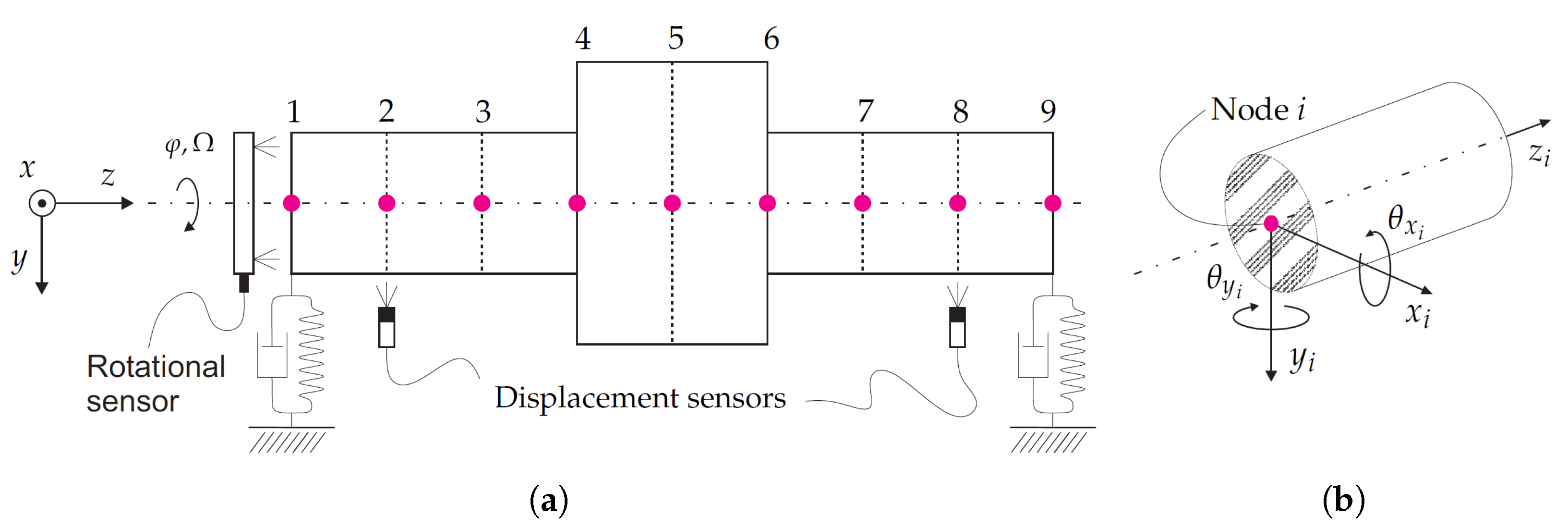
2.1. Modeling of Rotating Shaft

In this section, a rotating shaft is modeled as an elastic beam. As visualized in Figure 1a, the shaft is assumed to rotate around the z-axis. The mass of the shaft is considered to be unbalanced, so that the resulting unbalance force leads to radial displacement of the beam in x and y-directions. Based on finite element method [18], the dynamics of displacements of the shaft can be modeled as
M d ¨ + D d ˙ + K d = B ¯ u F u + B ¯ g G ,
where M R 36 × 36 , D R 36 × 36 , K R 36 × 36 describe the mass, damping, and stiffness of the shaft; d R 36 comprises the coordinates of the nodes; F u R 2 with its input matrix B ¯ u R 36 × 2 describes excitation resulting from the unbalance force; and G = m g R with input matrix B ¯ g R 36 describes excitation resulting from gravity, where m R is the mass of the shaft without the unbalance mass. The vector d R 36 is defined as
d = [ y 1 x 1 θ y 1 θ x 1 y 2 x 2 θ y 2 θ x 2 y 9 x 9 θ y 9 θ x 9 ] ,
where θ y i , θ x i R are angles and y i , x i R are displacements around the y and x axis at node i (Figure 1b). The derivation of the matrices M, D, K can be found in Appendix A. The unbalance force and its input matrix are given as
F u = F u y F u x = m u Ω 2 γ sin ( φ ) cos ( φ ) , B ¯ u = 0 16 × 2 1 0 0 1 0 18 × 2 ,
where m u R is the unbalance mass, γ R is the distance between the unbalance mass and the geometric center, and φ R and Ω R are the rotating angle and angular velocity of the shaft. The gravity is distributed over all nodes leading to
B ¯ g = 1 9 1 0 0 0 1 0 0 0 1 0 0 0 .

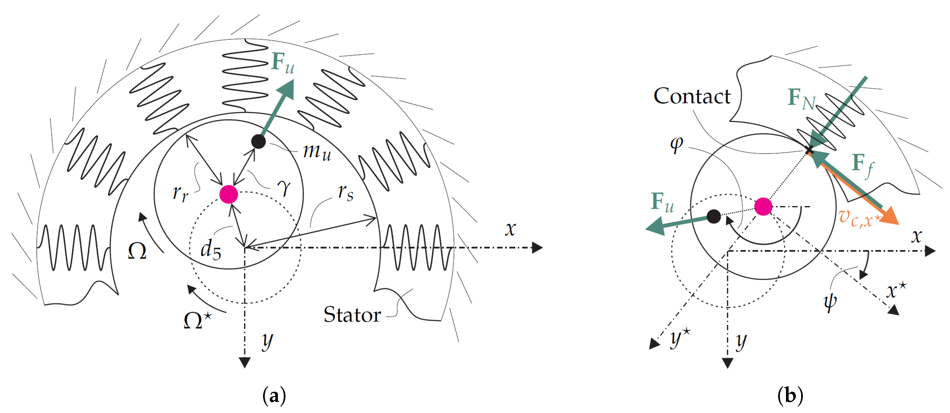
2.2. Modeling of Stator–Rotor Contact

The unbalance force leads to radial displacement of the nodes. If the displacement exceeds the clearance, contact between rotor and stator occurs. It is assumed that the contact occurs at node five.
As visualized in Figure 2a, the distance d c R between the stator and rotor at node five is given by
d c ( y 5 , x 5 ) = d 5 ( y 5 , x 5 ) + r r r s = d 5 ( y 5 , x 5 ) r 0 ,
where r r R is the radius of the rotor, r s R is the inner radius of the stator, r 0 R is the clearance, and d 5 R is the displacement of node five, known as
d 5 ( y 5 , x 5 ) = y 5 2 + x 5 2 .
It follows from (5) that d c 0 characterizes contact and d c < 0 characterizes no contact. In the literature, it is common to model rotor–stator, rotor-bearing, or rotor-casing contact forces by spring and damper elements [5,6,19,20]. In this contribution, the bearing forces are modeled by springs and dampers but without clearance and without rub. The focus is on the contact of rotor and stator with rub. Following [5,6], this contact is modeled by a set of radial springs as visualized in Figure 2. The springs generate the normal force F N = k ¯ d c R , where k ¯ = k s 10 9 > 0 R denotes the constant stiffness of the springs and k s is the prefactor of the spring stiffness. The factor 10 9 results from high values of the Young modulus E Y > 10 9 for the materials in contact. The force of friction is given by the dry friction model F f = μ F N R with friction coefficient μ > 0 R . In addition, lubrication of the contact surfaces can be considered by proper choice of the friction coefficient. The contact force F c R 2 in x y coordinates of the inertial coordinate system is
F c ( y 5 , x 5 , y ˙ 5 , x ˙ 5 , k s , μ ) = F c y F c x = cos ( ψ ) F N sgn ( v c , x ( y 5 , x 5 , y ˙ 5 , x ˙ 5 ) ) sin ( ψ ) F f sin ( ψ ) F N sgn ( v c , x ( y 5 , x 5 , y ˙ 5 , x ˙ 5 ) ) cos ( ψ ) F f , = k s 10 9 d c ( y 5 , x 5 ) d 5 ( y 5 , x 5 ) ( y 5 sgn ( v c , x ( y 5 , x 5 , y ˙ 5 , x ˙ 5 ) ) x 5 μ ) k s 10 9 d c ( y 5 , x 5 ) d 5 ( y 5 , x 5 ) ( x 5 + sgn ( v c , x ( y 5 , x 5 , y ˙ 5 , x ˙ 5 ) ) y 5 μ ) ,
where
v c , x ( y 5 , x 5 , y ˙ 5 , x ˙ 5 ) = x ˙ 5 cos ( ψ ) y ˙ 5 sin ( ψ ) + Ω r r , = 1 d 5 ( y 5 , x 5 ) ( y 5 x ˙ 5 + x 5 y ˙ 5 ) + Ω r r ,
is the velocity of the shaft at the contact point projected on axis x of the body-fixed coordinate system (Figure 2b). The final model that comprises occurance of rotor stator contact is given by
M d ¨ + D d ˙ + K d = B ¯ u F u + B ¯ g G + N ¯ Θ F c ( y 5 , x 5 , y ˙ 5 , x ˙ 5 , k s , μ ) ,
where N ¯ R 36 × 2
N ¯ = 0 1 × 16 1 0 0 1 × 18 0 1 × 16 0 1 0 1 × 18 ,
is the input matrix of the contact force and Θ R is one in the case of contact ( d c 0 ) and zero otherwise ( d c < 0 ). By rearranging (9) and assuming full rank of M, the state-space representation
η ˙ = A η + B u + N Θ ϱ ( η , k s , μ ) ,
with η R 72 , u R 3 , ϱ R 72 , A R 72 × 72 , B R 72 × 3 , and N R 72 × 72 can be achieved. The state vector η is defined as η = d d ˙ , and the input vector u is
u = F u G .
The system matrix A, the input matrix B of known respectively measured inputs, and the input matrix N related to the contact force are
A = 0 36 × 36 I 36 M 1 K M 1 D , B = 0 36 × 2 0 36 × 1 M 1 B ¯ u M 1 B ¯ g , N = I 72 .
Let η ( i ) denote the i-th element of η . The nonlinear term ϱ ( η , k s , μ ) is given by
ϱ ( η , k s , μ ) = 0 36 × 1 M 1 N ¯ F c ( η ( 17 ) , η ( 18 ) , η ( 53 ) , η ( 54 ) , k s , μ ) .
In the following, discretization of the model is discussed. From the well-known discretization rules of linear time-invariant systems (see, e.g., [21]) it follows that the system matrix and input matrix can be discretized as
A d = exp ( A t s ) , B d = A 1 ( A d I 72 ) B ,
where A is assumed to have full rank and t s denotes the sampling time. The contact force related term ϱ ( η , k s , μ ) is assumed to stay constant between two time steps ( k + 1 ) t s and k t s which is a suitable approximation if the sampling time is sufficient small. For the piece-wise constant input ϱ ( η , k s , μ ) the corresponding input matrix N can be discretized as
N d = A 1 ( A d I 72 ) N .
Finally, the nonlinear discrete-time model
η k + 1 = A d η k + B d u k + N d Θ k ϱ ( η k , k s , μ ) ,
is achieved.

3. State and Contact Force Estimation
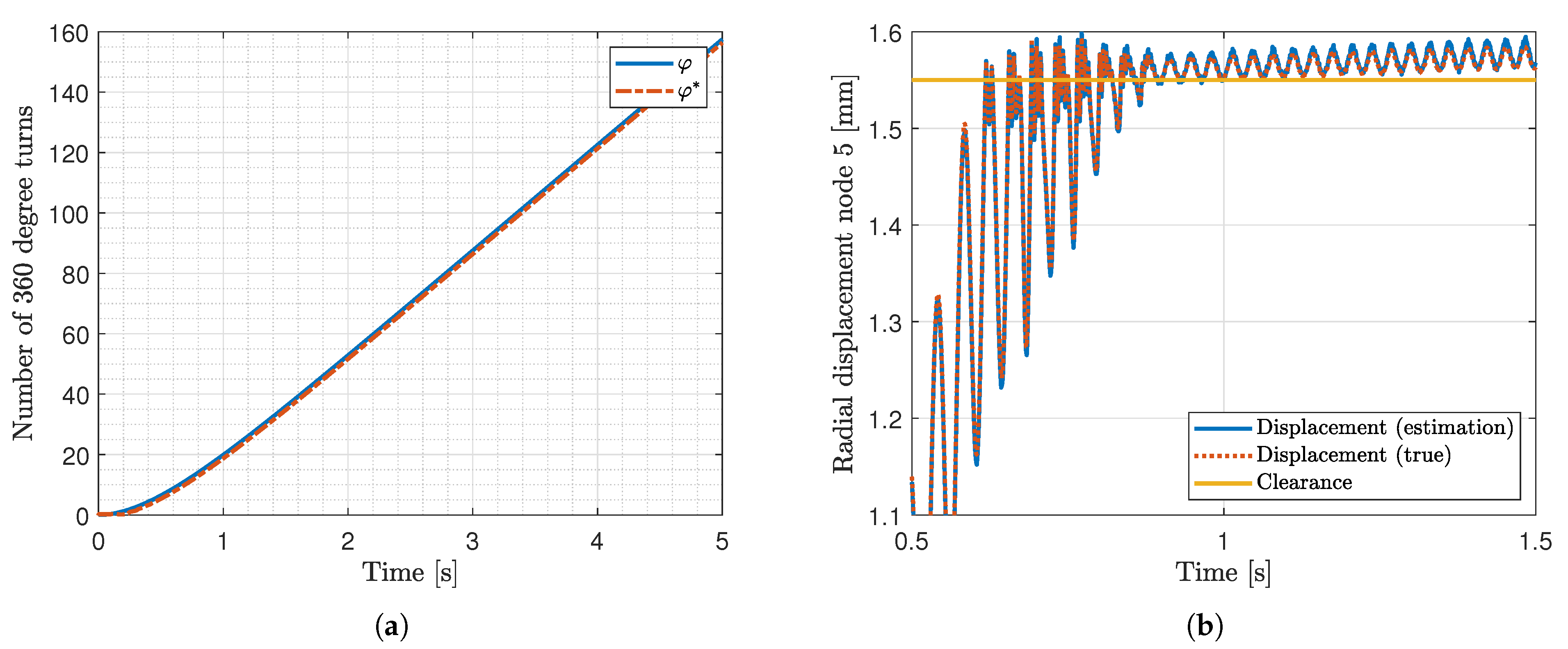
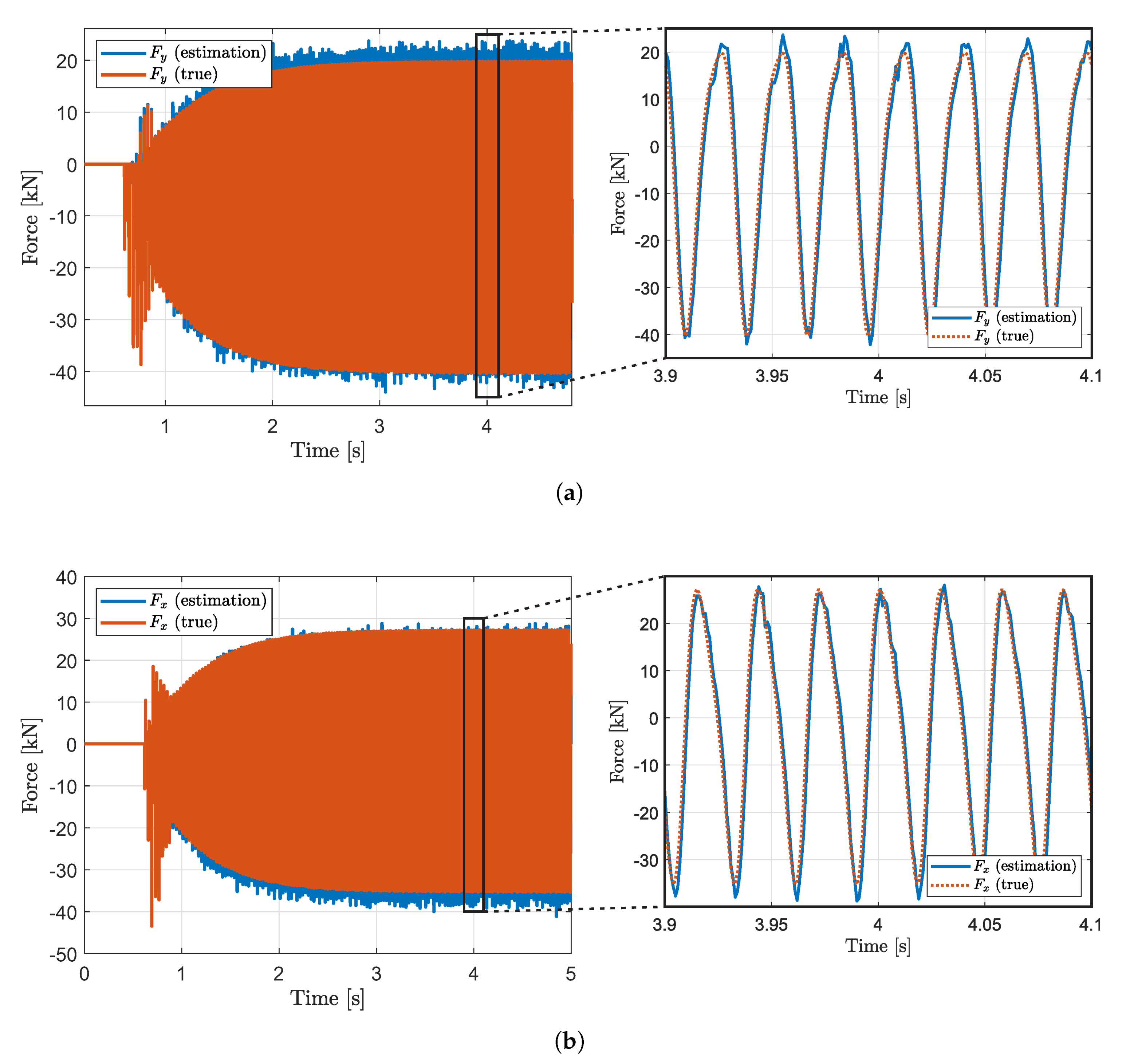
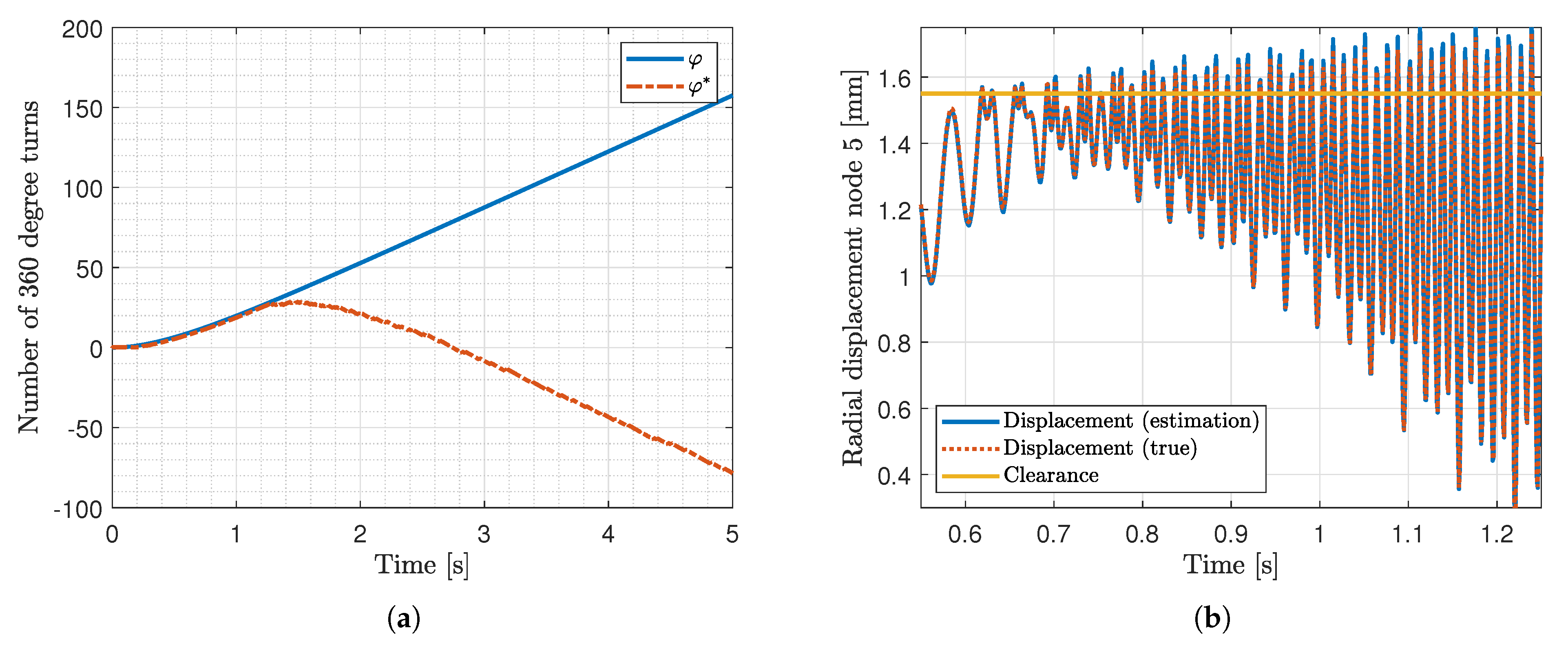
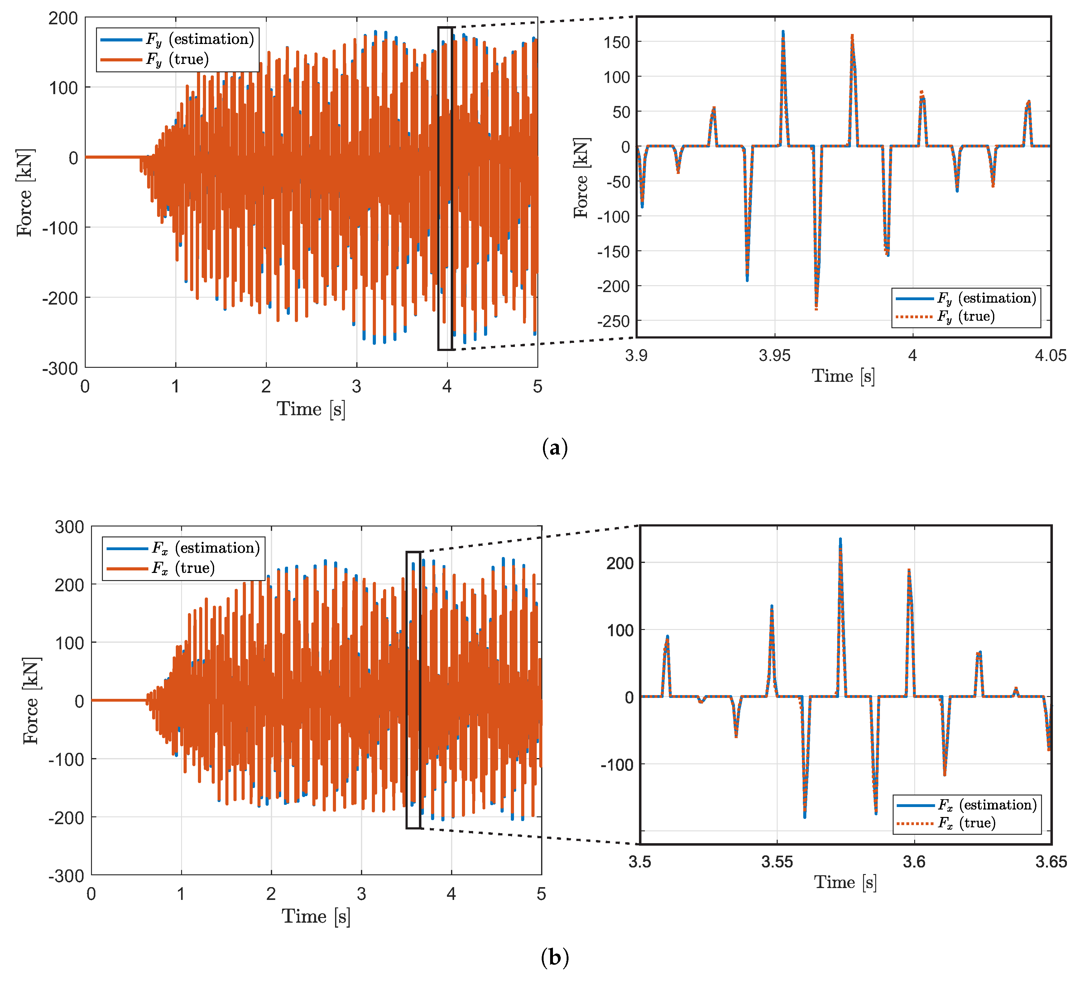
It is assumed that the parameters k s and μ of the introduced model (17) are unknown. The contact force can be estimated by estimating the state η k and the parameters k s and μ of (17). By applying the contact force model (7), the estimations of the contact force are achieved. The parameters k s and μ are estimated based on augmented state Kalman filtering. The discrete-time model (17) is augmented by the dynamics of k s and μ leading to
η k + 1 k s k + 1 μ k + 1 ζ k + 1 = A d η k + B d u k + N d Θ k ϱ ( η k , k s k , μ k ) k s k μ k f ( ζ k , u k , Θ k ) + q η k q s k q μ k q k ,
where ζ k R 74 is the augmented state vector. The parameters k s and μ are indeed constants such that (18) describes the true dynamics. The vector of process noise q k R 74 is introduced to account for discretization and modeling errors. The noise q k is assumed to be zero-mean, white, and to have covariance
Q = E q η k q s k q μ k q η k q s k q μ k = σ η 2 I 72 0 72 × 1 0 72 × 1 0 1 × 72 σ k s 2 0 0 1 × 72 0 σ μ 2 ,
with standard deviations σ η , σ k s , σ μ R and σ η , σ k s , σ μ > 0 . The augmented state model (18) is nonlinear. Consequently, the extended Kalman filter is applied. Therefore, the Jacobian Φ k = f ζ k R 74 × 74 has to be calculated, which is
Φ k ( ζ k , u k , Θ k ) = f ( ζ k , u k , Θ k ) ζ k = A d 0 72 × 1 0 72 × 1 0 1 × 72 1 0 0 1 × 72 0 1 + N d Θ k ϱ ( η k , k s k , μ k ) ζ k 0 1 × 74 0 1 × 74 ,
with ϱ / ζ k R 72 × 74 as
ϱ ζ k = 0 36 × 74 M 1 N ¯ F c ( η k , k s k , μ k ) ζ k ,
and F c / ζ k R 2 × 74 specified as
F c ζ k = Θ k 0 1 × 16 F c y ζ k ( 17 ) F c y ζ k ( 18 ) 0 1 × 54 F c y ζ k ( 73 ) F c y ζ k ( 74 ) 0 1 × 16 F c x ζ k ( 17 ) F c x ζ k ( 18 ) 0 1 × 54 F c x ζ k ( 73 ) F c x ζ k ( 74 ) ,
where
F c y ζ k ( 17 ) = 10 9 ζ k ( 73 ) + r 0 10 9 ζ k ( 18 ) ζ k ( 73 ) ζ k ( 18 ) Γ k ζ k ( 17 ) ζ k ( 74 ) ( ζ k 2 ( 17 ) + ζ k 2 ( 18 ) ) ζ k 2 ( 17 ) + ζ k 2 ( 18 ) ,
F c y ζ k ( 18 ) = 10 9 Γ k ζ k ( 73 ) ζ k ( 74 ) + r 0 10 9 ζ k ( 17 ) ζ k ( 73 ) Γ k ζ k ( 17 ) ζ k ( 74 ) ζ k ( 18 ) ( ζ k 2 ( 17 ) + ζ k 2 ( 18 ) ) ζ k 2 ( 17 ) + ζ k 2 ( 18 ) ,
F c y ζ k ( 73 ) = 10 9 ζ k ( 17 ) 10 9 Γ k ζ k ( 18 ) ζ k ( 74 ) + r 0 10 9 ζ k ( 17 ) + Γ k ζ k ( 18 ) ζ k ( 74 ) ζ k 2 ( 17 ) + ζ k 2 ( 18 ) ,
F c y ζ k ( 74 ) = 10 9 Γ k ζ k ( 18 ) ζ k ( 73 ) + r 0 10 9 Γ k ζ k ( 18 ) ζ k ( 73 ) ζ k 2 ( 17 ) + ζ k 2 ( 18 ) ,
F c x ζ k ( 17 ) = 10 9 Γ k ζ k ( 73 ) ζ k ( 74 ) r 0 10 9 ζ k ( 18 ) ζ k ( 73 ) Γ k ζ k ( 18 ) ζ k ( 74 ) + ζ k ( 17 ) ( ζ k 2 ( 17 ) + ζ k 2 ( 18 ) ) ζ k 2 ( 17 ) + ζ k 2 ( 18 ) ,
F c x ζ k ( 18 ) = 10 9 ζ k ( 73 ) + r 0 10 9 ζ k ( 17 ) ζ k ( 73 ) ζ k ( 17 ) + Γ k ζ k ( 18 ) ζ k ( 74 ) ( ζ k 2 ( 17 ) + ζ k 2 ( 18 ) ) ζ k 2 ( 17 ) + ζ k 2 ( 18 ) ,
F c x ζ k ( 73 ) = 10 9 ζ k ( 18 ) + 10 9 Γ k ζ k ( 17 ) ζ k ( 74 ) + r 0 10 9 ζ k ( 18 ) Γ k ζ k ( 17 ) ζ k ( 74 ) ζ k 2 ( 17 ) + ζ k 2 ( 18 ) ,
F c x ζ k ( 74 ) = 10 9 Γ k ζ k ( 17 ) ζ k ( 73 ) r 0 10 9 Γ k ζ k ( 17 ) ζ k ( 73 ) ζ k 2 ( 17 ) + ζ k 2 ( 18 ) ,
and Γ k = sgn v c , x ( k t s ) . The switching functions Γ k , Θ k are assumed to be independent of ζ k , i.e., Γ k ζ k = Θ k ζ k = 0 .
As illustrated in Figure 1a, the displacements of nodes two and eight are measured. The corresponding measurement model
y k = C ζ k + r k ,
with
C = 0 1 × 4 1 0 0 1 × 68 0 1 × 4 0 1 0 1 × 68 0 1 × 28 1 0 0 1 × 44 0 1 × 28 0 1 0 1 × 44 ,
describes four measurements y k R 4 , i.e., the displacements of nodes two and eight in x and y directions. The measurement noise r k R 4 is assumed to be white, zero-mean, with covariance
R = r k r k = σ r 2 I 4 ,
and standard deviation σ r > 0 R .
The Kalman filter is applied to estimate the states of the augmented system. Quantities ζ ^ k , d ^ 5 , k , Θ ^ k , F ^ c y , k + 1 , F ^ c x , k + 1 denote the estimation of ζ k , d 5 , k , Θ k , F c y , k + 1 , F c x , k + 1 . First, the estimated displacement
d ^ 5 , k = ( ζ ^ k ( 17 ) ) 2 + ( ζ ^ k ( 18 ) ) 2 ,
of node five is determined. It is checked if the known clearance r 0 is exceeded or not, i.e.,
Θ ^ k = 1 if d ^ 5 , k r 0 0 , 0 otherwise .
The a priori state estimation
ζ ^ k + 1 | k = f ( ζ ^ k , u k , Θ ^ k ) ,
is obtained from the nonlinear augmented model f. The input vector u k is known and equals u from (12) at time step k. The a priori error covariance is determined as
P k + 1 | k = Λ k P k Λ k + Q ,
where Λ k denotes the Jacobian
Λ k = Φ ( ζ ^ k , u k , Θ ^ k ) ,
known from (20). The a posteriori state estimation is calculated as
ζ ^ k + 1 = ζ ^ k + 1 | k + K k + 1 ( y k + 1 C ζ ^ k + 1 | k ) ,
where y k + 1 are the measured node displacements and K k + 1 denotes Kalman filter gain according to
K k + 1 = P k + 1 | k C ( C P k + 1 | k C + R ) 1 .
The a posteriori error covariance is obtained from
P k + 1 = ( I 74 K k + 1 C ) P k + 1 | k ( I 74 K k + 1 C ) + K k + 1 R K k + 1 .
According to (7), the estimation of the contact forces at time step k + 1 is given by
F ^ c y , k + 1 F ^ c x , k + 1 = F c ζ ^ k + 1 ( 17 ) , ζ ^ k + 1 ( 18 ) , ζ ^ k + 1 ( 53 ) , ζ ^ k + 1 ( 54 ) , ζ ^ k + 1 ( 73 ) , ζ ^ k + 1 ( 74 ) .

4. Results

In the following, the lateral behavior of a rotating shaft under the influence of rotor–stator contact forces is simulated. The system parameters used in the simulation are summarized in Table 1.
The behavior of the shaft during forward and backward whirling is considered with the aim to estimate the appearing contact forces. During forward whirling, the angular velocities Ω and Ω of Figure 2a have the same algebraic signs, whereas during backward whirling, Ω and Ω have opposite signs. The lowest eigenfrequency of the shaft is 23.71 [1/s]. The rotational speed Ω of the shaft is increased according to
0.5 Ω ˙ + Ω = 35 × 2 π , Ω ( t 0 ) = 0 .
A simulation duration of 5 [s] is considered. During that time, the shaft runs through its first eigenmode. The resulting resonance peak leads to stator–rotor contacts. Dependent on the values μ , k s of the dry friction model, forward or backward whirling occurs. The simulated measurement noise has standard deviation σ r = 1 × 10 3 [mm] and the sampling time of the filter is chosen as T s = 0.001 [s]. The initial states and error covariance are ζ ^ = 0 74 × 1 , P 0 = I 74 × 0.0001 . The design parameters σ k s , σ μ are chosen as σ k s = 100 , σ μ = 100 .
Selecting μ , k s as μ = 0.2 , k s = 1 establishes a forward whirl as shown in Figure 3. The unknown radial displacement of node five is estimated well by the filter. The exceedance of the clearance can be correctly detected from the estimated displacements. The estimated contact forces are shown in Figure 4. The forward whirl remains stable until the end of the simulation. A strong vibrational effect can be detected. For both x− and y−components of the contact force, shape as well as amplitude of the true and estimated signal closely fit to each other.
Selecting μ , k s as μ = 0.5 , k s = 1 establishes a backward whirl as visualized by Figure 5. It can be seen that the displacement of node five is correctly estimated so that the exceedance of the clearance can be detected. The backward whirl remains stable for the remaining simulation time. In comparison to the forward whirl, more than four times higher amplitude values can be observed, which also vary in time. The estimations of the contact forces are visualized in Figure 6. Again, shape and amplitude of true and estimated signals closely fit to each other.
In the following, the contact force estimation performance is quantified based on the measures
F c x , k 0 : p x , k = | F ^ c x , k F c x , k | | F c x , k | × 100 [ % ] ,
F c y , k 0 : p y , k = | F ^ c y , k F c y , k | | F c y , k | × 100 [ % ] .
For both scenarios, the performance measures are stated in Table 2. The performance measures are sensitive to relatively high estimation errors occuring when | F c x , k | or | F c y , k | are small. However, from Figure 4 and Figure 6, it is known that the amplitudes of the contact forces are large most of the time. For that reason, the performance values (44), (45) are evaluated for all | F c y , k | > 5000 and | F c x , k | > 5000 additionally.

5. Conclusions

In this paper, an estimation strategy suitable to estimated forces resulting from stator–rotor contacts is proposed. An augmented system description is developed that exactly describes the system dynamics for the considered type of contact force. The extended Kalman filter (EKF) is applied to an augmented system description to estimate the system states including contact forces. The signals of the estimated and true contact forces closely fit to each other regarding shape and amplitude. Apart from the EKF, other nonlinear filtering approaches may be applied to the proposed model in the future. In addition, plastic deformation could be considered.

Author Contributions

Conceptualization, M.S. and D.S.; methodology, M.S. and D.S.; software, M.S.; validation, M.S. and D.S.; writing—original draft preparation, M.S.; writing—review and editing, D.S.; supervision, D.S.; project administration, D.S. All authors have read and agreed to the published version of the manuscript.

Funding

We acknowledge support by the Open Access Publication Fund of the University of Duisburg-Essen.

Institutional Review Board Statement

Not applicable.

Informed Consent Statement

Not applicable.

Data Availability Statement

The data presented in this study are available on request from the corresponding author. The data are not publicly available because the data can be easily generated by the reader based on the descriptions of the paper.

Acknowledgments

The authors would like to thank the reviewers for their valueable comments.

Conflicts of Interest

The authors declare no conflict of interest.

Appendix A. Finite Element Modeling

In the following, the lateral displacement of the rotor is described based on the principals of finite-element modeling. The mass-, stiffness-, and damping matrices of the considered beam elements can be found in [18] for instance. The lateral displacement of the rotor shown in Figure 1a is described by the following model
M 0 d ¨ 0 + D 0 d ˙ 0 + K 0 d 0 = B ¯ u F u + B ¯ g G ,
where the forces resulting from the bearings are not yet considered. The eight beam elements form the mass M 0 R 36 × 36 , stiffness K 0 R 36 × 36 , and damping matrices D 0 R 36 × 36 according to
M 0 = T A M ¯ T A , K 0 = T A K ¯ T A , D 0 = α K 0 + β M 0 ,
with M ¯ , K ¯ R 64 × 64 specified as
M ¯ = M i 0 0 0 M i 0 0 0 M i , K ¯ = K i 0 0 0 K i 0 0 0 K i ,
and M i , K i R 8 × 8 given as
M i = ρ Σ i l i 420 156 0 0 22 l i 54 0 0 13 l i 0 156 22 l i 0 0 54 13 l i 0 0 22 l i 4 l i 2 0 0 13 l i 3 l i 2 0 22 l i 0 0 4 l i 2 13 l i 0 0 3 l i 2 54 0 0 13 l i 156 0 0 22 l i 0 54 13 l i 0 0 156 22 l i 0 0 13 l i 3 l i 2 0 0 22 l i 4 l i 2 0 13 l i 0 0 3 l i 2 22 l i 0 0 4 l i 2 ,
K i = E Y J i l i 3 12 0 0 6 l i 12 0 0 6 l i 0 12 6 l i 0 0 12 6 l i 0 0 6 l i 4 l i 2 0 0 6 l i 2 l i 2 0 6 l i 0 0 4 l i 2 6 l i 0 0 2 l i 2 12 0 0 6 l i 12 0 0 6 l i 0 12 6 l i 0 0 12 6 l i 0 0 6 l i 2 l i 2 0 0 6 l i 4 l i 2 0 6 l i 0 0 2 l i 2 6 l i 0 0 4 l i 2 .
The quantities used are: the material density ρ R , the cross section of the i-th beam element Σ i R , the length of the i-th beam element l i R , the Young modulus E Y R , the second moment of area of the i-th beam element J i R , and the damping factors α , β R . The transformation matrix T A R 64 × 36 describes the relation
v = T A d ,
between the generalized coordinates of the eight beam elements v R 64
v = [ y 1 l x 1 l θ y 1 l θ x 1 l y 1 r x 1 r θ y 1 r θ x 1 r y 2 l x 2 l θ y 2 l θ x 2 l y 2 r x 2 r θ y 2 r θ x 2 r y 8 l x 8 l θ y 8 l θ x 8 l y 8 r x 8 r θ y 8 r θ x 8 r ] T ,
and the displacements and bending angles of the nine nodes d R 36 are known from (2).
In the following, the presently missing forces resulting from the bearings are considered. The excitation p b R 36 of system (A1) resulting from the bearings can be described by
p b = k b Π d d b Π d ˙ ,
with spring stiffness k b R and damper coefficient d b R . The location of the forces are defined by Π R 36 × 36
Π = 1 0 0 0 0 1 0 0 0 30 × 1 0 30 × 1 0 30 × 1 0 30 × 1 0 0 1 0 0 0 0 1 0 2 × 1 0 2 × 1 0 2 × 1 0 2 × 1 1 0 0 1 × 30 0 0 0 0 0 1 0 1 × 30 0 0 0 0 0 0 0 1 × 30 1 0 0 0 0 0 0 1 × 30 0 1 0 0 .
Considering p b to affect system (A1), it follows that
M 0 d ¨ + D 0 d ˙ + K 0 d = B ¯ u F u + B ¯ g G k b Π d d b Π d ˙ .
Consequently, the matrices of model (1) are achieved as
M = M 0 , D = D 0 + d b Π , K = K 0 + k b Π .

References

  1. Jacquet-Richardet, G.; Torkhani, M.; Cartraud, P.; Thouverez, F.; Baranger, T.N.; Herran, M.; Gibert, C.; Baguet, S.; Almeida, P.; Peletan, L. Rotor to stator contacts in turbomachines. Review and application. Mech. Syst. Signal Process. 2013, 40, 401–420. [Google Scholar] [CrossRef] [Green Version]
  2. Ma, H.; Zhao, Q.; Zhao, X.; Han, Q.; Wen, B. Dynamic characteristics analysis of a rotor–stator system under different rubbing forms. Appl. Math. Model. 2015, 39, 2392–2408. [Google Scholar] [CrossRef]
  3. Chamroon, C.; Cole, M.O.; Wongratanaphisan, T. An active vibration control strategy to prevent nonlinearly coupled rotor–stator whirl responses in multimode rotor-dynamic systems. IEEE Trans. Control Syst. Technol. 2013, 22, 1122–1129. [Google Scholar] [CrossRef] [Green Version]
  4. Jiang, J.; Shang, Z.; Hong, L. Characteristics of dry friction backward whirl—A self-excited oscillation in rotor-to-stator contact systems. Sci. China Technol. Sci. 2010, 53, 674–683. [Google Scholar] [CrossRef]
  5. Jiang, J. Determination of the global responses characteristics of a piecewise smooth dynamical system with contact. Nonlinear Dyn. 2009, 57, 351–361. [Google Scholar] [CrossRef] [Green Version]
  6. Varney, P.; Green, I. Nonlinear phenomena, bifurcations, and routes to chaos in an asymmetrically supported rotor–stator contact system. J. Sound Vib. 2015, 336, 207–226. [Google Scholar] [CrossRef]
  7. Prabith, K.; Krishna, I.P. The numerical modeling of rotor–stator rubbing in rotating machinery: A comprehensive review. Nonlinear Dyn. 2020, 101, 1317–1363. [Google Scholar] [CrossRef]
  8. Ehehalt, U.; Alber, O.; Markert, R.; Wegener, G. Experimental observations on rotor-to-stator contact. J. Sound Vib. 2019, 446, 453–467. [Google Scholar] [CrossRef]
  9. Chipato, E.T.; Shaw, A.D.; Friswell, M.I. Nonlinear rotordynamics of a MDOF rotor–stator contact system subjected to frictional and gravitational effects. Mech. Syst. Signal Process. 2021, 159, 107776. [Google Scholar] [CrossRef]
  10. von Groll, G.T.; Ewins, D.J. A mechanism of low subharmonic response in rotor/stator contact—Measurements and simulations. J. Vib. Acoust. 2002, 124, 350–358. [Google Scholar] [CrossRef]
  11. Varney, P.; Green, I. Rotordynamic analysis of rotor–stator rub using rough surface contact. J. Vib. Acoust. 2016, 138. [Google Scholar] [CrossRef]
  12. Kuseyri, İ.S. Robust control and unbalance compensation of rotor/active magnetic bearing systems. J. Vib. Control 2012, 18, 817–832. [Google Scholar] [CrossRef]
  13. Kitanidis, P.K. Unbiased minimum-variance linear state estimation. Automatica 1987, 23, 775–778. [Google Scholar] [CrossRef]
  14. Gillijns, S.; De Moor, B. Unbiased minimum-variance input and state estimation for linear discrete-time systems. Automatica 2007, 43, 111–116. [Google Scholar] [CrossRef]
  15. Friedland, B. Treatment of bias in recursive filtering. IEEE Trans. Autom. Control 1969, 14, 359–367. [Google Scholar] [CrossRef]
  16. Hmida, F.B.; Khémiri, K.; Ragot, J.; Gossa, M. Three-stage Kalman filter for state and fault estimation of linear stochastic systems with unknown inputs. J. Frankl. Inst. 2012, 349, 2369–2388. [Google Scholar] [CrossRef]
  17. Ding, B.; Zhang, T.; Fang, H. On the equivalence between the unbiased minimum-variance estimation and the infinity augmented kalman filter. Int. J. Control 2020, 93, 2995–3002. [Google Scholar] [CrossRef]
  18. Klein, B. Grundlagen und Anwendungen der Finite-Element-Methode im Maschinen-und Fahrzeugbau; Springer Vieweg: Wiesbaden, Germany, 2012. [Google Scholar]
  19. Yu, J.; Goldman, P.; Bently, D.; Muzynska, A. Rotor/seal experimental and analytical study on full annular rub. J. Eng. Gas Turbines Power 2002, 124, 340–350. [Google Scholar] [CrossRef]
  20. Kim, Y.B.; Noah, S. Quasi-periodic response and stability analysis for a non-linear Jeffcott rotor. J. Sound Vib. 1996, 190, 239–253. [Google Scholar] [CrossRef]
  21. Kwakernaak, H.; Sivan, R. Linear Optimal Control Systems; John Wiley & Sons: Hoboken, NJ, USA, 1972; Volume 1. [Google Scholar]
Figure 1. Finite element modeling of elastic rotor. (a) Shaft rotating around the z axis with angle φ and angular velocity Ω . Rotating shaft modeled by eight elastic beam elements with nine nodes. Displacements of node two and eight in x and y directions and rotating angle φ measured. (b) Each node i is described by displacements x i , y i and angles θ x i , θ y i .
Automation 02 00005 g001
Figure 2. Radial displacement and stator–rotor contact. (a) Radial displacement d 5 of node five and rotation of node five around z axis with angular velocity Ω . Both effects are caused by unbalanced mass m u , which generates unbalance force F u . (b) Rotor–stator contact with normal force F s and force of friction F f . Body-fixed coordinate system with axis x , y rotating with shaft. Velocity v c , x is velocity of rotating shaft at contact point projected on the x axis.
Automation 02 00005 g002
Figure 3. Visualization of forward whirl. (a) Rotating angles φ ( t ) = t 0 t Ω d τ and φ ( t ) = t 0 t Ω d τ with Ω , Ω defined by Figure 2a. (b) Time span in which radial displacement exceeds clearance for the first time. Visualization of true and estimated radial displacements.
Automation 02 00005 g003
Figure 4. Visualization of true and estimated contact forces during forward whirl. Components x and y with respect to inertial coordinate system. (a) y−component. (b) x−component.
Automation 02 00005 g004
Figure 5. Visualization of backward whirl. (a) Rotating angles φ ( t ) = t 0 t Ω d τ and φ ( t ) = t 0 t Ω d τ with Ω , Ω defined by Figure 2a. (b) Time span in which radial displacement exceeds clearance for the first time. Visualization of true and estimated radial displacements.
Automation 02 00005 g005
Figure 6. Visualization of true and estimated contact forces during backward whirl. Components x and y with respect to inertial coordinate system. (a) y−component. (b) x−component.
Automation 02 00005 g006
Table 1. Parameters of lateral rotor vibration model.
DescriptionParameterUnitValue
Length of beam elements l i with i A m437.5
Cross section area Σ i with i B mm 2 159,043
Σ j with j C mm 2 31,416
Material density ρ kg / m 3 7850
Shaft massmkg863
Unbalance mass m u kg20
Displacement of unbalance mass γ mm35
Young modulusE kg / mms 2 190 × 10 4
Second moment of area J i with i B mm 4 2.01 × 10 9
J j with j C mm 4 7.85 × 10 7
Spring coefficient (bearing) k b N / m 10 × 10 8
Damper coefficient (bearing) d b Ns / m 1000
Damping coefficients (shaft) α -0.002
β -0.002
Clearance r 0 mm1.55
Sets of beam elements: A = { 1 ,   2 ,   3 ,   4 ,   5 ,   6 ,   7 ,   8 } ,   B = { 4 ,   5 } ,   C = { 1 ,   2 ,   3 ,   6 ,   7 ,   8 } .
Table 2. Quantification of contact force estimation performance.
Mean p x , k Mean p y , k Median p x , k Median p y , k
Forward whirl219.54257.3421.0321.01
Backward whirl78.8980.5115.8916.36
Forward whirl *24.3024.2116.9017.09
Backward whirl *22.4423.0512.2613.06
* Only larger quantities i.e., F c y , k :   | F c y , k | > 5000 and F c x , k :   | F c x , k | > 5000 .
Publisher’s Note: MDPI stays neutral with regard to jurisdictional claims in published maps and institutional affiliations.

