
Article

Deadline-Aware Scheduler-Weight Adaptation for 5G NR V2X Networks Using Probabilistic Prediction and Reinforcement Learning


by
Gerasimos Papanikolaou-Ntais
1,*,
Dionysios N. Sotiropoulos
1,
Athanasios Kanavos
2 and
Alexandros Kaloxylos
2
1
Department of Informatics, University of Piraeus, 80 Karaoli & Dimitriou Str., 185 34 Piraeus, Greece
2
Department of Informatics and Telecommunications, University of Peloponnese, 221 31 Tripoli, Greece
*
Author to whom correspondence should be addressed.
Telecom 2026, 7(4), 80; https://doi.org/10.3390/telecom7040080
Submission received: 27 May 2026 / Revised: 18 June 2026 / Accepted: 23 June 2026 / Published: 1 July 2026

Abstract

5G New Radio Vehicle-to-Everything (NR V2X) networks must support heterogeneous traffic with strict and diverse latency requirements. Conventional proportional-fair (PF) scheduling does not explicitly account for packet deadlines, which can lead to deadline violations for critical vehicular services under congestion. This paper studies deadline-aware MAC scheduler-weight adaptation for 5G NR V2X using probabilistic prediction and reinforcement learning. We implement a closed-loop ns-3/5G-LENA framework in which network telemetry is exchanged with a Python control agent through ns3-ai shared memory. Gaussian Mixture Model (GMM), Hidden Markov Model (HMM), and Bayesian Logistic Regression (BLR) classifiers are used to predict imminent deadline violations. Their outputs are either mapped directly to scheduler weights or provided as additional state information to a Proximal Policy Optimization (PPO) agent. We evaluate ten scheduling strategies: PF, a non-learning Slack-Based Deadline-Aware Scheduler (SB-DAS), three classifier-only controllers, three classifier-assisted PPO variants, PPO-only, and PPO-only with safety shielding. Experiments are conducted across three vehicle densities and three random seeds per density, using the Deadline-Constrained Packet Reception Ratio (DC-PRR) as the main metric. The PF baseline achieves 61.55% mean DC-PRR and degrades from 75.2% at 30 vehicles to 44.1% at 60 vehicles. In contrast, all adaptive strategies exceed 95% mean DC-PRR and recover 34–38 percentage points over PF in every paired density/seed comparison. The main result is therefore the robust gap between PF and deadline-aware adaptation. Differences among the adaptive controllers are much smaller and fall within the observed seed-to-seed variability. In particular, SB-DAS, which uses no classifier, neural network, or training, achieves DC-PRR statistically indistinguishable from the learned and probabilistic controllers. This indicates that, in the evaluated scenarios, most of the gain comes from deadline awareness itself rather than from learning. We also find that adding classifier-derived violation probabilities to PPO does not consistently improve performance over PPO using raw telemetry alone. To support reproducibility and deployment assessment, the paper includes detailed parameter tables, reward-coefficient and sensitivity analysis, scheduler-weight sensitivity, and per-controller inference-latency and complexity measurements.

1. Introduction

1.1. Motivation

New Radio Vehicle-to-Everything (NR V2X) extends LTE V2X from periodic awareness messaging toward advanced cooperative driving services with stricter and more diverse communication requirements. While LTE V2X mainly supported the broadcast of messages such as Cooperative Awareness Messages (CAMs) and Decentralized Environmental Notification Messages (DENMs), NR V2X targets demanding and safety-critical use cases such as teleoperated driving, cooperative perception, automated intersection control, road-traffic safety applications, and high-definition map distribution [1,2]. These services differ significantly in packet size, traffic periodicity, direction, criticality, and latency budget.
This heterogeneity creates a difficult scheduling problem at the gNB. In a dense urban scenario, safety-critical flows may coexist with high-throughput but delay-tolerant services. Teleoperated driving or automated intersection control may require packets to be delivered within a few tens of milliseconds, while HD map updates can usually tolerate larger delays but consume a significant share of the available bandwidth. When the cell becomes congested or the channel quality fades, the scheduler must decide not only which UE has favorable channel conditions, but also which packets are close to becoming unusable because their deadline is about to expire.
This distinction is important because a packet that arrives beyond its deadline has no value for safety-critical applications, even if it is eventually received. A teleoperation command delivered after its control deadline, or a safety-awareness packet delivered too late to support a driving decision, should not be counted as a successful service outcome. In addition, these deadline violations introduce safety hazards for the road users. A teleoperated vehicle flow receiving packets with delay might also delay the actual steering and control of the vehicle. For this reason, we adopt the Deadline-Constrained Packet Reception Ratio (DC-PRR) as the primary evaluation metric. DC-PRR counts a packet as successful only when it is both received and delivered within its use-case-specific latency deadline.
The problem is further complicated by the dynamics of vehicular radio environments. Vehicle mobility, non-line-of-sight conditions, fading, and changing interference patterns can cause rapid variations in channel quality. A UE with acceptable latency in one control interval may experience degraded conditions in the next, increasing buffer occupancy and reducing the probability that queued packets will meet their deadlines. Static priority assignments are not sufficient in this setting: they may over-prioritize critical traffic under light load, under-prioritize it during congestion, or fail to react to short-lived channel and buffer changes. These observations motivate a scheduler-control mechanism that is both deadline-aware and adaptive.

1.2. Problem Statement

The standard 5G NR MAC scheduler allocates radio resources by evaluating a scheduling metric for each UE and serving UEs according to their metric values. Proportional fair (PF) scheduling, for example, balances instantaneous achievable rate against time-averaged throughput [3]. QoS-aware TDMA schedulers, such as those in the CTTC 5G-LENA ns-3 module [4], extend this principle by allowing per-UE weights to influence the scheduling decision. Although such schedulers are effective for balancing spectral efficiency and fairness, they do not directly optimize deadline satisfaction. Under congestion, naturally, latency increases, and the most delay-sensitive flows are the first to experience deadline violations.
A static-priority solution is also limited. Permanently assigning high weights to critical flows can protect them during congestion but may unnecessarily reduce the throughput of background traffic when the network is lightly loaded. Additionally, a fixed weight ratio may still be insufficient when a critical UE experiences temporary channel degradation or buffer build-up. The scheduling problem therefore requires dynamic weight adaptation based on the current state of each flow, including channel quality, buffer pressure, and remaining deadline budget.
The problem addressed in this paper is the following: given periodic network telemetry from a 5G NR V2X simulation, can a controller predict imminent packet deadline violations and use these predictions to adapt MAC scheduler weights in a way that improves DC-PRR for critical traffic without excessive degradation of background-flow performance, and how do alternative predictor and controller designs compare on this task?

1.3. Proposed Approach and Scope

We propose a closed-loop deadline-aware scheduling framework for 5G NR V2X networks. The framework operates at a 100 ms control period. During each control cycle, ns-3 exports network telemetry to a Python-based control agent through the ns3-ai shared-memory interface. The agent estimates the risk of deadline violation for each UE or flow and returns scheduler-weight actions to the NR QoS-aware TDMA scheduler.
Three probabilistic classifiers are evaluated as deadline-violation predictors: Gaussian Mixture Model (GMM), Hidden Markov Model (HMM), and Bayesian Logistic Regression (BLR). Each model is trained offline using telemetry generated from baseline simulations and predicts whether a deadline violation is likely to occur in the next control window. The resulting violation probability is used in two ways. In the classifier-only variants, it is mapped directly to scheduler-weight levels through threshold-based rules with hysteresis. In the reinforcement-learning variants, it is included as part of the state observed by a Proximal Policy Optimization (PPO) agent.
This work is positioned as a comparative analysis of deadline-aware adaptive scheduling rather than a search for a single optimal controller. The objective is to characterize the design space spanned by lightweight rule-based controllers, learned policies, and hybrids of the two and to quantify their behavior relative to a fairness-oriented baseline. As shown in Section 6, all evaluated AI-assisted variants approach a deadline-satisfaction ceiling under the simulated load range. The dominant finding is therefore the gap between adaptive and non-adaptive scheduling rather than fine-grained ranking among the adaptive methods.
To make this comparison interpretable, the evaluated design space is structured as a PF → heuristic → learned ladder. Beyond the fairness-oriented PF baseline, we include a deterministic, non-learning deadline-aware heuristic, the Slack-Based Deadline-Aware Scheduler (SB-DAS), that maps minimum packet slack and a recent violation ratio onto the same scheduler-weight set as the learned controllers. This intermediate rung makes it possible to attribute the observed gains either to deadline awareness as such or to learning on top of it. As the results show, most of the recovery over PF is already captured by the non-learning heuristic, and the learned controllers do not provide a statistically resolvable gain beyond it under the evaluated conditions.

1.4. Contributions

This paper makes the following contributions:
  • A closed-loop ns-3/ns3-ai framework for AI-assisted scheduler-weight control in 5G NR V2X networks, designed to be modular with respect to the underlying NR MAC scheduler.
  • A formulation of deadline-violation prediction as a binary next-window supervised classification task using rolling-window telemetry, together with the training of three probabilistic classifiers (GMM, HMM, BLR) for this task.
  • A reinforcement-learning controller based on PPO with a deadline-aware reward function, evaluated both standalone and with classifier-derived violation probabilities included as state features.
  • An evaluation of ten scheduling strategies: the PF baseline, the non-learning SB-DAS heuristic, three classifier-only controllers, three classifier-assisted PPO variants, PPO-only, and PPO-only with safety shield, using DC-PRR and supporting metrics across multiple vehicle densities and random seeds.
  • An empirical assessment of whether classifier-derived violation probabilities improve PPO-based scheduler control. Our results suggest that, under the evaluated conditions, the hybrid combination does not provide a consistent benefit beyond standalone classifier or standalone PPO control.
  • A non-learning deadline-aware baseline, the Slack-Based Deadline-Aware Scheduler (SB-DAS), which maps minimum packet slack and a recent violation ratio onto the same scheduler-weight set { 1 , 2 , 5 , 10 } as the proposed controllers. Including SB-DAS enables a fair PF → heuristic → learned comparison and isolates the contribution of deadline awareness from that of learning.
  • Full reproducibility material (software version, hyperparameters, algorithms, reward coefficients, normalization, seeds, and a consolidated notation/parameter table), together with a reward-contribution and coefficient-sensitivity analysis, a scheduler-weight-set rationale and sensitivity analysis, and a per-controller inference-latency and computational-complexity analysis that grounds the deployment-simplicity discussion.

1.5. Paper Organization

Section 2 reviews related work. Section 3 describes the simulated 5G NR V2X environment. Section 4 presents the proposed prediction and scheduler-control framework. Section 5 outlines the experimental methodology, including dataset generation, classifier and PPO training, and the training/evaluation split used for generalization testing. Section 6 reports simulation results. Section 7 discusses findings, limitations, and practical implications. Section 8 concludes the paper with a summary of the results and contributions.

2. Related Work

This section reviews four bodies of literature that intersect with the present work: reinforcement learning for V2X resource allocation (Section 2.1), QoS prediction and violation forecasting in wireless networks (Section 2.2), deadline-aware scheduling in 5G NR (Section 2.3), and safe reinforcement learning with shielding mechanisms (Section 2.4). For each area, we identify the specific gap that our approach addresses.

2.1. Reinforcement Learning Based Resource Allocation for V2X

Deep reinforcement learning (DRL) has been demonstrated as a practical tool for resource allocation in vehicular networks, although the majority of works target the decentralized sidelink rather than centralized gNB MAC scheduling. Liang et al. [5] modeled V2X spectrum sharing as a multi-agent reinforcement learning problem, using a fingerprint-based deep Q-network to assist Vehicle-to-Vehicle (V2V) links in autonomously learning distributed spectrum and power allocation while improving Vehicle-to-Infrastructure (V2I) sum capacity. Ye et al. [6] applied deep RL to V2V resource allocation, optimizing sub-band selection and power control under latency constraints. Shao et al. [7] proposed a semantic-aware resource allocation framework for 5G-V2X heterogeneous networks using PPO, jointly optimizing flexible duty-cycle coexistence and base-station assignment in NR unlicensed bands. Jabeen [8] developed a multi-agent DRL scheduler for IoT–5G-NR coexistence, comparing policy gradient, DQN, and DDPG algorithms for in-band resource block allocation under inter-cell interference.
In centralized scheduling, AL-Tam et al. [9] proposed LEASCH, a deep RL framework that learns MAC-layer scheduling policies for the 5G NR downlink. Gu et al. [10] developed a knowledge-assisted deep RL algorithm for 5G scheduler design targeting time-sensitive traffic, combining DDPG with domain knowledge. Sun and Li [11] designed a DRL-based scheduler with contiguous frequency-domain resource allocation, jointly selecting users and allocating resource blocks through a discretized action space.
While these approaches demonstrate the suitability of RL for wireless and V2X scheduling, they share a common limitation: none incorporate explicit deadline awareness or leverage predictive violation information as part of the RL state representation. The sidelink-centric works [5,6,7,8] operate at the UE level with local observations and do not address the cross-service multiplexing challenge faced by a centralized gNB scheduler that must simultaneously serve URLLC teleoperation commands, periodic awareness messages, and high-throughput background flows. The centralized schedulers [9,10,11] optimize throughput, fairness, or general QoS metrics without considering per-packet deadline constraints across heterogeneous use cases. In contrast, our work provides the gNB MAC layer with per-UE granularity, feeding probabilistic deadline-violation predictions from trained classifiers directly into the PPO agent’s state space, and explicitly tests whether such privileged features improve learned scheduling policies.

2.2. QoS Prediction and Violation Forecasting

A growing body of work applies machine learning to predict QoS metrics in vehicular and cellular networks. Barmpounakis et al. [12] proposed PreQoS, an LSTM-based prediction scheme for V2X communications that forecasts uplink/downlink delay and data rate. Palaios et al. [13] provided a comprehensive study of ML methods for vehicular QoS prediction using real measurements, highlighting challenges such as data non-stationarity and feature selection. Koursioumpas et al. [14] introduced DISTINQT, a distributed privacy-aware learning framework for QoS prediction in beyond-5G networks.
In parallel, anomaly and fault detection methods have been applied to wireless network telemetry. Allahdadi and Morla [15] compared GMMs and HMMs for anomaly detection in 802.11 networks, finding that HMMs yielded higher detection accuracy and lower false alarm rates due to their ability to capture temporal dependencies. Their work is the closest methodological parallel to our classifier comparison, though it targets anomaly detection (classifying the current state) rather than violation prediction (forecasting future events).
Despite these advances, three gaps remain. First, existing QoS prediction works forecast continuous metrics (delay, throughput, data rate) rather than predicting binary deadline violation events; a scheduler needs to know whether a specific flow will miss its deadline in the next time window, a fundamentally different prediction target requiring class-conditional modeling with calibrated probabilities. Second, prior predictions inform the application layer or the network operator but are not fed into the MAC scheduler as real-time control inputs. Third, no prior work compares multiple probabilistic classifiers (GMM, HMM, BLR) head-to-head on the same V2X telemetry dataset for next-window violation prediction. Our work addresses these gaps.

2.3. Deadline-Aware Scheduling in 5G NR

Standard 5G NR schedulers rely on static QoS indicators defined by 5QI values in 3GPP TS 23.501 [16]. TDMA-based QoS schedulers assign fixed priority weights, while PF schedulers balance instantaneous channel quality against long-term throughput averages [3]. Although effective for enhanced mobile broadband (eMBB) traffic, these mechanisms lack temporal urgency awareness: a packet approaching its deadline receives the same scheduling priority as one with ample remaining slack. Classical deadline disciplines such as earliest-deadline-first (EDF) [17] and (modified) largest-weighted-delay-first (M-LWDF) [18] make urgency explicit, but they were designed for single-class queues and do not address the cross-service, per-UE, per-direction multiplexing of heterogeneous V2X flows over a shared NR carrier.
Recent efforts have begun to incorporate deadline awareness into scheduling decisions. Hendaoui et al. [19] proposed a dynamic proactive–reactive scheduling strategy for URLLC in 5G, using XGBoost to predict traffic delays and switching between scheduling modes based on current network conditions. Their work demonstrates the value of prediction-informed scheduling but employs a single deterministic classifier without probabilistic output, targets homogeneous URLLC traffic rather than heterogeneous V2X flows, and uses rule-based mode switching rather than a learned policy. Cohen et al. [20] introduced conformal prediction for URLLC scheduling, providing formal reliability guarantees by dynamically adjusting reserved resources. Their approach addresses two traffic classes (URLLC vs. eMBB) with a single deadline threshold, where V2X environments require simultaneous handling of four or more use cases spanning two orders of magnitude in deadline requirements (20 ms to 1000 ms). Robaglia et al. [21] applied deep RL to schedule uplink IoT traffic with strict deadlines, demonstrating that DRL agents could learn to prioritize deadline-critical packets, but they considered a single deadline class in a generic IoT setting without the asymmetric UL/DL requirements or vehicular mobility that characterize V2X. Kanavos et al. [22] proposed an adaptive scheduling approach for V2N communications, showing that scheduler adaptation could improve vehicular service performance under heterogeneous conditions. Relative to these works, we additionally include a deterministic, non-learning deadline-aware heuristic (SB-DAS, Section 4.6) that shares the exact action space of the learned controllers, so that the comparison spans fairness-oriented PF, a rule-based deadline-aware controller, and learned/probabilistic controllers on a common footing.
Our approach differs from the above in three respects. First, we define a deadline-constrained evaluation metric (DC-PRR) that counts a packet as successfully delivered only if it arrives within its use-case-specific deadline. Second, rather than predicting delay or switching between fixed modes, we use probabilistic classifiers to produce per-flow violation probabilities that are consumed by a PPO agent as continuous state features. Third, our system supports four V2X use cases with deadlines ranging from 20 ms to 1000 ms, requiring fine-grained per-UE, per-direction priority decisions across a heterogeneous traffic mix.

2.4. Safe Reinforcement Learning and Shielding

Pure RL agents cannot guarantee safety during exploration, a limitation for V2X applications where deadline violations may have safety consequences. Alshiekh et al. [23] introduced the foundational shielding framework, proving that a correct-by-construction safety supervisor can enforce temporal-logic specifications while allowing the RL agent to optimize performance within the safe set. Carr et al. [24] extended shielding to partially observable settings.
In wireless scheduling, safety during RL training has received limited attention. Most DRL-based schedulers [5,9,10] train in simulation with standard exploration noise and accept that early-training performance may be poor. Our system incorporates a lightweight safety shield that activates during the first 20 control cycles of training (startup protection) and whenever any critical UE’s estimated slack falls below 5 ms (emergency override). When active, the shield overrides the PPO action with a deterministic fallback policy that assigns the highest weight level to critical flows and the lowest to background flows. The agent observes the shielded action and its reward, so policy learning remains aligned with the safety-constrained trajectory. To our knowledge, no prior work on RL-based wireless scheduling has incorporated an explicit safety shield with this form of shielded-action training.

2.5. Summary and Positioning

The distinguishing features of our approach are: (i) probabilistic classifiers trained for deadline-violation prediction with calibrated per-flow violation probabilities; (ii) integration of these probabilities as privileged state features in a PPO-based RL agent that selects per-UE scheduler weights; (iii) a comparative evaluation of three classifier types combined with PPO, plus classifier-only and PPO-only baselines, yielding eight distinct AI-assisted scheduling strategies, together with a non-learning SB-DAS heuristic that shares the same four-level action space, so the comparison spans the full PF → heuristic → learned design space on a common footing; and (iv) evaluation using the deadline-constrained DC-PRR metric across three vehicle densities and four V2X use cases with deadlines spanning 20 ms to 1000 ms.

3. System Model and Simulation Setup

This section describes the simulated 5G NR V2X environment used to generate training data and evaluate the proposed framework. The simulation follows a single-cell urban deployment in which one 5G NR gNB serves a set of vehicular UEs moving over an urban grid road topology.

3.1. Network Topology

The simulated network consists of a single 5G NR gNB deployed in an urban grid scenario. The gNB provides connectivity to vehicular UEs moving along the road grid according to externally generated SUMO mobility traces. All vehicles remain associated with the serving gNB during the simulation, allowing the study to focus on intra-cell radio resource scheduling. The single-gNB choice is dictated by a current limitation of the 5G-LENA NR module in ns-3, which does not yet support handover. Multi-gNB scenarios with handover are therefore outside the scope of this study and are left for future work.
The topology represents a congested urban V2X setting, such as an intersection area or dense road corridor, where multiple vehicles simultaneously generate uplink and downlink traffic with heterogeneous latency and throughput requirements. Let U = { 1 , 2 , , N } denote the set of vehicular UEs, where N varies across simulated load scenarios. Each UE may generate one or more V2X traffic flows depending on the assigned service type and direction.

3.2. 5G NR Radio Configuration

The radio access network is implemented using the 5G NR module in ns-3 (5G-LENA). The gNB operates in the sub-6 GHz band with a carrier frequency of 4 GHz and a system bandwidth of 25 MHz. The physical-layer numerology is two, corresponding to a subcarrier spacing of 60 kHz. The simulation uses the NR TDMA QoS scheduler at the MAC layer, which is extended through dynamic AI-driven scheduler-weight adaptation. Table 1 summarizes the main radio parameters.
The baseline configuration uses the default PF configuration weights for all UEs, making the scheduler behave as a conventional PF scheduler without explicit deadline-risk awareness. In the AI-assisted variants, these weights are updated during the simulation by the external Python controller through the ns3-ai shared-memory interface, through an injection mechanism developed for the experiments.

3.3. V2X Traffic Model

The traffic model includes multiple V2X service classes with different packet sizes, generation intervals, and latency requirements, creating a mixed-criticality scheduling problem in which ultra-low-latency traffic must coexist with throughput-oriented flows. The simulated service classes are Teleoperated Driving (ToD), Automated Intersection Crossing (AIC), Road Traffic Safety Applications (RTSA), and High-Definition Map Collection and Sharing (HDM).
ToD represents the most delay-sensitive traffic class. In the uplink, ToD may carry sensor or vehicle-state information; in the downlink, remote-control commands or assistance information. AIC and RTSA represent safety-related cooperative driving services: less bandwidth-intensive than HD map updates but still requiring timely delivery. HDM traffic is comparatively delay-tolerant but consumes a larger share of radio resources, especially in the downlink, so it acts as a heavy background load competing with critical traffic under congestion.
Table 2 summarizes the configuration.
Each packet is associated with a use-case-specific latency deadline. A packet contributes positively to DC-PRR only if it is successfully received and its one-way latency does not exceed the corresponding deadline, where packets received after their deadline are treated as deadline failures even when they may not necessarily be lost at the radio or transport layer.

3.4. Mobility Model

Vehicle mobility is generated using SUMO over a Manhattan-grid road topology. The Manhattan layout produces repeated intersections, turns, and varying vehicle separations representative of dense urban V2X conditions. Figure 1 illustrates the simulated Manhattan-grid layout. The generated mobility traces are imported into ns-3 and used to update the position of each vehicular UE during the simulation.
The evaluation considers three vehicle-density levels (30, 40, and 60 vehicles) to study scheduler behavior under increasing radio load. For each density, three random seeds are evaluated, accounting for stochastic effects from traffic generation, mobility variation, and radio-channel conditions. Reported results are averaged across seeds while standard deviations and bootstrap confidence intervals are included to quantify robustness and statistical significance of the results.

3.5. MAC Scheduler and Weight Adaptation

The baseline scheduler is the NR TDMA PF scheduler, obtained by assigning equal weights to all UEs and referred to as the PF baseline hereafter. In the PF baseline, no flow receives additional priority based on deadline risk.
The proposed AI-assisted variants modify this behavior by adapting the scheduler weights every 100 ms. The available weight levels are
W = { 1.0 , 2.0 , 5.0 , 10.0 } ,
where 1.0 is normal priority and larger values progressively increase the probability that the corresponding UE will be scheduled earlier or with more resources. The four levels map onto the operational states a deadline-aware controller must distinguish: normal, mild boost, strong boost, and emergency, and the set W = { 1 , 2 , 5 , 10 } was chosen for four reasons. (i) Interpretable priority semantics: The four levels make both the rule-based mapping and the learned policy’s action space human-auditable. (ii) Multiplicative (super-linear) spacing: The gaps widen ( 1 2 5 10 ), so the normal-to-emergency separation ( 10 × ) is much larger than between adjacent low levels ( 2 × ), yielding a sharp response when a flow becomes urgent while keeping low-urgency adjustments gentle, matching the non-linear cost of a deadline miss. (iii) Small, stable action space: A four-action discrete space keeps the PPO policy and critic tractable and exploration well-conditioned. (iv) Identical action space across all methods: PF, SB-DAS, the classifier-only controllers, and the PPO controllers all emit weights from the same set W , so any performance difference is attributable to the policy rather than to a larger or finer action space. An offline sensitivity analysis against the alternative sets { 1 , 2 , 4 , 8 } and { 1 , 3 , 6 , 10 } is reported in Appendix B; { 1 , 2 , 5 , 10 } provides the strongest normal-vs-emergency contrast while retaining four interpretable levels.

4. Proposed Deadline-Aware Scheduler-Weight Adaptation Framework

This section presents the proposed closed-loop framework for deadline-aware scheduler control. The objective is not to replace the NR MAC scheduler but to control its per-UE priority weights using prediction and reinforcement learning. The framework therefore remains compatible with the existing ns-3 NR scheduler implementation while adding an external control loop and the scheduler-weight injection system.

4.1. Closed-Loop Control Architecture

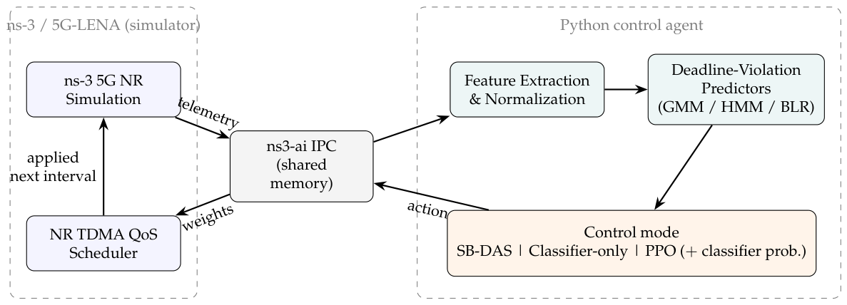
The framework operates as a periodic control loop with discrete phases and actions; Figure 2 depicts the resulting closed loop. Every 100 ms, the ns-3 simulation exports network-state information to an external Python control process through the ns3-ai IPC process. The exported state includes per-flow and per-UE telemetry derived from the current rolling window: latency statistics, packet delivery behavior, buffer pressure, throughput, jitter, and deadline-related indicators. The Python agent computes a scheduling action, either through the heuristic algorithm or through the action from the PPO agent, and sends it back to the simulator, again through the IPC process, before the next control interval.
The framework supports three forms of control. In the SB-DAS configuration, a deterministic slack-and-violation rule maps each flow’s remaining deadline budget directly to a scheduler-weight level, with no trained model (Section 4.6). In the classifier-only configuration, a probabilistic deadline-violation predictor maps violation risk to scheduler weights. In the PPO-based configuration, the violation probability is included in the state observed by a reinforcement learning agent. A PPO-only configuration is also evaluated, where the agent does not receive an explicit classifier output and must rely on the remaining telemetry features. All three forms emit weights from the same four-level set, so they differ only in how the weight level is chosen. The overall closed-loop control procedure is summarized in Algorithm 1.
Algorithm 1 Closed-loop deadline-aware scheduler control
  1: Initialize ns-3 V2X simulation, NR scheduler, and ns3-ai shared-memory interface
  2: Load feature normalizer, trained classifier, and/or trained PPO policy
  3: for each control interval t do
  4:  ns-3 collects telemetry over the current 100 ms window
  5:  Export network state s t through ns3-ai shared memory
  6:  Python controller extracts and normalizes feature vector x t
  7:  if classifier-only mode then
  8:   Estimate violation probability p t = P ( y t + 1 = 1 | x t )
  9:   Map p t to scheduler weight w t using Algorithm 2
10:  else if SB-DAS mode then
11:   Compute minimum slack s t and recent violation ratio v t from telemetry
12:   Map ( s t , v t ) to scheduler weight w t using Algorithm 3
13:  else if PPO mode then
14:   Construct PPO state from telemetry and optional classifier probability p t
15:   Select scheduler-weight action w t using the trained PPO policy
16:   if safety shield is active then
17:    Override w t using the deterministic safety action
18:   end if
19:  end if
20:  Return scheduler weights w t to ns-3 through shared memory
21:  Apply updated weights to the NR TDMA QoS scheduler
22: end for

4.2. Deadline-Violation Prediction Task

The prediction task is formulated as binary next-window classification. At each control time t, the controller observes telemetry from the current 100 ms window and predicts whether the corresponding UE or flow will experience at least one deadline violation during the next control window:
y t + 1 = 1 , if   at   least   one   packet   violates   its   deadline   in   the   next   window , 0 , otherwise .
The formulation is intentionally proactive: the classifier estimates whether a deadline failure is likely to occur shortly after the current observation, so that the scheduler can boost priority before the packet becomes stale. Let x t denote the feature vector extracted from the current control window. Each classifier estimates
p t = P ( y t + 1 = 1 x t ) .

4.3. Feature Extraction

Features are extracted using a rolling 100 ms observation window. For each controlled flow or UE, the 19-dimensional feature vector summarizes recent network behavior and delay pressure: latency statistics (mean, standard deviation, min, max, P75, P90, P95, P99), packet count, bytes received, throughput, mean and minimum slack, observed violation rate, previous-window mean and maximum latency, previous violation rate, latency trend, and the use-case-specific deadline. The rolling-window representation reduces packet-level noise while preserving short-term network dynamics and matches the 100 ms control period.
Features are normalized to a scale of 0 to 1. The same normalization parameters are reused during online inference to avoid distribution mismatch between offline training and live simulation control.

4.4. Probabilistic Classifiers

4.4.1. Gaussian Mixture Model

The Gaussian Mixture Model (GMM) is used as a probabilistic classifier for identifying network states likely to lead to deadline violations in the next control window. V2X telemetry does not follow a single unimodal distribution. Instead, different operating regimes appear in the data (low-latency line-of-sight operation, temporary fading, buffer build-up, congestion). A mixture model represents these regimes through separate Gaussian distributions.
Given a feature vector x t , the GMM scores it under two class-conditional mixtures (violation and non-violation) and converts the resulting class-conditional likelihoods into a posterior through Bayes’ rule. The posterior probability of deadline violation is the classifier output:
p t GMM = π 1 p ( x t y t + 1 = 1 ) c { 0 , 1 } π c p ( x t y t + 1 = c ) , p ( x t y t + 1 = c ) = k = 1 K π c , k N x t μ c , k , Σ c , k ,
where π c is the prior probability of class c { 0 , 1 } , and  π c , k , μ c , k , and  Σ c , k are the weight, mean, and (diagonal) covariance of the k-th of K Gaussian components of the class-c mixture ( K = 5 ; Appendix D).
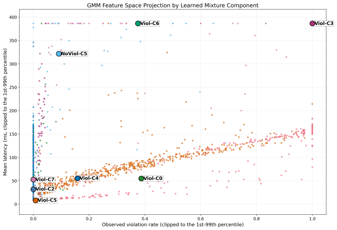
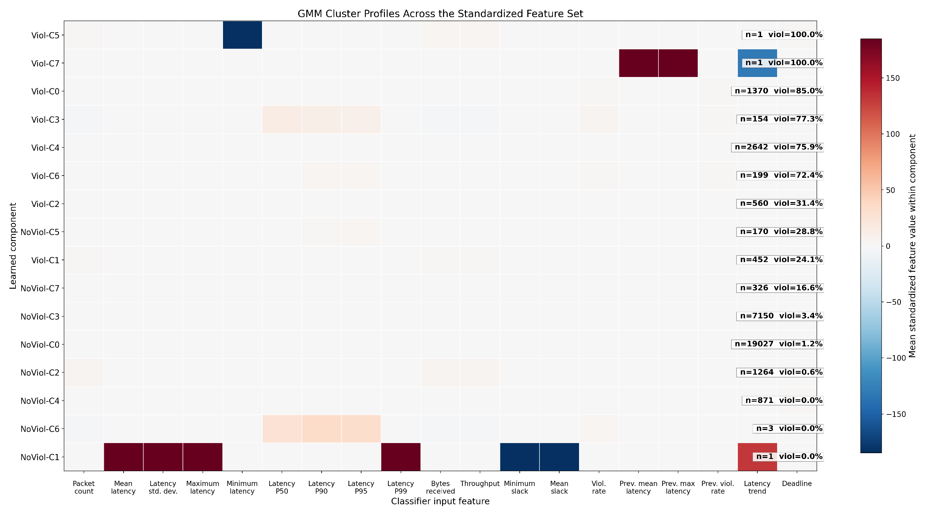
Figure 3 shows the projected GMM feature space, with samples separated according to observed latency and deadline-violation behavior. Components in high-latency or high-violation regions correspond to states where the scheduler should increase priority before packets become stale. Figure 4 provides a feature-level view of the learned components: components associated with higher violation risk exhibit stronger delay, slack, and trend-related signals, indicating that the classifier relies on a multi-feature network-state representation rather than a single latency threshold.

4.4.2. Hidden Markov Model

The Hidden Markov Model (HMM) captures the temporal structure in the telemetry sequence. Unlike the GMM, which treats each observation as a feature-space sample, the HMM models transitions between latent network states. This could prove useful in V2X networks because channel degradation, congestion, and buffer build-up often persist across several control windows. Each observation x t is generated by an unobserved state z t representing a latent radio or traffic regime while the model estimates emission likelihoods and transition probabilities,
P ( z t z t 1 ) , P ( x t z t ) ,
and the predicted violation probability is obtained from the inferred hidden-state distribution:
p t HMM = P ( y t + 1 = 1 x 1 : t ) .
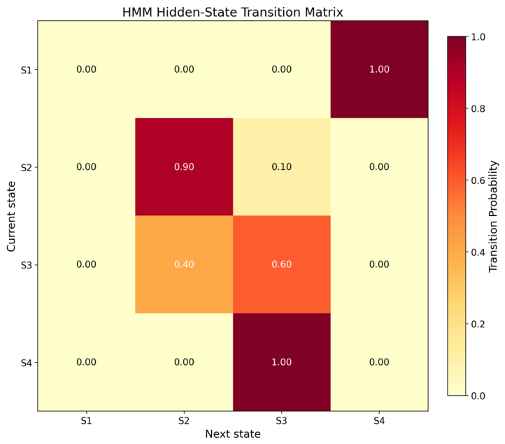
Figure 5 shows the learned transition structure. State S2 corresponds to a persistent healthy regime, S3 to a more persistent congestion or violation-prone regime, and S4 to a transient warning state preceding congestion.

4.4.3. Bayesian Logistic Regression

Bayesian Logistic Regression (BLR) treats logistic-regression parameters as random variables and estimates a posterior distribution over them, allowing the classifier to express uncertainty. For an input feature vector x t ,
p t BLR = P ( y t + 1 = 1 x t , D ) ,
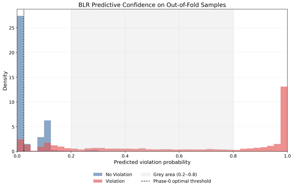
where D is the training dataset. The posterior is approximated using a Laplace approximation. Figure 6 shows that BLR predictions concentrate near 0 and 1 (high-confidence safe and violation-prone samples), with intermediate values reserved for genuinely ambiguous telemetry. This calibration is useful for confidence-aware decision making, although the conservative behavior may reduce recall compared with more aggressive classifiers such as GMM.

4.5. Classifier-Only Scheduler Control

In the classifier-only variants, the predicted violation probability is converted into a scheduler-weight level. Let p t be the classifier output at control time t; the controller applies the threshold rule 
w t = 1.0 , p t < θ 1 , 2.0 , θ 1 p t < θ 2 , 5.0 , θ 2 p t < θ 3 , 10.0 , p t θ 3 .
Lower weights correspond to normal service while higher weights increase scheduling priority for flows at greater risk of missing their deadlines. To avoid oscillations, hysteresis is applied: a weight increase is allowed when the violation probability exceeds the activation threshold, while a decrease requires the probability to fall below a lower deactivation threshold. A collapse-override rule assigns the highest weight if a critical UE has very low estimated slack or a high recent violation ratio, regardless of the classifier threshold (Algorithm 2).
Algorithm 2 Classifier-only probability-to-weight mapping with hysteresis
Require: Violation probability p t , previous weight w t 1 , thresholds θ 1 , θ 2 , θ 3 , hysteresis margin δ
Ensure: Scheduler weight w t
  1: if critical slack is below emergency threshold then
  2:   w t 10.0
  3: else if  p t θ 3  then
  4:   w t 10.0
  5: else if  p t θ 2  then
  6:   w t 5.0
  7: else if  p t θ 1  then
  8:   w t 2.0
  9: else
10:   w t 1.0
11: end if
12: if  w t < w t 1  then
13:  if  w t 1 = 10.0 and p t > θ 3 δ  then
14:    w t w t 1
15:  else if  w t 1 = 5.0 and p t > θ 2 δ  then
16:    w t w t 1
17:  else if  w t 1 = 2.0 and p t > θ 1 δ  then
18:    w t w t 1
19:  end if
20: end if
21: return  w t

4.6. Slack-Based Deadline-Aware Baseline (SB-DAS)

To separate the contribution of deadline awareness from that of learning, we add a deterministic, non-learning controller that runs through the identical NR TDMA-QoS control loop, control period (100 ms), and weight set W = { 1 , 2 , 5 , 10 } as the proposed methods. The Slack-Based Deadline-Aware Scheduler (SB-DAS) uses no classifier, no neural network, and no training: it is a fixed function of telemetry. Each control cycle, for every controlled flow i = ( UE , direction ) it reads the minimum remaining slack s i = D i L i (deadline minus observed latency, in ms) and a recent deadline-violation ratio v i over a five-cycle (500 ms) window and selects a priority level i { 1 , 2 , 3 , 4 } that is mapped to a weight through the same level → weight map as all other controllers (Section 4.7). Background flows (HDM, RTSA) are clamped to level 1. Here, “critical” denotes the tight-deadline ToD and AIC flows, while RTSA and HDM are treated as lower-urgency background flows for the purpose of weight adaptation, owing to their substantially looser latency budgets (Table 2); this controller-level grouping is distinct from the safety relevance of the underlying services. The decision rule is given in Algorithm 3; the slack edges { 50 , 20 , 5 }  ms and the violation threshold 0.2 are listed in the consolidated parameter table (Table A1).
SB-DAS is evaluated at the same three densities (30/40/60 vehicles) and three seeds as every other method, adding nine simulation runs to the evaluation matrix. Because its level decisions are computed directly from slack and the violation ratio rather than from a learned model, SB-DAS is the simplest controller in the comparison and serves as the reference point for the contribution analysis in Section 6.3 and the inference-cost analysis in Section 6.8.
Algorithm 3 SB-DAS slack-to-level mapping with hysteresis (per controlled flow, every 100 ms)
Require: minimum slack s i (ms), recent violation ratio v i , previous level i , edges { 50 , 20 , 5 } , v th = 0.2 , hysteresis margin δ = 5  ms
Ensure: scheduler weight w i
  1:
if flow i is background (HDM/RTSA) then
  2:
i 1
  3:
else if no packet observed in window then
  4:
i 1
▹ normal
  5:
else if  v i > v th  then
  6:
i 4
▹ recent violations
  7:
else if  s i 5  then
  8:
i 4
▹ emergency
  9:
else if  s i 20  then
10:
i 3
▹ strong
11:
else if  s i 50  then
12:
i 2
▹ mild
13:
else
14:
i 1
▹ safe
15:
end if
16:
Hysteresis: upgrades ( i > i ) apply immediately; a downgrade applies only once s i has cleared the previous level’s lower edge by δ ; an emergency/violation always forces i = 4 .
17:
w i { 1 , 2 , 5 , 10 } [ i ]
18:
return  w i

4.7. PPO-Based Scheduler Control

The reinforcement learning agent is based on Proximal Policy Optimization (PPO). PPO was selected because it limits excessive policy updates through a clipped objective, which is useful in a scheduling environment where unstable actions can quickly degrade packet delivery. In addition, the gradual updates of the PPO agent avoid unnecessary oscillations and aggressive, short-lived decisions that might cause extreme actions in the already dynamic V2X environment. The PPO state includes normalized telemetry features (delay statistics, packet delivery behavior, throughput, jitter, buffer pressure, deadline-related indicators), and in the classifier-assisted variants, the state also includes the violation probability produced by GMM, HMM, or BLR. The action space is discrete and identical to the scheduler-weight set W of Equation (1):
A = W = { 1.0 , 2.0 , 5.0 , 10.0 } .

4.7.1. Reward Function

The reward is computed at every control interval. Each served UE i receives a single-currency reward r i = personal i + altruism , where the altruism term is a shared network-health signal and the personal term differs for critical (ToD, AIC) and background (HDM, RTSA) UEs. All coefficients are listed in Table 3.
  • Network health.
Once per cycle, over the set C of critical UEs,
h i = clip s i D i , 0 , 1 slack   score · 1 clip max ( b i ul , b i dl ) b i cap , 0 , 1 1 buffer   pressure , H = 1 | C | i C h i ,
with H = 1 when C = . Here, s i is the minimum remaining slack, D i the use-case deadline, b i ul / dl the buffer occupancy, and  b i cap the buffer capacity.
  • Slack reward.
For a slack value s and deadline D, the bounded, asymmetric slack reward is
R slack ( s , D ) = tanh s / D , s 0 ( [ 0 , + 1 ) ) , 3   tanh s / D , s < 0 ( ( 3 , 0 ] ) .
The deadline D acts as the normalizer (the constant τ s of the schematic form), and the multiplier 3 penalizes a deadline miss far more strongly than equally large positive slack is rewarded.
  • Personal term.
For a critical UE, the personal term sums the uplink and downlink slack rewards and subtracts normalized buffer occupancy,
personal i = R slack ( s i ul , D i ul ) + R slack ( s i dl , D i dl ) b i ul + b i dl .
For a background UE, with weight score g = ( i 1 ) / 3 [ 0 , 1 ] for level i ,
personal i = 4 H g + ( 1 H ) ( 1 g ) 2 ( [ 2 , + 2 ] ) ,
i.e., when the network is healthy, the agent is rewarded for raising background weight (throughput), and when congested for lowering it (altruism).
  • Altruism term and total.
All UEs share
altruism = 2 H 1 ( [ 1 , + 1 ] ) , r i = personal i + altruism .
This makes deadline satisfaction the dominant objective for critical flows while penalizing excessive queueing and the unnecessary starvation of delay-tolerant traffic.

4.7.2. Safety Shield

A lightweight safety shield prevents unsafe actions during early training and emergency conditions. The shield is active during the first 20 control cycles of training (startup protection) and whenever any critical UE’s estimated slack falls below 5 ms. When active, it applies a deterministic fallback: highest priority weight to critical flows, lowest to background flows. The PPO agent observes the shielded action and its reward, so policy learning remains aligned with the safety-constrained trajectory. This approach does not provide formal safety guarantees but reduces catastrophic behavior during exploration. This is an important module in the experiment, since a bad exploratory action by the agent, or even a series of them, might cause a cascading effect in the network that will eventually produce an unrecoverable network state.

5. Experimental Methodology

5.1. Dataset Generation and Train/Evaluation Split

The classifier training dataset was generated from baseline ns-3 simulations using the topology, mobility, and traffic configuration of Section 3. Packet and flow-level telemetry was collected and aggregated into rolling 100 ms windows and each window produced one training sample per controlled UE or flow. For every sample, the feature vector was extracted from the current window and the label from the following window: if at least one packet in the next window violated its use-case-specific deadline, the label was one, otherwise zero. This avoided training the classifiers on data generated by their own interventions and provided a consistent baseline distribution for comparing the probabilistic predictors.

Generalization Split

To test whether the trained controllers generalized beyond their training conditions, we deliberately separated training and evaluation along two axes:
  • Load. PPO policies were trained under stressed conditions: 60-vehicle density with offered packet rates increased by 40% relative to Table 2. Evaluation used the unmodified offered rates and includes 30- and 40-vehicle densities that the agent never saw during training. The 30- and 40-vehicle evaluations therefore constituted a zero-shot generalization test for the learned policies.
  • Mobility. Inference used different SUMO mobility traces (different vehicle trajectories on the same urban grid) and different random seeds from those used for training-data generation. The classifiers and PPO policies were not exposed to the evaluation traces.
Offline processing was used only for dataset construction and classifier training. All reported scheduler-control results were obtained from live ns-3/ns3-ai closed-loop simulations: every controller action was applied to the running simulator and affected subsequent network evolution.

5.2. Classifier Training

The GMM, HMM, and BLR classifiers were trained offline. The dataset was split into training and validation subsets while preserving the temporal ordering of samples where required by the HMM. Feature normalization parameters were computed from the training data and applied consistently during validation and online inference. Classifier performance was evaluated using accuracy, F1-score, precision, recall, ROC-AUC, and average precision. Recall was especially important because a false negative left an at-risk packet without a priority increase; precision mattered because excessive false positives led to unnecessary weight boosts and reduced background-flow throughput. For BLR, probability calibration was additionally evaluated using Expected Calibration Error (ECE).

5.3. PPO Hyperparameter Search

PPO hyperparameters were selected using the Optuna tool. A complete, exhaustive grid search was computationally impractical because each PPO trial required a full ns-3/ns3-ai simulation loop across several hyperparameter selections. The search objective was the DC-PRR score achieved during validation. The search explored learning rate, discount factor, GAE parameter, PPO clipping coefficient, entropy coefficient, and rollout length. Table 4 reports the trials. To keep the search tractable, each Optuna trial used a shortened simulation trace (approximately 8000 s of wall-clock time per trial, as reported in the Elapsed column); only the selected configuration was subsequently trained with the full multi-day budget described in Section 5.4. Trial 9 achieved the highest validation score and was selected as the final configuration: it combined a relatively high learning rate, a short rollout length, and a small clipping coefficient, producing fast adaptation while still constraining policy updates through PPO clipping. The selected trial used an entropy coefficient of 0.020582.

5.4. PPO Training Procedure and Compute Budget

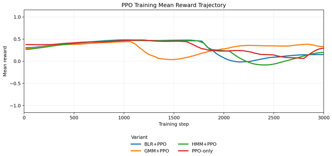
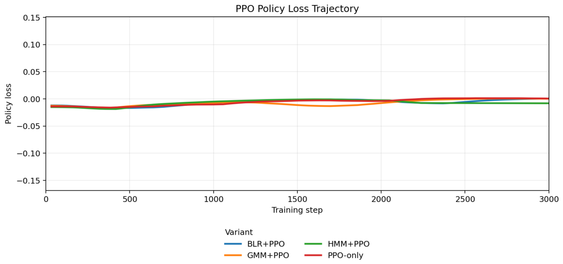
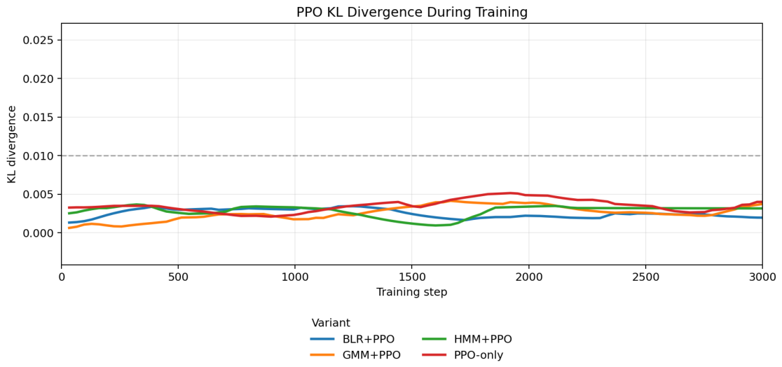
Four PPO variants were trained: PPO-only, GMM+PPO, HMM+PPO, and BLR+PPO. Each PPO training run used a 500 s simulated trace at 60-vehicle density with the +40% traffic stress described above. Because every control step required interaction with the full ns-3/ns3-ai simulation loop, each PPO variant required more than two days of continuous wall-clock training. We therefore evaluated PPO under a fixed, deployment-relevant training budget rather than as an asymptotically converged policy. The training curves in Figure 7, Figure 8 and Figure 9 are reported to show that PPO updates remained bounded and that the learned policies reached a stable operating regime. The final closed-loop inference results in Section 6 are the primary evidence of scheduling effectiveness.

5.5. Compared Scheduling Strategies

We compared ten scheduling strategies:
1.  
PF baseline: PF scheduling with equal weights and no AI intervention.
2.  
SB-DAS: The non-learning slack-based deadline-aware heuristic of Section 4.6, on the same weight set { 1 , 2 , 5 , 10 } .
3.  
GMM-only: GMM violation probability mapped directly to scheduler weights.
4.  
HMM-only: HMM violation probability mapped directly to scheduler weights.
5.  
BLR-only: BLR violation probability mapped directly to scheduler weights.
6.  
GMM+PPO: PPO control with GMM violation probability included in the state.
7.  
HMM+PPO: PPO control with HMM violation probability included in the state.
8.  
BLR+PPO: PPO control with BLR violation probability included in the state.
9.  
PPO-only without shield: PPO control without explicit classifier-derived violation probability.
10.
PPO+shield: PPO-only control with emergency shielding at inference.
This design separates four questions: (i) whether a non-learning deadline-aware heuristic (SB-DAS) improves over the fairness baseline, (ii) whether probabilistic classifier control improves over the heuristic, (iii) whether PPO improves over rule-based classifier control, and (iv) whether classifier probabilities provide useful additional state information to the PPO agent.
PF is used as the main conventional baseline because it is the standard fairness-throughput reference for cellular MAC scheduling and is commonly used in NR scheduling studies. All evaluated methods use the same underlying 5G-LENA NR TDMA scheduler. The PF baseline uses equal per-UE weights throughout the simulation and does not apply deadline-risk-driven weight adaptation, while the adaptive variants (SB-DAS and the AI-assisted controllers) modify only the per-UE scheduler weights through the external controller. This isolates the effect of deadline-aware weight control rather than comparing different scheduler implementations. Since the objective of this work is to quantify the benefit of deadline-risk-aware adaptive weighting over conventional fairness-oriented scheduling, PF provides the most relevant non-adaptive comparison point.

5.6. Evaluation Metrics

The primary metric was Deadline-Constrained Packet Reception Ratio (DC-PRR):
DC - PRR = | { p : p   is   received   and   latency p deadline p } | | { p : p   is   transmitted } | .
Unlike conventional packet delivery ratio (PDR), DC-PRR treats late packets as failures, which is appropriate for V2X services where packets may lose application-level value after the deadline. Secondary metrics included PDR, mean latency, P95 and P99 latency, throughput, jitter, deadline-violation count, and scheduler-weight distribution.

5.7. Statistical Validation

Each scheduling strategy was evaluated across three vehicle densities and three random seeds, producing nine simulation runs per method. With the ten compared strategies (PF, SB-DAS, and the eight AI-assisted variants), this yielded 90 simulations in total. Per-flow metrics were aggregated using flow-count weighting so that flows with more active packets contributed proportionally to the run-level summary. Results are reported as mean, standard deviation, and 95% bootstrap confidence intervals across the nine runs.
In addition, paired confidence scores were computed for DC-PRR. For each method (including SB-DAS), run-level summaries were paired with the PF baseline using the same vehicle density and random seed, and a paired DC-PRR gain was computed for each of the nine pairs. The confidence score was the percentage of bootstrap resamples for which the mean gain was positive; a one-sided Wilcoxon signed-rank test is also reported. Consistent with the limited seed budget, we restrict significance claims to the PF-vs-adaptive gap and treat differences among the adaptive controllers (SB-DAS and the AI-assisted variants) as indicative rather than as a ranking.
We highlight an important caveat. With  n = 9 paired observations, the smallest achievable one-sided Wilcoxon p-value when all differences share the same sign is 1 / 2 9 0.00195 . The reported p = 0.00195 values for the adaptive-vs-PF comparisons therefore indicate that every paired comparison favored the adaptive method. They should be interpreted as evidence of consistency rather than as a measure of effect size.

6. Results

The results are organized as follows. Section 6.1 reports offline classifier performance on the held-out validation set. Section 6.2 establishes the headline finding: the gap between the PF baseline and every adaptive controller, including SB-DAS. Section 6.3 isolates the source of the gain using the non-learning SB-DAS heuristic. Section 6.4 examines where the gains arise on a per-flow basis. Section 6.5 reports secondary metrics (latency tails, throughput, jitter). Section 6.6 examines scaling with vehicle density. Section 6.7 compares the AI-assisted controllers among themselves and discusses the ceiling effect that limits separation between them. Section 6.8 reports per-controller inference latency and computational complexity, and Section 6.9 provides the reward-contribution and sensitivity analysis.

6.1. Offline Classifier Performance

Table 5 summarizes the offline performance of the three classifiers for next-window deadline-violation prediction. GMM achieves the highest F1-score, recall, and ROC-AUC; HMM and BLR achieve higher precision but lower recall, indicating more conservative positive predictions. BLR additionally provides calibrated probabilities (ECE = 0.0225).
ROC-AUC measures the classifier’s ability to rank violation and non-violation cases. A value of 0.5 corresponds to random ranking, while a value close to 1.0 indicates that the classifier consistently assigns higher violation scores to truly at-risk flows. In this experiment, all three classifiers achieved high ROC-AUC values above 0.92, showing that each model learned useful separations between safe and violation-prone network states. GMM obtained the highest ROC-AUC of 0.9544, indicating the strongest threshold-independent discrimination ability.
Expected Calibration Error (ECE) measures how well predicted probabilities correspond to observed event frequencies. A low ECE means that when a model outputs a probability, for example 80%, the event occurs approximately 80% of the time among similar predictions. BLR was the only model explicitly evaluated for calibration and achieved a low ECE of 0.0225, indicating that its predicted probabilities were well calibrated and suitable for confidence-aware control.
The recall–precision trade-off is the most important difference and informs the scheduler-control results that follow. For deadline-aware scheduling, false negatives are particularly harmful because they leave at-risk flows without a priority increase. This favored high-recall classifiers such as GMM. False positives, in contrast, lead to unnecessary weight boosts and reduced background-flow throughput, which was partially absorbed by the scheduler-weight hysteresis mechanism. The offline classifier differences were larger than the final scheduler-control differences because the probability-to-weight mapping is not a direct classifier-decision rule. As a result, offline recall differences translated into smaller online DC-PRR differences once the classifier was embedded in the closed-loop scheduler-control mechanism.

6.2. Adaptive Scheduling vs. PF Baseline

The PF baseline performed poorly under deadline-constrained evaluation. Across all densities and seeds it achieved a mean DC-PRR of 61.55% (standard deviation 14.54) and degraded sharply with load: 75.20% at 30 vehicles, 65.33% at 40 vehicles, and 44.11% at 60 vehicles (Table 6). This confirms that fairness-oriented equal-weight scheduling is catastrophic for mixed-criticality V2X traffic when the evaluation criterion is deadline-constrained delivery rather than raw packet reception.
Every adaptive variant exceeded 95% mean DC-PRR. The paired analysis (Table 7) shows that every adaptive method, including the non-learning SB-DAS heuristic, improved DC-PRR over the PF baseline in every one of the nine paired density/seed comparisons. The mean gain over PF ranged from 33.9 percentage points (HMM+PPO) to 37.5 percentage points (PPO-only); the non-learning SB-DAS heuristic recovered 37.0 percentage points, placing it squarely within the range spanned by the learned and probabilistic controllers. Bootstrap confidence scores were 100% for every method, and Wilcoxon p-values were at the lowest possible point for n = 9 paired observations. Thus, the statistical result should be read as evidence that the improvement over PF is consistent across all matched runs, not as evidence for fine-grained effect-size precision.
The headline conclusion is therefore unambiguous: under the simulated load range, equal-weight PF scheduling fails to meet deadline-constrained delivery requirements, and every form of deadline-aware adaptive weighting we evaluated recovers most of the lost performance.

6.3. Deadline-Aware Heuristic Baseline and Source of the Gain

A natural question is whether the recovery over PF requires learning at all. To answer it, we included the non-learning SB-DAS heuristic (Section 4.6) in the evaluation on the same densities and seeds; its mean DC-PRR is reported alongside the learned and probabilistic controllers in Table 6.
SB-DAS recovers +37.04 pp over PF (paired 95% bootstrap CI [ 28.85 , 45.61 ]  pp, confidence score 100%, one-sided Wilcoxon p = 0.00195 ), on par with every AI-assisted method (whose paired gains span + 33.9 to + 37.5 pp; Table 7). In other words, a deterministic slack-and-violation rule on the same weight set reaches a DC-PRR statistically indistinguishable from the learned and probabilistic controllers. This is the central interpretive result enabled by the SB-DAS baseline: most of the recovery over PF is attributable to deadline awareness, not to learning. We state the corollary plainly: at the evaluated sample size, we observed no statistically supported advantage of the learned or probabilistic controllers over SB-DAS, so these results should not be read as evidence that learning is better than the heuristic for this task.
The method-component ladder in Table 8 makes this explicit. Moving from PF to the non-learning SB-DAS captures + 24 to + 53  pp depending on density, which is essentially the entire improvement, while adding a learned classifier (GMM-only) contributes only + 0.3 to + 0.5  pp, and adding PPO on top contributes nothing further or marginally less.

6.4. Per-Flow Analysis

The aggregate gain conceals significant variation across V2X services. Table 9, Table 10 and Table 11 report DC-PRR per flow at each density. The PF baseline degrades primarily on uplink AIC, RTSA, and HDM flows at 30 and 40 vehicles, falling to 25–47% DC-PRR for these flows. At 60 vehicles, the degradation broadens: AIC-DL drops to 54.66%, RTSA-DL to 54.44%, HDM-DL to 54.92%, and ToD-UL to 44.44%. The pattern reflects the asymmetry of the traffic mix: heavy ToD-UL (3.2 Mbps, 3 ms period) and HDM-DL (3.2 Mbps, 3 ms period) saturate scheduling resources, and once those flows compete with each other and with the lighter critical flows, the equal-weight scheduler cannot prevent extensive deadline violations.
The adaptive controllers improve DC-PRR across nearly all flows. The non-learning SB-DAS heuristic and the classifier-only methods (GMM-only, HMM-only, BLR-only) are particularly consistent, lifting every flow above 92% even at 60 vehicles (SB-DAS keeps every flow at or above 89.7%). The classifier-assisted PPO variants show stronger sensitivity to traffic class: HMM+PPO degrades RTSA-DL to 80.18% and HDM-DL to 72.67% at 60 vehicles, suggesting that the joint state representation produced by combining HMM probabilities with raw telemetry is harder to learn from within the available training budget. PPO-only retains strong per-flow behavior across all tested densities, with HDM-DL at 60 vehicles (95.41%) being its weakest flow.
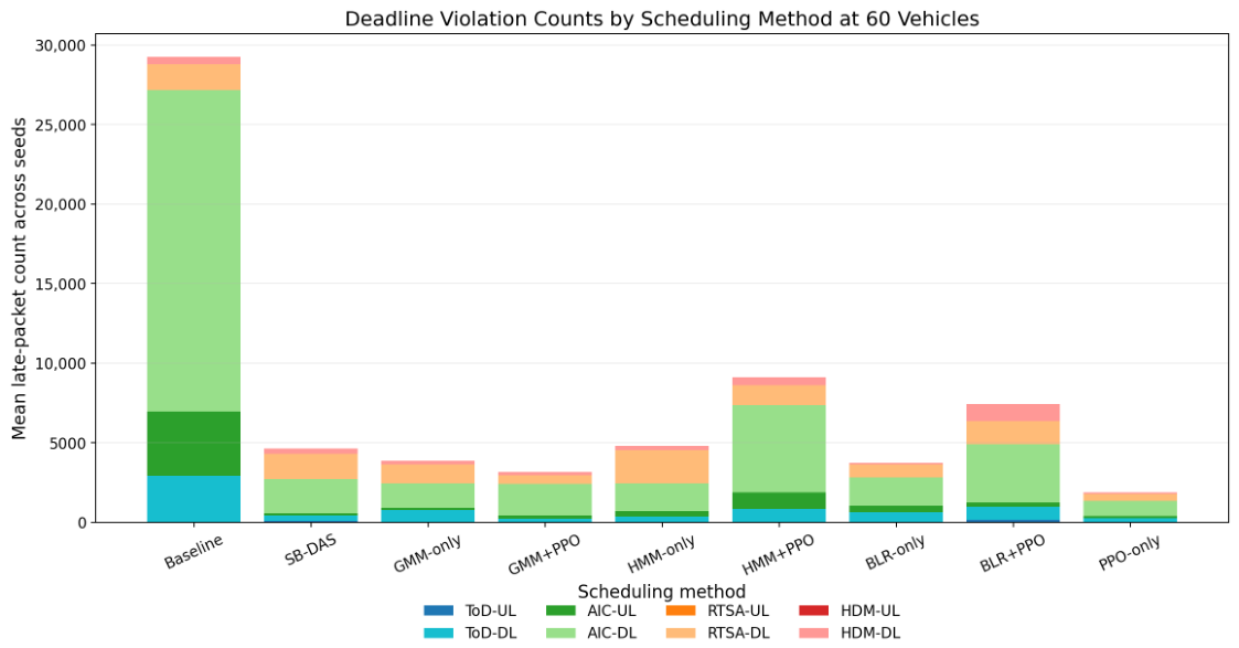
Figure 10 reports the absolute count of deadline violations at 60 vehicles, complementing DC-PRR by showing the magnitude of missed deadlines rather than only the normalized success ratio. The PF baseline produces by far the largest number of violations, dominated by the heavy uplink and downlink flows. All adaptive methods (SB-DAS and the AI-assisted variants) substantially reduce late packet delivery; the residual violations are concentrated in HDM-DL and RTSA-DL, consistent with the per-flow tables.

6.5. Secondary Metrics: Latency, Throughput, and Jitter

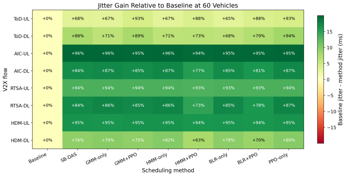
Although DC-PRR is the primary metric, the underlying delay distribution and throughput cost are also relevant. Table 12, Table 13, Table 14 and Table 15 report mean P95 latency, P99 latency, throughput, and jitter by vehicle density. The PF baseline degrades on every secondary metric as load increases: at 60 vehicles, its P95 latency reaches 148.3 ms, P99 latency 320.5 ms, jitter 16.7 ms, and normalized throughput drops to 0.73. Every adaptive method, including the non-learning SB-DAS heuristic, maintains higher throughput and substantially lower tail latency.
The classifier-only controllers and PPO-only maintain the most stable tail latency. HMM-only keeps P95 below 15 ms and jitter below 2 ms across all densities; GMM-only stays at or below 20 ms P95 (19.96 ms at 60 vehicles) with jitter below 2 ms. PPO-only achieves the lowest P95 at 60 vehicles (13.9 ms) and a P99 of 67.2 ms there. The non-learning SB-DAS heuristic tracks the classifier-only controllers on P95 (12–27 ms) and jitter (below 2.1 ms), although its P99 at 60 vehicles (139.8 ms) is higher than GMM-only and PPO-only. The classifier-assisted PPO variants show the largest tail-latency degradation as density increases (HMM+PPO P99 reaches 198.8 ms at 40 vehicles and BLR+PPO 151.6 ms at 60 vehicles), again indicating that the hybrid state representation is harder for the agent to exploit within the training budget.
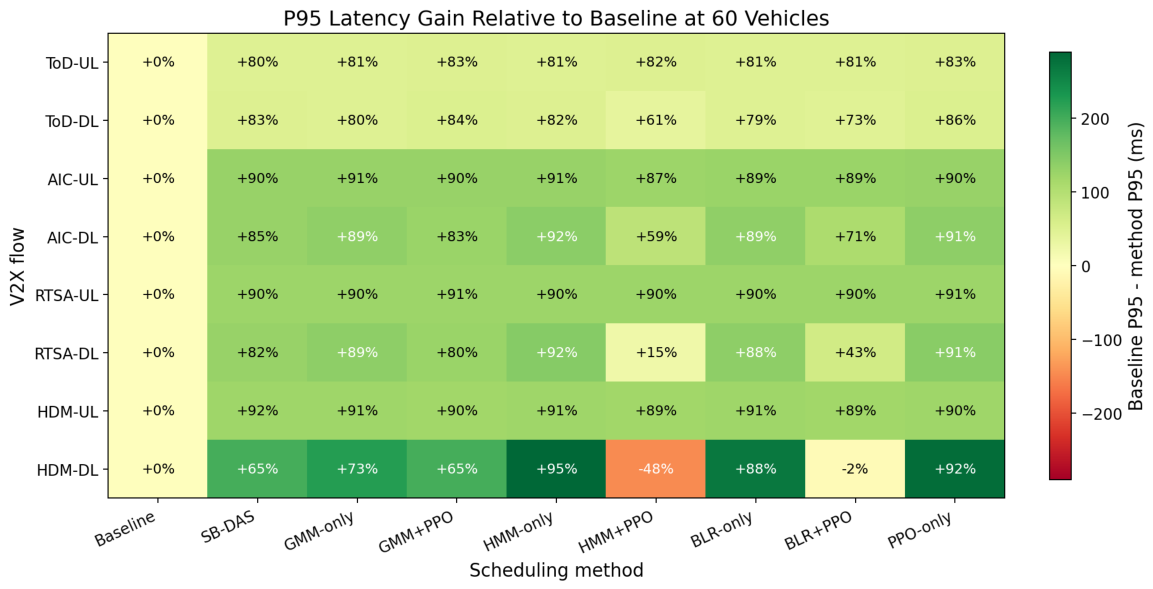
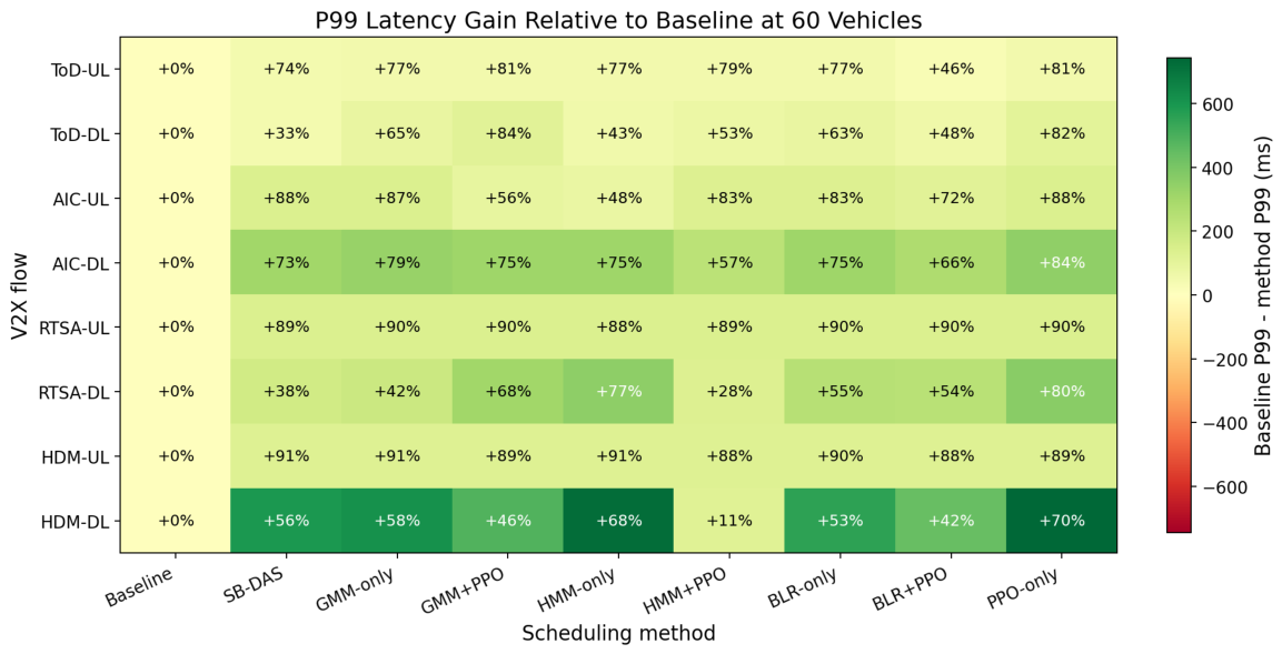
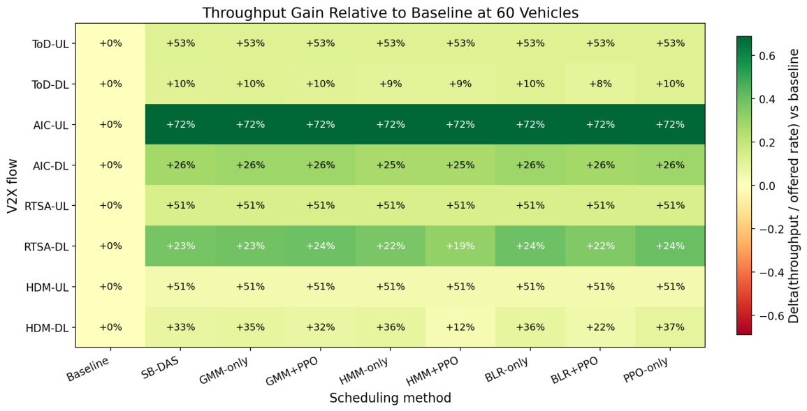
Figure 11, Figure 12, Figure 13 and Figure 14 provide per-flow heatmaps at 60 vehicles, showing where each method’s gains over PF are concentrated. The improvements are broad: most methods improve P95, P99, throughput, and jitter on most flows, with the largest absolute gains on the heavy uplink flows (ToD-UL, AIC-UL, RTSA-UL, HDM-UL) where PF was most badly degraded.

6.6. Scaling with Vehicle Density

Density behavior is summarized in the third column block of Table 6. The PF baseline degrades monotonically (75.2% → 65.3% → 44.1%). The non-learning SB-DAS heuristic is essentially flat across density (99.1% → 99.4% → 97.2%). The classifier-only methods are likewise flat: GMM-only stays above 97.5%, HMM-only between 98.1% and 98.7%, and BLR-only between 96.9% and 98.9%. PPO-only is also density-stable (98.7–99.8%). The classifier-assisted PPO variants show the largest density sensitivity, with HMM+PPO dropping from 99.4% at 30 vehicles to 91.2% at 60 vehicles.
Recall that the PPO policies were trained at 60 vehicles with +40% offered traffic. The 30- and 40-vehicle results therefore constitute zero-shot generalization tests: the agents were never exposed to these load levels during training. PPO-only generalizes well from the stressed training distribution to the lower-density evaluation conditions, and so do the GMM-only, HMM-only, and BLR-only controllers (which rely on classifiers trained on the same baseline data).

6.7. Comparing AI-Assisted Methods

Within the AI-assisted band, the methods clustered between 95.5% (HMM+PPO) and 99.1% (PPO-only). Three observations follow:
  • The differences are small relative to the seed variability. Mean differences of one to three percentage points between AI methods are comparable to or smaller than the across-seed standard deviations (Table 6). With three seeds per density, paired analyses cannot reliably separate methods that differ by less than two percentage points. For instance, the paired bootstrap confidence score for PPO-only exceeding GMM-only is only 67.5%, and the paired CI includes zero. PPO-only and GMM-only should therefore be regarded as statistically comparable at this sample size.
  • The hybrid PPO+classifier configurations did not deliver the expected benefit. Adding classifier-derived violation probabilities to the PPO state did not consistently improve performance: GMM+PPO underperformed both GMM-only and PPO-only; HMM+PPO showed the largest density sensitivity and the largest secondary-metric degradation; BLR+PPO sat between the standalone methods. This is a substantive negative finding for the privileged-feature design hypothesis. A plausible explanation is that PPO can extract equivalent information about deadline risk from the raw telemetry features in its state, so adding a classifier-derived probability is partially redundant. Further experimentation is needed to distinguish confidently between AI-assisted methods with statistically valid differences.
  • The robust comparative result is that all adaptive variants clearly outperform the PF baseline. Within the simulated load range, four learned/probabilistic controllers (GMM-only, HMM-only, BLR-only, PPO-only) form a tight performance band around 97.9–99.1% mean DC-PRR, and the non-learning SB-DAS heuristic falls inside the same band (Section 6.3). Three classifier-assisted PPO variants form a slightly broader and more variable band (95.5–98.1%). The main conclusion is that every adaptive variant, including the deterministic heuristic, consistently and clearly outperforms the PF baseline. Among the controllers, the practically interesting result is that GMM-only matches PPO-only within statistical noise, and SB-DAS in turn matches the learned controllers within statistical noise while being the simplest to train (it requires no training at all), deploy, and reason about.

6.8. Inference Latency and Computational Complexity

To ground the deployment-simplicity discussion (Section 7), we measured the per-control-cycle decision cost of each controller offline, by replaying representative telemetry through each method’s exact decision machinery (single-threaded, 1000 iterations, no ns-3/shared-memory overhead). Table 16 reports mean ± std per decision together with the big-O complexity, where F is the number of controlled flows (2 × UEs), U the served UEs, D = 19 features, and  K / S / M / H are model sizes.
SB-DAS is roughly one-to-four orders of magnitude cheaper per decision than the learned and probabilistic controllers and is essentially flat in density. Among the learned options, PPO-only and BLR-only are the lightest (about 0.13 ms per decision), GMM-only is heavier (about 0.7 ms) but still far below the budget, and the HMM-based variants are the most expensive (12–24 ms) owing to the O ( S 2 ) forward filtering; the hybrid PPO+classifier variants simply add the PPO forward pass on top of their classifier. Every method nevertheless stays well within the 100 ms control budget. Combined with the contribution analysis (Section 6.3), this places the deployment-simplicity claim on a measured footing: a rule-based deadline-aware controller obtains comparable DC-PRR at negligible inference cost, while among the learned controllers, PPO-only offers the best accuracy-to-cost ratio, matching GMM-only’s DC-PRR at roughly one-fifth of its per-decision cost.

6.9. Reward Contribution and Sensitivity

Because full PPO retraining under modified reward coefficients would require a substantially larger simulation budget, we provide a policy-fixed decomposition and one-at-a-time sensitivity analysis computed offline over the deployed policy’s recorded trajectories. Table 17 shows each reward term’s mean contribution and its share of the total reward signal. The slack and background terms dominate the signal, the altruism term is substantial, and the buffer-pressure penalty contributes a near-negligible share, consistent with the sensitivity sweep below.
A one-at-a-time coefficient sweep ( ± 25 / 50 % , policy and trajectory held fixed) ranks the coefficients by influence on the mean reward: the altruism gain is most influential (Δ mean reward ≈ 0.73 across the swept range), followed by the background gain (≈0.34), with the buffer-penalty weight least influential (≈0.016), again consistent with the small buffer-term share. We flag clearly that this analysis decomposes and rescales the reward over an already-trained policy’s trajectories rather than retraining; a fully retrained reward ablation is left to future work (Section 7).

7. Discussion

The central finding is that fairness-oriented PF scheduling is inadequate for mixed-criticality V2X traffic when delivery is evaluated under deadline constraints. PF DC-PRR falls to 44.1% at 60 vehicles in our simulations, with broad degradation across both critical and background flows. Lightweight deadline-aware adaptation of scheduler weights closes most of this gap: every adaptive variant we evaluated exceeded 95% mean DC-PRR and improved over PF in every paired density/seed comparison. This held across the non-learning SB-DAS heuristic, rule-based controllers driven by probabilistic classifiers, and a learned PPO policy. The SB-DAS baseline sharpens the interpretation: because a deterministic slack-and-violation rule on the same weight set reaches a DC-PRR statistically indistinguishable from the learned controllers (Section 6.3), the gain comes principally from the deadline-aware weight-adaptation principle itself rather than from a particular classifier or from learning. Within the evaluated scenarios and seed budget, learning did not provide a statistically resolvable DC-PRR gain over the strong SB-DAS heuristic, so we position the heuristic as a competitive, hard-to-beat reference rather than claiming an advantage for the learned controllers. The benefits a learned policy might still offer are adaptation to traffic or channel regimes not represented in our scenarios, transfer across deployments, or finer-grained control, which lie beyond what fixed-scenario, near-ceiling experiments can resolve, and we treat them as open questions for future evaluation rather than demonstrated advantages.
We deliberately do not claim a single best AI-assisted method or a strict ranking. Several considerations support this. First, the absolute differences between the top four controllers (GMM-only, HMM-only, BLR-only, PPO-only) are small relative to seed variability, and at n = 9 paired observations, the available statistical tests cannot resolve them. GMM-only achieves a result statistically indistinguishable from PPO-only while requiring no online exploration, no policy training infrastructure, and no learned-policy stability analysis. PPO-only achieves slightly higher P99 latency reduction and may adapt better when the traffic mix or channel conditions change in ways not captured by classifier features.
Our initial hypothesis was that augmenting PPO state with classifier-derived violation probabilities would yield privileged-feature gains beyond either component alone. GMM+PPO underperformed both GMM-only and PPO-only, while HMM+PPO showed the largest density sensitivity and the largest tail-latency degradation. BLR+PPO sat between the standalone methods. We interpret this as an important finding with two non-exclusive plausible mechanisms: (i) the raw telemetry already encodes most of the deadline-risk signal that the classifier extracts, so adding the probability is partially redundant, and (ii) adding a classifier feature increases the effective input dimensionality and slows learning within a bounded training budget.
Among the standalone classifiers, GMM produced the highest classifier-only DC-PRR. This is consistent with its offline behavior: it had the highest recall and ROC-AUC, at the cost of lower precision. For deadline-aware scheduling, false negatives (missing an at-risk flow) are more harmful than false positives (boosting a flow that did not need it), because the hysteresis-equipped weight-mapping rule absorbs short-term over-prioritization. HMM and BLR are more conservative; HMM’s low across-seed variance (standard deviation 0.27) reflects its temporal regime modeling and makes it the most stable classifier-only controller, which may be valuable in deployments that prioritize predictability over peak DC-PRR.

7.1. Deployment

The framework’s external-controller design makes it a natural fit for the O-RAN near-real-time RAN Intelligent Controller (near-RT RIC), where the proposed scheduler-weight adapter would be implemented as an xApp. The 100 ms control period sits well within the near-RT RIC’s 10 ms–1 s operating window, and the use of telemetry-driven weight adjustments (rather than scheduler replacement) maps cleanly onto the E2 interface’s existing scope: the xApp would consume per-UE radio and QoS measurements through E2SM-KPM-style indications and emit control actions via E2SM-RC policies that set per-UE priority weights at the gNB-DU MAC scheduler. The ns3-ai shared-memory link used here is the simulation analog of this control path. For deployment on a multi-access edge computing (MEC) host co-located with the gNB or RIC, inference cost is not a bottleneck: every controller’s per-decision cost is well below the 100 ms control period (Table 16), with the SB-DAS heuristic cheapest by one-to-four orders of magnitude, the GMM-only controller a small mixture model with sub-millisecond latency, and even the PPO policy a compact discrete-action network whose forward pass is well below the budget on commodity edge hardware. The non-learning and classifier-only variants are particularly attractive here because they require no online learning, produce deterministic outputs given the same telemetry, and are straightforward to certify and roll back, properties that matter for production xApp deployment more than peak DC-PRR.

7.2. Limitations

Several limitations affect the scope of our conclusions and should be noted.
  • Single-gNB topology due to tool constraints. The evaluation uses a single-cell deployment because the 5G-LENA NR module in ns-3 does not currently support handover. Multi-gNB scenarios with handover, inter-cell interference coordination, and multi-cell load balancing are therefore outside the scope of this study.
  • Compute-bounded PPO training. Each PPO training run requires more than two days of continuous wall-clock time because each control step calls a full ns-3 simulation step. PPO did not converge in a strict asymptotic sense within the available budget, and the PPO results should be interpreted as those of an online controller under fixed bounded training rather than of a fully converged policy. Longer training may improve policy quality, particularly for the classifier-assisted PPO variants, although inference results indicate a learned policy and improvement over the PF baseline.
  • Limited statistical power and inability of current experimental setup for ranking AI-assisted methods. With three seeds per density and method, the paired evidence is sufficient to support the primary PF-vs-adaptive comparison, because every adaptive method improved over PF in every matched density/seed pair with large effect sizes. However, distinguishing among the adaptive methods may require a more concentrated experimental design. Paired confidence scores and bootstrap CIs partially address this limitation, but absolute rankings among the top methods remain uncertain.
  • Discrete scheduler-weight action set. The action set W = { 1.0 , 2.0 , 5.0 , 10.0 } keeps the control problem tractable but may limit fine-grained adaptation. A continuous or finer-grained action space could improve performance but would require redesigning the classifier-only mapping rule, adapting the PPO action head, and, most importantly, using a much larger compute budget.
  • Open-loop sensitivity analyses. The reward-coefficient sensitivity and contribution decomposition (Section 6.9) and the weight-set sensitivity (Appendix B) were computed offline over recorded trajectories and decisions, with the policy and trajectory held fixed. They quantified how the reward/control signal responded to parameter changes but did not re-learn the policy. A fully retrained reward ablation and a closed-loop re-evaluation under alternative weight sets are left to future work due to the compute budget constraint.

8. Conclusions and Future Work

This paper presented a comparative study of probabilistic and reinforcement-learning controllers for deadline-aware MAC scheduler-weight adaptation in 5G NR V2X networks. The proposed closed-loop framework predicts imminent packet deadline violations from network telemetry every 100 ms, through GMM, HMM, or BLR classifiers and uses these predictions either directly via rule-based weight mapping or as state features for a PPO agent. The framework was implemented in ns-3 with the 5G-LENA NR module and ns3-ai shared memory and evaluated across three vehicle densities, three random seeds, and four V2X service classes against a PF baseline.
The main empirical findings were as follows: (i) the PF baseline achieved only 61.5% mean DC-PRR and degraded sharply with vehicle density, falling to 44.1% at 60 vehicles; (ii) every adaptive variant exceeded 95% mean DC-PRR and recovers 34–38 percentage points over PF in every paired density/seed comparison; (iii) the differences among the adaptive controllers were within seed-to-seed variability at three seeds per density, so we reported them as indicative rather than as a ranking and reserve significance claims for the PF-vs-adaptive gap; (iv) a non-learning Slack-Based Deadline-Aware Scheduler (SB-DAS) on the same weight set reached a DC-PRR statistically indistinguishable from the learned and probabilistic controllers, so based on the available evidence ( n = 9 paired observations), we found no statistically supported advantage of learning over the simple heuristic, we do not claim that learning is necessary or superior for this task, and we attribute most of the recovery over PF to deadline awareness rather than to learning; and (v) augmenting PPO state with classifier-derived violation probabilities did not consistently improve performance, indicating that the hybrid configuration did not earn its additional complexity in our setup.
The most practically interesting outcome is that lightweight deadline-aware control matches the learned policy in our experiments while remaining simpler and faster to deploy: the GMM-only variant matches PPO-only within statistical noise, and the training-free SB-DAS heuristic in turn matches the learned controllers within statistical noise at one-to-four orders of magnitude lower inference cost. We emphasize that our experiments do not establish that the learned or probabilistic controllers outperform the deterministic heuristic: the small mean differences fall within seed-to-seed variability and are not statistically resolvable at the evaluated sample size and experiment design. The simpler heuristic is the more parsimonious choice on the present evidence and learning would have to justify itself on grounds, robustness to distribution shift, transfer across scenarios, finer control, which lie beyond what this work evaluates. The robust scientific conclusion is that deadline-aware adaptive weighting, whether learned or not, closes the deadline-constrained delivery gap left by fairness-oriented PF scheduling.

Future Work

Future work will extend the evaluation in five directions. First, multi-gNB evaluation with handover is needed once 5G-LENA supports it, in order to assess inter-cell coordination and mobility-management effects. Second, a ranking-oriented methodology should be designed to distinguish near-ceiling AI-assisted controllers, including additional stress levels, repeated PPO training runs, and equivalence or non-inferiority testing. Third, the PPO formulation could be extended toward multi-agent reinforcement learning across cells, traffic classes, or network slices. Fourth, the discrete scheduler-weight action set could be replaced by a finer-grained or continuous control space. Finally, the ns3-ai control loop can be aligned with O-RAN concepts by mapping the external Python controller to a near-real-time RIC/xApp-style architecture.

Author Contributions

Conceptualization, G.P.-N.; methodology, G.P.-N.; software, G.P.-N.; validation, G.P.-N., D.N.S., A.K. (Athanasios Kanavos) and A.K. (Alexandros Kaloxylos); formal analysis, G.P.-N.; investigation, G.P.-N.; resources, G.P.-N.; data curation, G.P.-N.; writing—original draft preparation, G.P.-N.; writing—review and editing, G.P.-N., D.N.S., A.K. (Athanasios Kanavos) and A.K. (Alexandros Kaloxylos); visualization, G.P.-N.; supervision, G.P.-N. and D.N.S.; project administration, G.P.-N. and D.N.S. All authors have read and agreed to the published version of the manuscript.

Funding

This research received no external funding.

Institutional Review Board Statement

Not applicable.

Informed Consent Statement

Not applicable.

Data Availability Statement

The original contributions presented in this study are included in the article. Further inquiries can be directed to the corresponding author.

Acknowledgments

The authors acknowledge the use of ns-3, the 5G-LENA NR module, SUMO, and ns3-ai in the development and evaluation of the simulation framework. The authors acknowledge the use of GenAI (ChatGPT—GPT-5.5 Instant) during the editing and revision phase of this manuscript text to improve readability and language quality.

Conflicts of Interest

The authors declare no conflicts of interest.

Appendix A. Consolidated Notation and Parameter Table

Table A1 defines every symbol, threshold, and constant used in the slack, reward, and weight-mapping equations, providing a single reference for the equation audit.
Table A1. Symbols, constants, and thresholds used in the scheduler-mapping and reward equations.
Symbol/ConstantMeaningValue/Domain
iUE (or flow) index
tControl-cycle index (period 100 ms)
D i Packet deadline for UE ims
L i ( t ) Observed latencyms
s i ( t ) Minimum remaining slack = D i L i ( t ) ms
v i ( t ) Recent deadline-violation ratio (5-cycle window) [ 0 , 1 ]
i ( t ) Discrete priority level { 1 , 2 , 3 , 4 }
w i ( t ) Applied scheduler weight = map ( ) { 1 , 2 , 5 , 10 }
H ( t ) Mean critical-UE health [ 0 , 1 ]
b i Buffer occupancy normalized to capacity [ 0 , 1 ]
Control periodAll controllers100 ms
Rolling windowFeature/violation window5 cycles (500 ms)
Deadlines ToD UL/DLSlack, DC-PRR100/20 ms
Deadlines AIC UL/DLSlack, DC-PRR100/100 ms
Deadlines RTSA UL/DLDC-PRR500/500 ms
Deadlines HDM UL/DLDC-PRR1000/1000 ms
Weight map w Scheduler 1 1 , 2 2 , 3 5 , 4 10
SB-DAS slack edgesLevel rule50/20/5 ms
SB-DAS violation-ratio thresholdLevel rule0.2
SB-DAS hysteresis marginDowngrade guard5 ms
Classifier thresholds θ 1 , θ 2 , θ 3 level quantization0.30/0.60/0.85
Classifier L4 hysteresis holdLevel hold3 cycles (300 ms)
GMM components KClassifier5 (diag. cov.)
HMM states SClassifier8 (diag. cov.) + LR head
BLR prior precision/MC samples MClassifier1.0/100
ToD/AIC buffer capacityBuffer normalization256/64 KiB

Appendix B. Scheduler-Weight-Set Sensitivity

We compared the default set { 1 , 2 , 5 , 10 } against { 1 , 2 , 4 , 8 } (octave) and { 1 , 3 , 6 , 10 } (more linear) by replaying the recorded SB-DAS level decisions and re-mapping levels to each set. Because SB-DAS selects the L1–L4 level from telemetry independently of the numeric weights, the level mix is fixed and only the applied weight value changes (Table A2).
Table A2. Open-loop weight-set sensitivity: the recorded SB-DAS level mix (L1 89.1%, L2 0.4%, L3 5.9%, L4 4.6%) re-mapped onto each weight set. The level decisions are identical across sets, so only the applied weight changes.
Weight SetMean Applied Weightp95 Applied WeightBoosted Weight-Mass %
{ 1 , 2 , 5 , 10 } (default)1.654546.1
{ 1 , 2 , 4 , 8 } (octave)1.503440.7
{ 1 , 3 , 6 , 10 } (linear)1.716648.1
The weight set rescales the priority signal but does not change which flows are prioritized. The default { 1 , 2 , 5 , 10 } provides the strongest normal-vs-emergency contrast ( 10 × ) while retaining four interpretable levels; { 1 , 2 , 4 , 8 } weakens the emergency boost to 8 × , and  { 1 , 3 , 6 , 10 } mainly raises the mild/strong boosts. This is an open-loop analysis (fixed recorded decisions); a closed-loop re-evaluation under alternative sets would require re-simulation and is left to future work.

Appendix C. SB-DAS Threshold Sensitivity

To check whether the SB-DAS result depended on careful tuning of its slack edges and violation threshold, we replayed 282,240 recorded critical-flow decisions through the rule with each threshold swept one at a time (background flows are fixed at L1 by construction and therefore omitted from the sweep; hysteresis is stateful and therefore not modeled in this static replay). Table A3 reports the boosted fraction P ( > 1 ) and the mean applied weight at each setting. Over wide ranges of all four thresholds, the boosted fraction moves by less than ± 1  pp, indicating that the heuristic is not finely tuned: its decisions are stable to threshold perturbation. The single exception is raising the “safe” slack edge to 100 ms, which reclassifies almost all traffic as mildly urgent because 100 ms exceeds most observed slack values. As with the other open-loop analyses, changing a threshold in a live run would alter subsequent scheduling and hence the observed slack (a closed-loop feedback effect not captured here), so these figures quantify how the rule reacts to its inputs rather than an end-to-end metric change.
Table A3. Open-loop SB-DAS threshold sensitivity (recorded-decision replay). Boosted fraction P ( > 1 ) and mean applied weight; one threshold swept at a time, others at default. * = default.
ThresholdValueBoosted % ( > 1 )Mean Weight
SLACK_SAFE_MS3010.571.641
50 *10.861.644
7011.781.653
100100.02.536
SLACK_MILD_MS1010.861.483
20 *10.861.644
4010.861.650
SLACK_HIGH_MS210.861.642
5 *10.861.644
1510.861.944
VIOL_RATIO_THR0.111.371.697
0.2 *10.861.644
0.810.731.630

Appendix D. Reproducibility and Implementation Parameters

This appendix lists the software versions and per-method coefficients needed to reproduce the experiments. The radio and traffic configuration is given in Table 1 and Table 2 (25 MHz channel bandwidth, numerology two, 60 kHz subcarrier spacing, RLC AM); the level → weight map is in Table A1.
Table A4. Software and toolchain versions.
ComponentVersion/Reference
ns-33.46.1 (dev), git ns-3.46
nr (5G-LENA)v4.1.1 (contrib/nr)
ns3-aigit b8c9858 (contrib/ai)
Build profileoptimized (-d optimized, release)
Compiler/CMakegcc 13.3.0/CMake 3.28.3
OS/kernelUbuntu 24.04.4 LTS/6.17.0-35-generic
Python3.11.14 (conda env ns3ai_env)
numpy/pandas/scipy2.3.5/2.3.3/1.17.0
torch2.9.1+cu128
scikit-learn/hmmlearn1.8.0/0.3.3
optuna/matplotlib/joblib4.8.0/3.10.7/1.5.3
Table A5. SB-DAS constants.
ConstantValue
SLACK_SAFE_MS50
SLACK_MILD_MS20
SLACK_HIGH_MS5
VIOLATION_RATIO_THRESHOLD0.2
HYSTERESIS_SLACK_MS5
CONTROL_CYCLE_S0.1
WINDOW_SAMPLES5
The remaining per-controller configuration details are as follows:
1.
Background flows. HDM/RTSA flows are clamped to L1.
2.
Classifier-only common quantization. Probability thresholds [ 0.30 , 0.60 , 0.85 ] L2/L3/L4 (else L1); L4 hysteresis hold three cycles; 100 ms control cycle; five-sample rolling feature window. Per-classifier: GMM two class-conditional models, n_components=5, diag. cov., reg_covar=1e-4; HMM n_components=8, diag. cov., logistic head C = 1.0 , online forward filtering; BLR prior_precision=1.0, n_mc_samples=100, Laplace approximation.
3.
PPO hyperparameters (shared across all PPO variants). Learning rate: 8.139 × 10 4 ; discount: γ = 0.9019 ; GAE: λ = 0.9089 ; clip ϵ = 0.0578 ; entropy coef. 0.0206 ; value-loss coef. 0.5 ; max grad norm: 0.5 ; rollout length: 32; PPO epochs: four; mini-batch: 32; network shared: 19 256 256 (ReLU), actor: 256 128 4 , critic: 256 128 1 ; action → level map: [ 4 , 3 , 2 , 1 ] ; shield emergency-slack threshold: 5 ms. Training used a 500 s trace at 60-vehicle density with + 40 % offered load; evaluation seeds: one, two, three; densities: 30, 40, 60.

References

  1. TS 22.186; Service Requirements for Enhanced V2X Scenarios (Release 16). Technical Specification 22.186. 3rd Generation Partnership Project (3GPP): Valbonne, France, 2019.
  2. Bagheri, H.; Noor-A-Rahim, M.; Liu, Z.; Lee, H.; Pesch, D.; Moessner, K.; Xiao, P. 5G NR-V2X: Toward Connected and Cooperative Autonomous Driving. IEEE Commun. Stand. Mag. 2021, 5, 48–54. [Google Scholar] [CrossRef]
  3. Capozzi, F.; Piro, G.; Grieco, L.A.; Boggia, G.; Camarda, P. Downlink Packet Scheduling in LTE Cellular Networks: Key Design Issues and a Survey. IEEE Commun. Surv. Tutor. 2013, 15, 678–700. [Google Scholar] [CrossRef]
  4. Patriciello, N.; Lagén, S.; Bojović, B.; Giupponi, L. An E2E Simulator for 5G NR Networks. Simul. Model. Pract. Theory 2019, 96, 101933. [Google Scholar] [CrossRef]
  5. Liang, L.; Ye, H.; Li, G.Y. Spectrum Sharing in Vehicular Networks Based on Multi-Agent Reinforcement Learning. IEEE J. Sel. Areas Commun. 2019, 37, 2282–2292. [Google Scholar] [CrossRef]
  6. Ye, H.; Li, G.Y.; Juang, B.H.F. Deep Reinforcement Learning Based Resource Allocation for V2V Communications. IEEE Trans. Veh. Technol. 2019, 68, 3163–3173. [Google Scholar] [CrossRef]
  7. Shao, Z.; Wu, Q.; Fan, P.; Cheng, N.; Fan, Q.; Wang, J. Semantic-Aware Resource Allocation Based on Deep Reinforcement Learning for 5G-V2X HetNets. arXiv 2024, arXiv:2406.07996. [Google Scholar]
  8. Jabeen, S. A Deep Reinforcement Learning Based Scheduler for IoT Devices in Co-existence with 5G-NR. arXiv 2025, arXiv:2501.11574. [Google Scholar]
  9. AL-Tam, F.; Correia, N.; Rodriguez, J. Learn to Schedule (LEASCH): A Deep Reinforcement Learning Approach for Radio Resource Scheduling in the 5G MAC Layer. IEEE Access 2020, 8, 108088–108101. [Google Scholar] [CrossRef]
  10. Gu, Z.; She, C.; Hardjawana, W.; Lumb, S.; McKechnie, D.; Essery, T.; Vucetic, B. Knowledge-Assisted Deep Reinforcement Learning in 5G Scheduler Design: From Theoretical Framework to Implementation. IEEE J. Sel. Areas Commun. 2021, 39, 2014–2028. [Google Scholar] [CrossRef]
  11. Sun, S.; Li, X. Deep-Reinforcement-Learning-Based Scheduling with Contiguous Resource Allocation for Next-Generation Wireless Systems. In Proceedings of the Intelligent Computing; Lecture Notes in Networks and Systems; Springer: Cham, Switzerland, 2021; Volume 285, pp. 637–657. [Google Scholar] [CrossRef]
  12. Barmpounakis, S.; Maroulis, N.; Koursioumpas, N.; Kousaridas, A.; Kalamari, A.; Kontopoulos, P.; Alonistioti, N. AI-Driven QoS Prediction for V2X Communications in Beyond 5G Systems. Comput. Netw. 2022, 217, 109341. [Google Scholar] [CrossRef]
  13. Palaios, A.; Vielhaus, C.L.; Külzer, D.F.; Watermann, C.; Hernangomez, R.; Partani, S.; Geuer, P.; Krause, A.; Sattiraju, R.; Kasparick, M.; et al. Machine Learning for QoS Prediction in Vehicular Communication: Challenges and Solution Approaches. IEEE Access 2023, 11, 92459–92477. [Google Scholar] [CrossRef]
  14. Koursioumpas, N.; Magoula, L.; Stavrakakis, I.; Alonistioti, N.; Gutierrez-Estevez, M.A.; Khalili, R. DISTINQT: A Distributed Privacy Aware Learning Framework for QoS Prediction for Future Mobile and Wireless Networks. arXiv 2024, arXiv:2401.10158. [Google Scholar]
  15. Allahdadi, A.; Morla, R. Anomaly Detection and Modeling in 802.11 Wireless Networks. J. Netw. Syst. Manag. 2019, 27, 3–38. [Google Scholar] [CrossRef]
  16. TS 23.501; System Architecture for the 5G System (5GS) (Release 17). Technical Specification 23.501. 3rd Generation Partnership Project (3GPP): Valbonne, France, 2022.
  17. Liu, C.L.; Layland, J.W. Scheduling Algorithms for Multiprogramming in a Hard-Real-Time Environment. J. ACM 1973, 20, 46–61. [Google Scholar] [CrossRef]
  18. Andrews, M.; Kumaran, K.; Ramanan, K.; Stolyar, A.; Vijayakumar, R.; Whiting, P. Providing Quality of Service over a Shared Wireless Link. IEEE Commun. Mag. 2001, 39, 150–154. [Google Scholar] [CrossRef]
  19. Hendaoui, S.; Hendaoui, F.; Zangar, N. Dynamic Proactive–Reactive Scheduling for URLLC in 5G: Leveraging XGBoost and Network Virtualization. Phys. Commun. 2025, 68, 102553. [Google Scholar] [CrossRef]
  20. Cohen, K.M.; Park, S.; Simeone, O.; Popovski, P.; Shamai, S. Guaranteed Dynamic Scheduling of Ultra-Reliable Low-Latency Traffic via Conformal Prediction. IEEE Signal Process. Lett. 2023, 30, 473–477. [Google Scholar] [CrossRef]
  21. Robaglia, B.M.; Destounis, A.; Coupechoux, M.; Tsilimantos, D. Deep Reinforcement Learning for Scheduling Uplink IoT Traffic with Strict Deadlines. In Proceedings of the IEEE Global Communications Conference (GLOBECOM), Madrid, Spain, 7–11 December 2021; IEEE: Piscataway, NJ, USA, 2021; pp. 1–6. [Google Scholar]
  22. Kanavos, A.; Barmpounakis, S.; Kaloxylos, A. An Adaptive Scheduling Mechanism Optimized for V2N Communications over Future Cellular Networks. Telecom 2023, 4, 378–392. [Google Scholar] [CrossRef]
  23. Alshiekh, M.; Bloem, R.; Ehlers, R.; Könighofer, B.; Niekum, S.; Topcu, U. Safe Reinforcement Learning via Shielding. Proc. AAAI Conf. Artif. Intell. 2018, 32, 2669–2678. [Google Scholar] [CrossRef]
  24. Carr, S.; Jansen, N.; Junges, S.; Topcu, U. Safe Reinforcement Learning via Shielding under Partial Observability. Proc. AAAI Conf. Artif. Intell. 2023, 37, 14748–14756. [Google Scholar] [CrossRef]
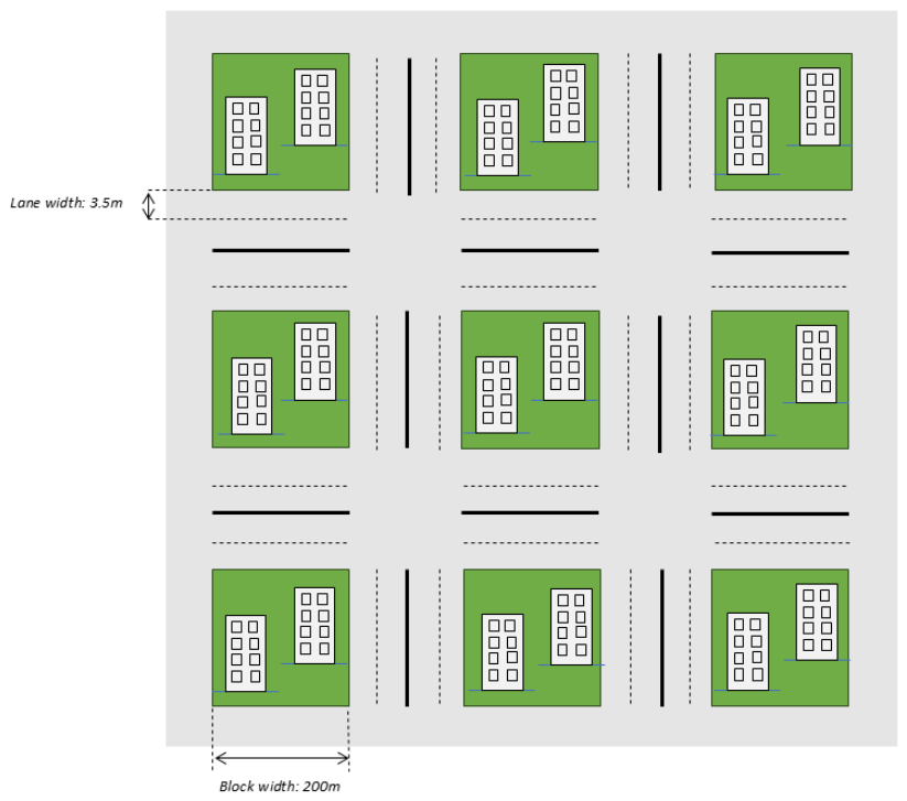
Figure 1. SUMO-generated Manhattan-grid mobility scenario used for the simulated urban V2X deployment.
Telecom 07 00080 g001
Figure 2. Closed-loop control architecture. The ns3-ai shared-memory interface bridges the ns-3 simulator (containing the NR TDMA QoS scheduler) and the external Python control agent, which selects per-UE scheduler weights every 100 ms using one of three control modes (SB-DAS, classifier-only, or PPO).
Telecom 07 00080 g002
Figure 3. GMM feature-space representation of deadline-violation behavior. The mixture components capture different network operating regimes, including safe and violation-prone regions.
Telecom 07 00080 g003
Figure 4. Standardized feature profiles of the learned GMM components.
Telecom 07 00080 g004
Figure 5. HMM hidden-state transition matrix. The model captures persistent healthy and congestion regimes, as well as a transient warning state before congestion.
Telecom 07 00080 g005
Figure 6. BLR confidence distribution for deadline-violation prediction.
Telecom 07 00080 g006
Figure 7. Mean PPO training reward for the evaluated PPO variants.
Telecom 07 00080 g007
Figure 8. PPO policy loss during training.
Telecom 07 00080 g008
Figure 9. Approximate KL divergence during PPO training. Bounded values confirm that PPO clipping prevented excessively large policy updates.
Telecom 07 00080 g009
Figure 10. Deadline violation counts at 60 vehicles. Bars are stacked by V2X flow.
Telecom 07 00080 g010
Figure 11. P95 latency gain relative to the PF baseline by V2X flow and scheduling method at 60 vehicles. Positive values indicate reduced P95 latency.
Telecom 07 00080 g011
Figure 12. P99 latency gain relative to the PF baseline by V2X flow and scheduling method at 60 vehicles.
Telecom 07 00080 g012
Figure 13. Throughput gain relative to the PF baseline by V2X flow and scheduling method at 60 vehicles.
Telecom 07 00080 g013
Figure 14. Jitter gain relative to the PF baseline by V2X flow and scheduling method at 60 vehicles. Positive values indicate more stable timing.
Telecom 07 00080 g014
Table 1. 5G NR radio configuration used in the simulation.
ParameterValue
Simulatorns-3 with 5G-LENA NR module
DeploymentSingle-gNB urban V2X cell
Carrier frequency4 GHz
System bandwidth25 MHz
Numerology2
Subcarrier spacing60 kHz
MAC schedulerNR TDMA QoS scheduler
RLC modeAM
Mobility sourceSUMO Manhattan-grid traces
AI interfacens3-ai shared memory
Control period100 ms
Table 2. V2X traffic configuration.
FlowDirectionPacket SizePeriodOffered Rate
HDMDL1200 B3 ms3.20 Mbps
HDMUL600 B10 ms0.48 Mbps
AICDL1000 B10 ms0.80 Mbps
AICUL1200 B10 ms0.96 Mbps
ToDDL600 B10 ms0.48 Mbps
ToDUL1200 B3 ms3.20 Mbps
RTSADL1000 B10 ms0.80 Mbps
RTSAUL1000 B10 ms0.80 Mbps
Table 3. Reward-function coefficients and constants (source of truth: the deployed PPO agents). A reward-contribution and coefficient-sensitivity analysis is given in Section 6.9.
SymbolValueRole/Where It Enters
Violation penalty multiplier3.0Negative branch of R slack
Positive-slack saturation1.0tanh upper bound ( s 0 )
Buffer-pressure weight (UL, DL)1.0 each ( b ul + b dl ) , critical UEs
Background rescale gain4.0 4 target 2
Background rescale offset 2.0 4 target 2
Altruism gain2.0 2 H 1
Altruism offset 1.0 2 H 1
ToD buffer capacity256 KiB b cap (ToD)
AIC buffer capacity64 KiB b cap (AIC)
ToD deadline (UL/DL)100/20 msSlack normalizer D
AIC deadline (UL/DL)100/100 msSlack normalizer D
Table 4. Optuna hyperparameter search results for PPO training.
TrialScoreElapsed (s)LR γ λ ϵ Rollout
90.99998057.50.0008140.90190.90890.057832
10.99788043.20.0000250.99070.97060.1402128
70.99748059.10.0001030.94350.98720.165532
50.99668040.40.0001500.90540.98740.194664
40.99398001.40.0000400.95010.93650.1197128
20.99157975.20.0004570.92580.96010.068332
80.98938010.10.0000330.92190.91990.167432
60.98458020.10.0007370.90810.90340.2027256
00.97168024.40.0000240.94480.98340.102964
30.93437764.70.0004330.96640.93850.224064
Table 5. Offline classifier performance for next-window deadline-violation prediction.
ClassifierAccuracyF1PrecisionRecallROC-AUCAvg. Prec.ECE
GMM0.93660.77090.70890.84670.95440.8157
HMM0.94080.71560.90170.59330.92560.8199
BLR0.94050.71400.90100.59150.92840.82200.0225
Table 6. Mean DC-PRR (%) by scheduling method and vehicle density, including the non-learning SB-DAS baseline. Overall values are aggregated across all densities and random seeds.
Method30 Veh.40 Veh.60 Veh.OverallStd.95% CI
PF baseline75.2065.3344.1161.5514.54[52.37, 70.21]
SB-DAS99.1499.3997.2298.581.51[97.56, 99.35]
GMM-only99.6299.7797.5398.971.11[98.25, 99.64]
HMM-only98.3398.7098.1198.380.28[98.21, 98.53]
BLR-only97.7898.9596.9397.891.61[96.78, 98.73]
GMM+PPO98.8597.8297.6798.111.40[97.09, 98.86]
HMM+PPO99.4095.8391.1895.476.89[90.73, 98.48]
BLR+PPO98.5797.2793.9496.594.52[93.48, 98.67]
PPO-only99.7798.6998.8299.090.73[98.63, 99.54]
PPO-only+shield98.5797.0196.0497.212.34[95.70, 98.52]
Table 7. Paired DC-PRR improvement over the PF baseline across the nine density/seed pairs. The confidence score is the bootstrap-estimated probability that the method improves mean DC-PRR over PF.
MethodMean Gain95% CI Low95% CI HighConf.Wilcoxon
(pp)(pp)(pp)Score p
SB-DAS37.0428.8545.61100%0.00195
GMM-only37.4329.1746.02100%0.00195
HMM-only36.8328.1345.78100%0.00195
BLR-only36.3427.7945.38100%0.00195
GMM+PPO36.5728.4845.29100%0.00195
HMM+PPO33.9226.5742.03100%0.00195
BLR+PPO35.0527.1543.68100%0.00195
PPO-only37.5528.9046.65100%0.00195
PPO-only+shield35.6627.2844.34100%0.00195
Table 8. Method-component contribution ladder: DC-PRR (%) and incremental gain (Δpp over the rung above), per density. Incremental gains are computed from unrounded run-level values and may therefore differ from differences of the rounded DC-PRR entries by up to ±0.01 pp.
Rung30 Veh.40 Veh.60 Veh.
PF baseline75.2065.3344.11
SB-DAS99.14 (+23.94)99.39 (+34.05)97.22 (+53.12)
GMM-only99.62 (+0.48)99.77 (+0.39)97.53 (+0.31)
GMM+PPO98.85 (−0.76)97.82 (−1.96)97.67 (+0.14)
PPO-only+shield98.57 (−0.28)97.01 (−0.81)96.04 (−1.63)
Table 9. DC-PRR (%) by V2X flow at 30 vehicles for all evaluated scheduling methods.
FlowPFSB-DASGMM-OnlyHMM-OnlyBLR-OnlyGMM+PPOHMM+PPOBLR+PPOPPO-OnlyPPO+Shield
ToD-UL99.9999.8399.8799.7099.6199.7199.9999.9099.9099.90
ToD-DL95.2199.6599.6299.0697.8699.82100.0099.93100.0099.93
AIC-UL42.6296.8299.3495.9886.0292.6596.0281.4298.5381.42
AIC-DL98.3999.7399.6598.9899.0499.75100.0099.9699.9899.96
RTSA-UL46.5499.8299.7999.9299.5399.8999.9299.4399.9999.43
RTSA-DL98.6699.7699.5497.6998.8899.64100.0099.9699.9999.96
HDM-UL63.11100.00100.00100.00100.00100.00100.00100.0099.98100.00
HDM-DL98.9399.7299.3496.6597.8399.2099.9999.8599.9399.85
Table 10. DC-PRR (%) by V2X flow at 40 vehicles.
FlowPFSB-DASGMM-OnlyHMM-OnlyBLR-OnlyGMM+PPOHMM+PPOBLR+PPOPPO-OnlyPPO+Shield
ToD-UL99.9399.9599.9899.7199.8199.9999.2499.9699.9899.99
ToD-DL96.2399.5899.7998.2699.1797.7695.8297.4098.9996.68
AIC-UL24.9199.7299.8499.4598.1599.3899.5896.6499.7297.89
AIC-DL87.4699.3299.7698.3099.2697.3395.5796.9998.8796.59
RTSA-UL39.0799.8699.9599.9598.9799.9399.6899.9299.3499.88
RTSA-DL89.5298.9999.7697.5399.0296.1091.8096.0998.2694.61
HDM-UL25.91100.00100.00100.00100.0099.9999.99100.0099.97100.00
HDM-DL95.3997.8498.9496.4598.3392.6587.2892.7594.7792.42
Table 11. DC-PRR (%) by V2X flow at 60 vehicles.
FlowPFSB-DASGMM-OnlyHMM-OnlyBLR-OnlyGMM+PPOHMM+PPOBLR+PPOPPO-OnlyPPO+Shield
ToD-UL44.4499.5999.6699.7493.5599.9699.9799.5399.9399.83
ToD-DL78.1397.2697.4596.6897.2498.2091.6494.3898.8695.18
AIC-UL23.1499.7898.6499.7096.8599.7798.5699.7199.7699.78
AIC-DL54.6696.7598.0596.9797.8497.1789.6893.6198.5795.12
RTSA-UL35.3599.9298.5999.9098.2999.9599.9199.9799.9699.92
RTSA-DL54.4495.0596.3596.5496.7496.1080.1887.0197.9691.98
HDM-UL33.9199.99100.00100.00100.0099.9999.9599.9799.9999.97
HDM-DL54.9289.6892.1894.9094.0389.5072.6782.2495.4187.40
Table 12. Mean P95 latency (ms) by vehicle density.
Method30 Veh.40 Veh.60 Veh.
PF baseline71.9798.50148.29
SB-DAS14.2212.2426.50
GMM-only11.1911.4419.96
HMM-only14.9111.7112.64
BLR-only19.0012.0817.17
GMM+PPO15.8822.7726.69
HMM+PPO13.5834.1675.11
BLR+PPO18.1328.8770.09
PPO-only10.8919.3013.89
PPO-only+shield18.1331.3032.21
Table 13. Mean P99 latency (ms) by vehicle density.
Method30 Veh.40 Veh.60 Veh.
PF baseline103.14132.20320.50
SB-DAS22.1742.07139.78
GMM-only19.3919.68123.88
HMM-only69.4071.3285.17
BLR-only38.6731.84118.21
GMM+PPO28.51114.55112.76
HMM+PPO15.39198.77175.00
BLR+PPO27.5699.26151.59
PPO-only19.6751.6667.17
PPO-only+shield27.56139.89227.35
Table 14. Mean normalized throughput by vehicle density. Throughput is normalized to the nominal per-flow offered load; values slightly above 1.0 reflect delivery of traffic that was queued during earlier congested intervals (backlog drainage), so the delivered total within a measurement window can briefly exceed the instantaneous offered total.
Method30 Veh.40 Veh.60 Veh.
PF baseline0.9160.8750.733
SB-DAS1.0231.0271.016
GMM-only1.0271.0271.021
HMM-only1.0221.0221.017
BLR-only1.0191.0271.022
GMM+PPO1.0261.0201.020
HMM+PPO1.0271.0111.002
BLR+PPO1.0221.0201.004
PPO-only1.0271.0241.024
PPO-only+shield1.0221.0161.010
Table 15. Mean jitter (ms) by vehicle density.
Method30 Veh.40 Veh.60 Veh.
PF baseline7.6310.8416.72
SB-DAS0.941.182.04
GMM-only0.831.021.87
HMM-only1.221.161.79
BLR-only1.631.142.01
GMM+PPO1.241.721.93
HMM+PPO1.041.803.00
BLR+PPO1.592.242.48
PPO-only0.801.491.65
PPO-only+shield1.591.912.10
Table 16. Per-control-cycle inference latency and computational complexity by method. Offline micro-benchmark (single-threaded, 1000 iterations, no ns-3/shared-memory overhead); every method stays within the 100 ms control budget. Cells report mean ± std/p95 in ms. Here F is the number of controlled flows (2 × UEs), U the served UEs, D = 19 features, K = 5 GMM components, S = 8 HMM states, M = 100 BLR Monte-Carlo samples, and H the PPO hidden width.
MethodComplexityParams30 Vehicles40 Vehicles60 Vehicles
PF baseline— (no control loop)nonen/an/an/a
SB-DAS O ( F ) 00.0060 ± 0.0004/0.00610.0056 ± 0.0001/0.00570.0058 ± 0.0001/0.0059
GMM-only O ( F K D ) 60960.6703 ± 0.0202/0.68230.6893 ± 0.0108/0.71140.7167 ± 0.0110/0.7444
HMM-only O ( F S 2 ) 156411.7808 ± 0.1358/11.997216.2086 ± 0.0905/16.338423.4847 ± 0.1921/23.6609
BLR-only O ( F D M ) 4200.1268 ± 0.0099/0.13390.1314 ± 0.0090/0.13740.1374 ± 0.0043/0.1440
PPO-only O ( U H 2 ) 135,5570.1228 ± 0.0018/0.12460.1478 ± 0.0073/0.15270.1923 ± 0.0031/0.1971
GMM+PPO O ( F K D + U H 2 ) 141,6530.8522 ± 0.0302/0.88610.9161 ± 0.0438/0.97190.9752 ± 0.0126/0.9960
HMM+PPO O ( F S 2 + U H 2 ) 137,12112.0662 ± 0.1272/12.241416.3170 ± 0.1535/16.585224.1710 ± 0.2201/24.4745
BLR+PPO O ( F D M + U H 2 ) 135,9770.2849 ± 0.0122/0.29720.3185 ± 0.0073/0.33160.3734 ± 0.0071/0.3851
Table 17. Reward-term contribution over the deployed PPO trajectories (policy-fixed, offline).
Reward TermMean ContributionShare of Signal
Background 0.58 35.8%
Slack + 0.34 33.9%
Altruism + 0.46 28.3%
Buffer penalty 0.03 2.0%
Disclaimer/Publisher’s Note: The statements, opinions and data contained in all publications are solely those of the individual author(s) and contributor(s) and not of MDPI and/or the editor(s). MDPI and/or the editor(s) disclaim responsibility for any injury to people or property resulting from any ideas, methods, instructions or products referred to in the content.