Phased Antenna-Array Synthesis Using Taylor-Series Expansion and Neural Networks

Abstract

This paper presents a novel approach to synthesizing phased antenna arrays (PAAs) by combining Taylor-series expansion with neural networks (NNs), enhancing the PAA synthesis process for modern communication and radar systems. Synthesizing PAAs is crucial for these systems, offering versatile beamforming capabilities. Traditional methods often rely on complex analytical formulations or numerical optimizations, leading to suboptimal solutions or high computational costs. The proposed method uses Taylor-series expansion to derive analytical expressions for PAA radiation patterns and beamforming characteristics, simplifying the optimization process. Additionally, neural networks are employed to model the intricate relationships between PAA parameters and desired performance metrics, providing adaptive learning and real-time adjustments. A validation of the proposed method is performed on a dual-band 5G antenna, which exhibits marked resonances at 28.14 GHz and 37.88 GHz, with reflection coefficients of $S_{11}$ = −19 dB and $S_{11}$ = −19.33 dB, respectively. The integration of Taylor expansion with NNs offers improved efficiency, reduced computational complexity, and the ability to explore a broader design space. Simulation results and case studies demonstrate the effectiveness and applicability of the approach in practical scenarios. This work represents a significant advancement in PAA synthesis, showcasing the synergistic integration of mathematical modeling and artificial intelligence for optimized antenna design in modern communication and radar systems.

1. Introduction

The integration of the Taylor method with neural networks in antenna array design signifies a sophisticated synergy between mathematical modeling and computational learning, yielding unprecedented levels of precision and adaptability. Unlike Chebyshev- or Fourier-based designs, Taylor excitation offers a balance between analytical simplicity and control over sidelobe levels, making it well suited to integration with learning-based optimization [1].

At its core, the Taylor method, founded on mathematical principles, provides engineers with a robust framework for approximating complex functions through series expansions. Within the context of antenna arrays, this method enables the manipulation of radiation patterns by fine-tuning polynomial coefficients, affording precise control over crucial parameters like beamwidth, sidelobe levels, and null steering [2,3]. Complementing this mathematical prowess, neural networks harness their intrinsic learning capabilities to optimize these coefficients based on desired radiation patterns [4,5]. Through iterative training processes, neural networks iteratively adjust the Taylor-series coefficients to minimize discrepancies between predicted and desired radiation patterns, refining their understanding with each iteration. This collaborative optimization process enables antenna arrays to achieve remarkable levels of performance across a myriad of applications. For instance, in beamforming, this integrated approach facilitates the precise steering of radiation beams towards specific directions while mitigating interference from undesired sources, enhancing signal quality and coverage. Furthermore, it enables the customization of radiation patterns to suit diverse application requirements, such as minimizing sidelobes for radar systems or optimizing coverage patterns for wireless communication networks [6,7]. Unlike previous methods that treat analytical and machine learning techniques separately, this work introduces a hybrid synthesis framework where Taylor series-based excitation is used to guide and initialize a neural network model, resulting in enhanced optimization and interpretability. Additionally, in environments prone to interference, adaptive antenna arrays equipped with neural networks can dynamically adjust radiation patterns in real time to mitigate interference sources, ensuring robust performance even in challenging operating conditions. Overall, the integration of the Taylor method with neural networks empowers antenna arrays with unparalleled levels of performance, adaptability, and versatility, driving transformative advancements in wireless communication, radar systems, and beyond.

The applications of integrating the Taylor method with neural networks in antenna design are extensive and span various domains. Wireless communication and mobile networks: In cellular networks and wireless communication systems, optimizing antenna radiation patterns is crucial to maximizing coverage, capacity, and signal quality. Integrating the Taylor method with neural networks enables the dynamic adaptation of radiation patterns to varying channel conditions, ensuring optimal network performance [8,9]. Radars: In radar systems, the precision and reliability of radar data largely depend on the antenna’s ability to form directional beams and suppress unwanted echoes  [10,11,12]. The joint use of the Taylor method and neural networks optimizes radiation patterns for precise target detection and localization, even in noisy environments. Remote sensing and surveillance: In applications such as environmental monitoring, natural resource management, and traffic surveillance, antennas must detect and track objects accurately over large areas [13,14]. Integrating the Taylor method with neural networks enables the design of adaptive antennas capable of meeting the specific needs of each surveillance application. Smart antenna systems: Smart antenna systems, which use adaptive algorithms to optimize antenna performance based on channel conditions, greatly benefit from integrating the Taylor method with neural networks. These systems can dynamically adapt to changes in the RF environment, ensuring reliable connectivity and high-quality service delivery in various scenarios [15,16,17]. The integration of the Taylor method with neural networks opens up new perspectives in antenna design, offering optimized performance and increased adaptability across a wide range of applications, from wireless communication networks to radar systems to environmental surveillance.

Table 1. Beamforming methods comparison.

Method	Description	Advantages	Disadvantages
Taylor [18]	Taylor coefficients adjust antenna phases.	Easy to implement	Requires spatial signal distribution knowledge.
Dolph-Chebyshev [19]	Minimizes amplitude error using Chebyshev polynomials.	High sidelobe attenuation.	Complex for certain antenna configurations.
PSO [20]	Uses particle swarm optimization for parameter adjustment.	Quick convergence.	Convergence depends on initial setup.
GA [21]	Utilizes genetic algorithms for parameter optimization.	Suitable for complex designs.	Requires significant computation times.

compares different beamforming methods for antenna arrays, each with specific advantages and disadvantages. The Taylor method adjusts antenna phases using Taylor coefficients, offering easy implementation but requiring prior knowledge of the spatial signal distribution [18]. The Dolph–Chebyshev method [19] minimizes amplitude error through Chebyshev polynomials, achieving high sidelobe attenuation, though its complexity increases in certain antenna configurations. Particle swarm optimization (PSO) [20] adjusts parameters by simulating the collective behavior of animals, ensuring quick convergence, but its effectiveness depends on the initial setup. Genetic algorithms (GAs) [21] optimize parameters by simulating natural selection mechanisms, making them well suited to complex designs, although they require significant computation times. Therefore, the choice of method depends on performance goals and implementation constraints. This hybrid integration strategy provides a structured design pipeline that not only accelerates convergence but also enhances the physical interpretability of the learned model, distinguishing it from purely data-driven or purely analytical approaches.

2. Modern Radar and Phased Antenna Arrays

Phased-array radars use antenna arrays that can be electronically controlled to steer the radar beam without mechanical movement, enabling fast scanning and efficient target detection and tracking. The array factor ($AF$) plays a crucial role in beamforming and is defined as the sum of contributions from each antenna element in the array, where each element is fed with a phase-adjusted signal [22,23]. For a linear array of N elements spaced with d, the array factor is given by the following:

$$AF\left(\theta \right)=\sum _{n=0}^{N-1}{e}^{j(nkdcos\theta +{\varphi }_n)}$$

(1)

where $k={\displaystyle \frac{2\pi }{\lambda }}$ is the wave number, $\lambda$ is the wavelength of the radar signal, $\theta$ is the observation angle, and ${\varphi }_n$ is the phase shift applied to each antenna element. In the case of a linear phase shift with an angle, ${\theta }_0$, of the main beam direction, each element receives a phase, ${\varphi }_n=-nkdcos{\theta }_0$, where ${\theta }_0$ is the direction of the main beam. This allows the beam to be steered towards ${\theta }_0$ without requiring the physical movement of the antennas [24,25].

The array factor is often expressed in a closed form as follows:

$$AF\left(\theta \right)={\displaystyle \frac{1-e^{jN\psi }}{1-e^{j\psi }}}$$

(2)

where $\psi =kd(cos\theta -cos{\theta }_0)$. By manipulating this equation, the array factor can also be expressed in a trigonometric form:

$$AF\left(\theta \right)=e^{j{\displaystyle \frac{(N-1)}{2}}\psi }{\displaystyle \frac{sin\left(\frac{N}{2}\psi \right)}{sin\left(\frac{1}{2}\psi \right)}}$$

(3)

This formulation shows that the main beam is directed toward ${\theta }_0$, and the radiation pattern, including the main lobe width and side lobes, depends on the number of elements, N, the element spacing, d, and the phase shift, $\beta$. The angular resolution of the radar, which defines the ability to distinguish closely spaced targets, is determined by the width of the main lobe at −3 dB, calculated as follows:

$${\theta }_{HPBW}\approx {\displaystyle \frac{0.886\lambda }{Ndcos{\theta }_0}}$$

(4)

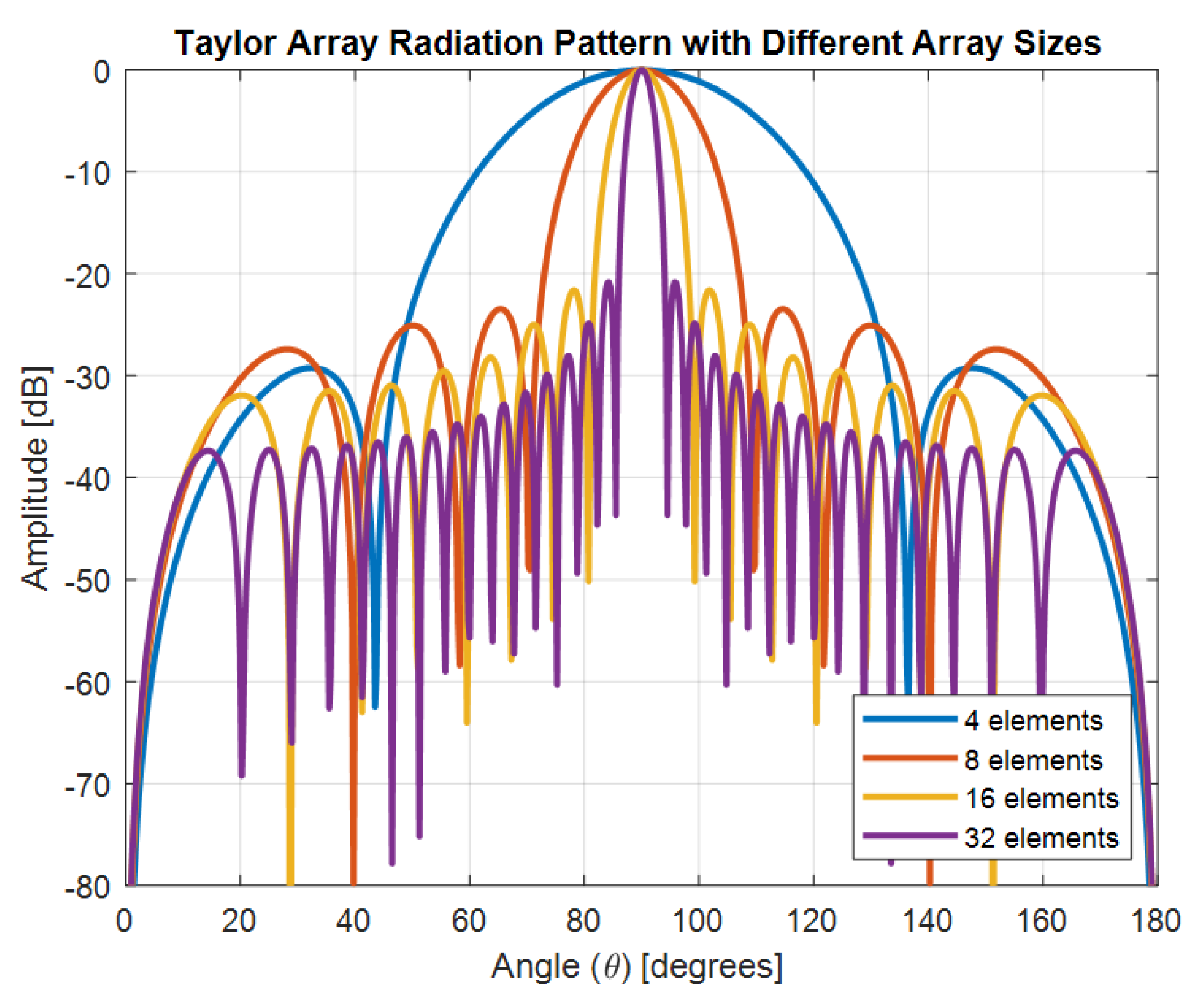
Thus, increasing the number of elements in the array results in a narrower beam and better angular resolution, but it also requires optimal element spacing to avoid the formation of grating lobes. If the element spacing, d, exceeds $\lambda /2$, unwanted side lobes, or grating lobes, may appear, leading to detection errors. To mitigate these effects, windowing functions such as Taylor, Chebyshev, or Hamming windows are applied to reduce side lobes, optimizing radar performance without significantly increasing the main beam width [26,27]. Among these, Taylor-series expansion is favored in this work due to its analytical tractability and ability to produce physically interpretable excitation profiles with controlled sidelobe behavior. Unlike Chebyshev- or Fourier-based designs, Taylor excitation enables the smooth tapering of the amplitude distribution, which integrates naturally with neural network optimization and facilitates convergence. This balance between simplicity, control, and compatibility with data-driven tuning makes Taylor series a strong candidate for hybrid synthesis frameworks.

Phased-array radars enable electronic beam steering, where the beam can be directed in any direction by electronically adjusting the phase of each array element. This allows for faster scanning compared to traditional mechanical antenna radars, as well as real-time adaptability to track multiple targets simultaneously, which is essential for modern radar systems used in defense, airborne surveillance, weather radars, and autonomous vehicles. By adjusting the phases, $\beta$, of the array elements, the radar can track multiple targets, perform frequency hopping across different angles, and provide real-time information on the position and velocity of targets [28].

Phased array radars are used in critical applications where speed and accuracy are essential [29,30,31]. For example, in missile defense, phased array radars such as the AN/SPY-1 enable the real-time detection and tracking of missiles. Similarly, in airborne radar systems, AESA (active electronically scanned array) radars provide comprehensive surveillance of airspace, enabling precise flight path control and the better detection of stealth targets. In meteorology, these radars allow for the detailed monitoring of weather phenomena, such as storms and precipitation, with high spatial resolution and the ability to scan large areas quickly.

Phased-array radars offer advanced capabilities in electronic beam steering and multi-target detection, enabling them to be used in a wide range of complex applications. The precise control of the beam, enabled by the array factor, and the ability to adapt to dynamic tracking needs make phased array radars an essential technology in modern defense, airborne surveillance, and intelligent transportation systems.

Figure 1 illustrates the structure of a smart antenna, which consists of an array of antennas, including both analog and digital low noise amplifiers (LNAs), a high-power amplifier (HPA), a power amplifier (PA), an analog-to-digital Converter (ADC), a digital-to-analog converter (DAC), a local oscillator (LO) for baseband transmission (Tx) and reception (Rx), and the weights for antenna array synthesis. The antenna array synthesis involves adjusting the weights applied to each antenna element to optimize the overall radiation pattern and performance of the system for various communication or sensing applications, based on the architecture proposed by Prof. A. Manikas [32].

3. The Taylor Method

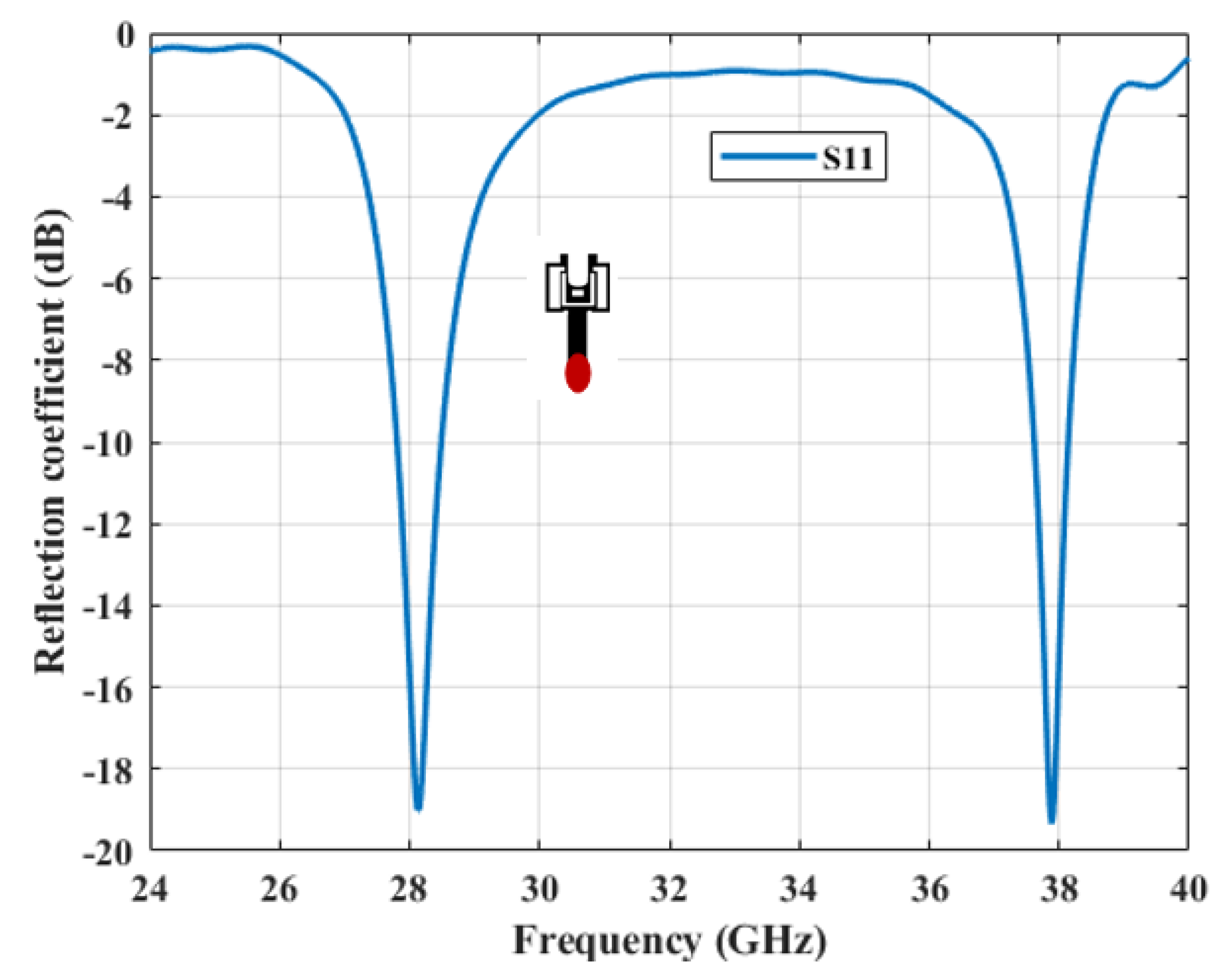
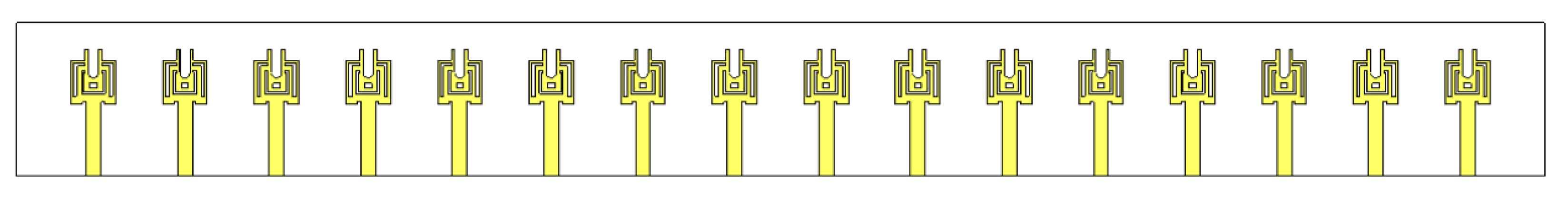
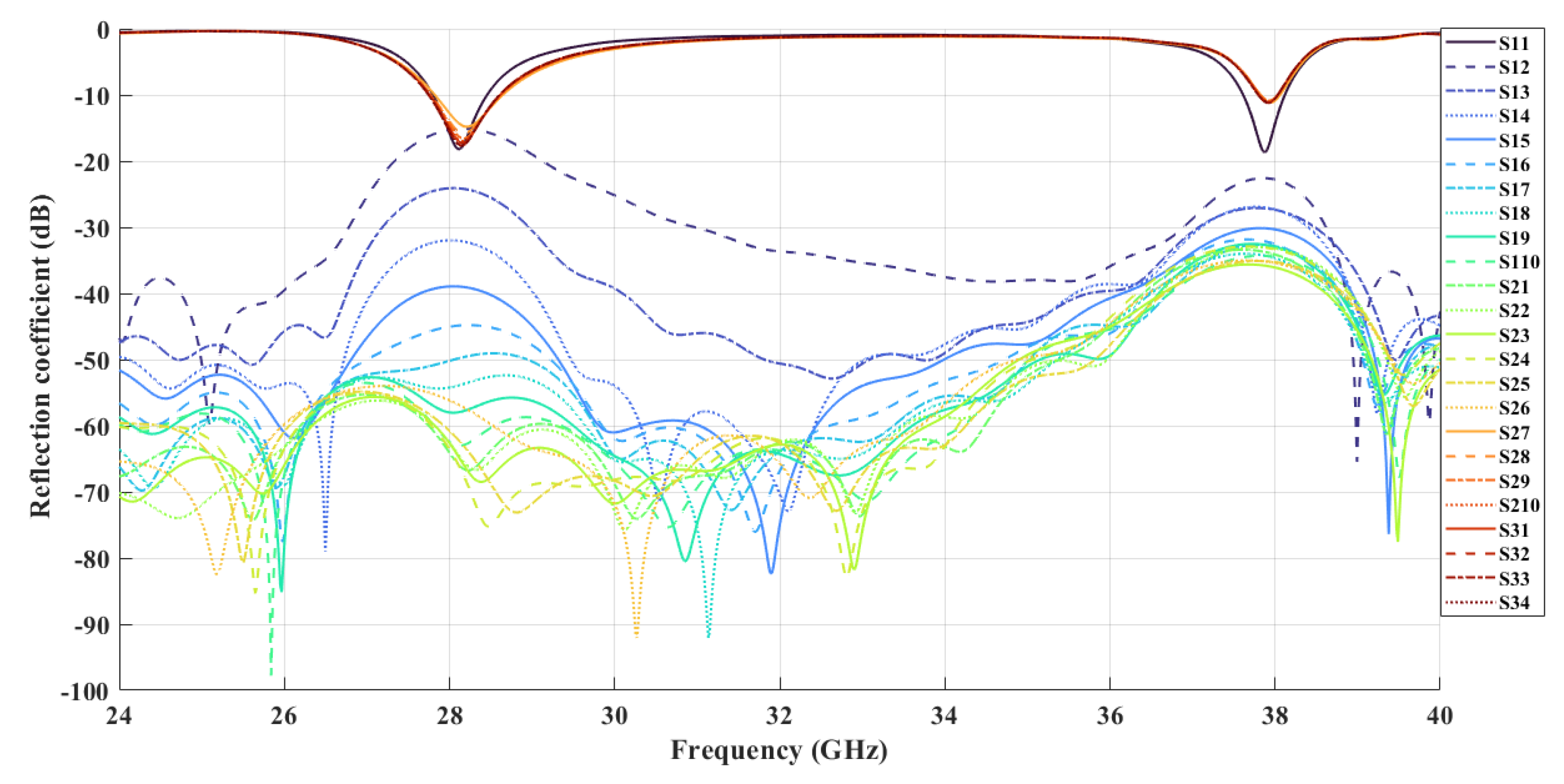
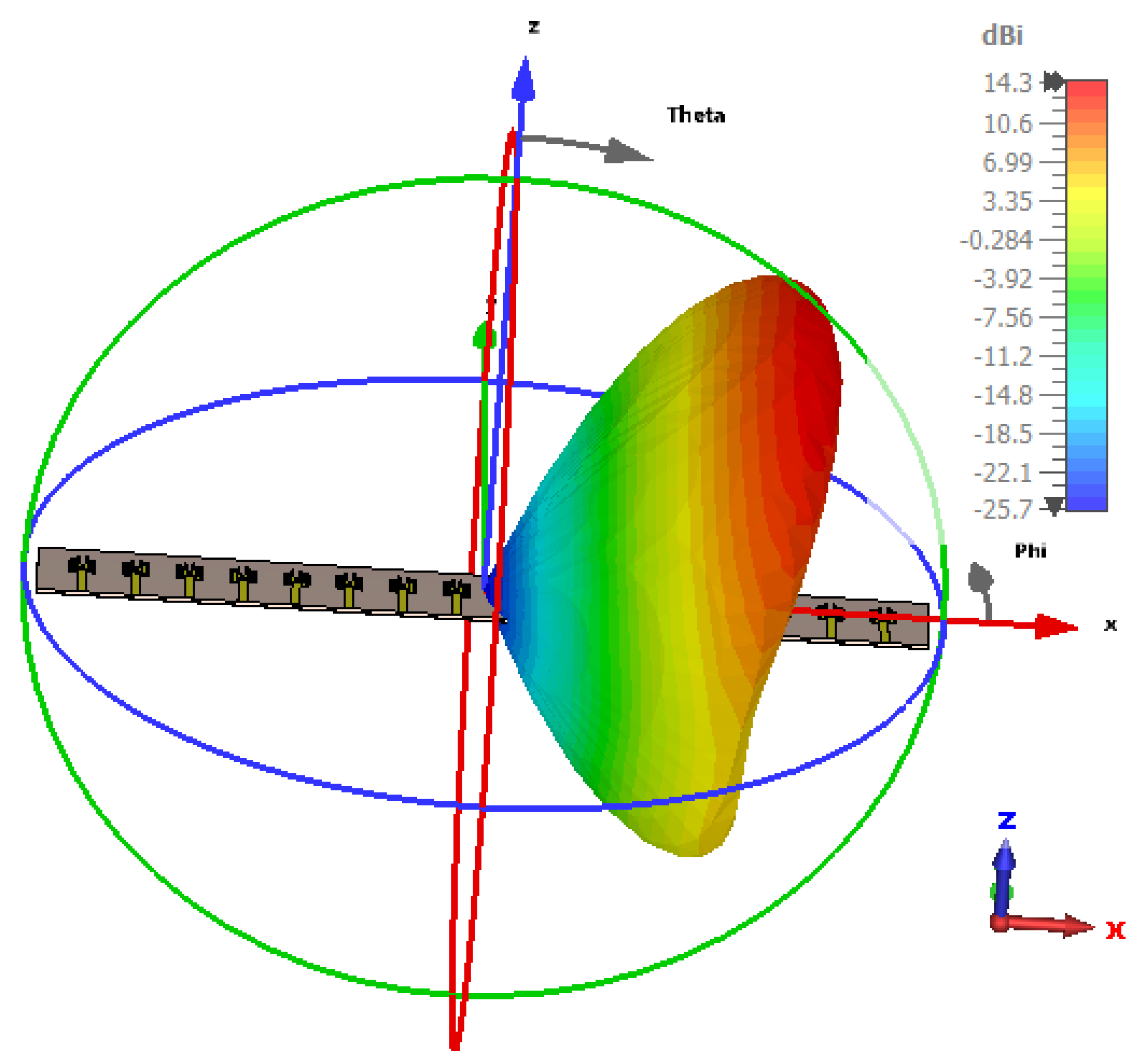
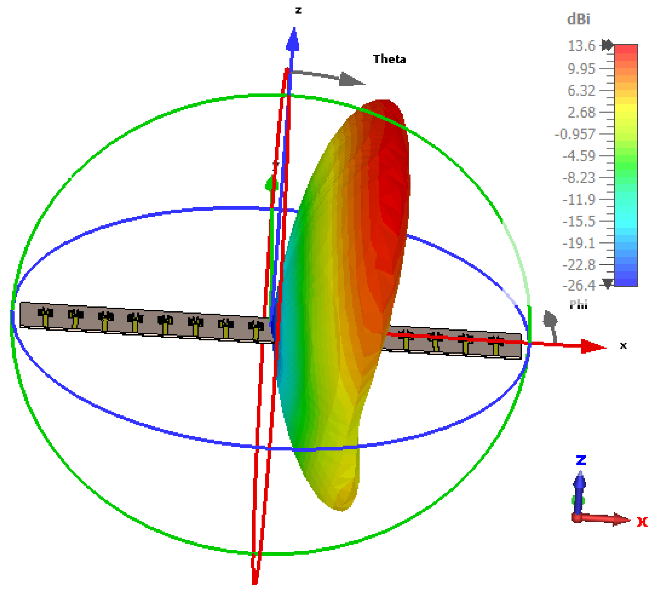
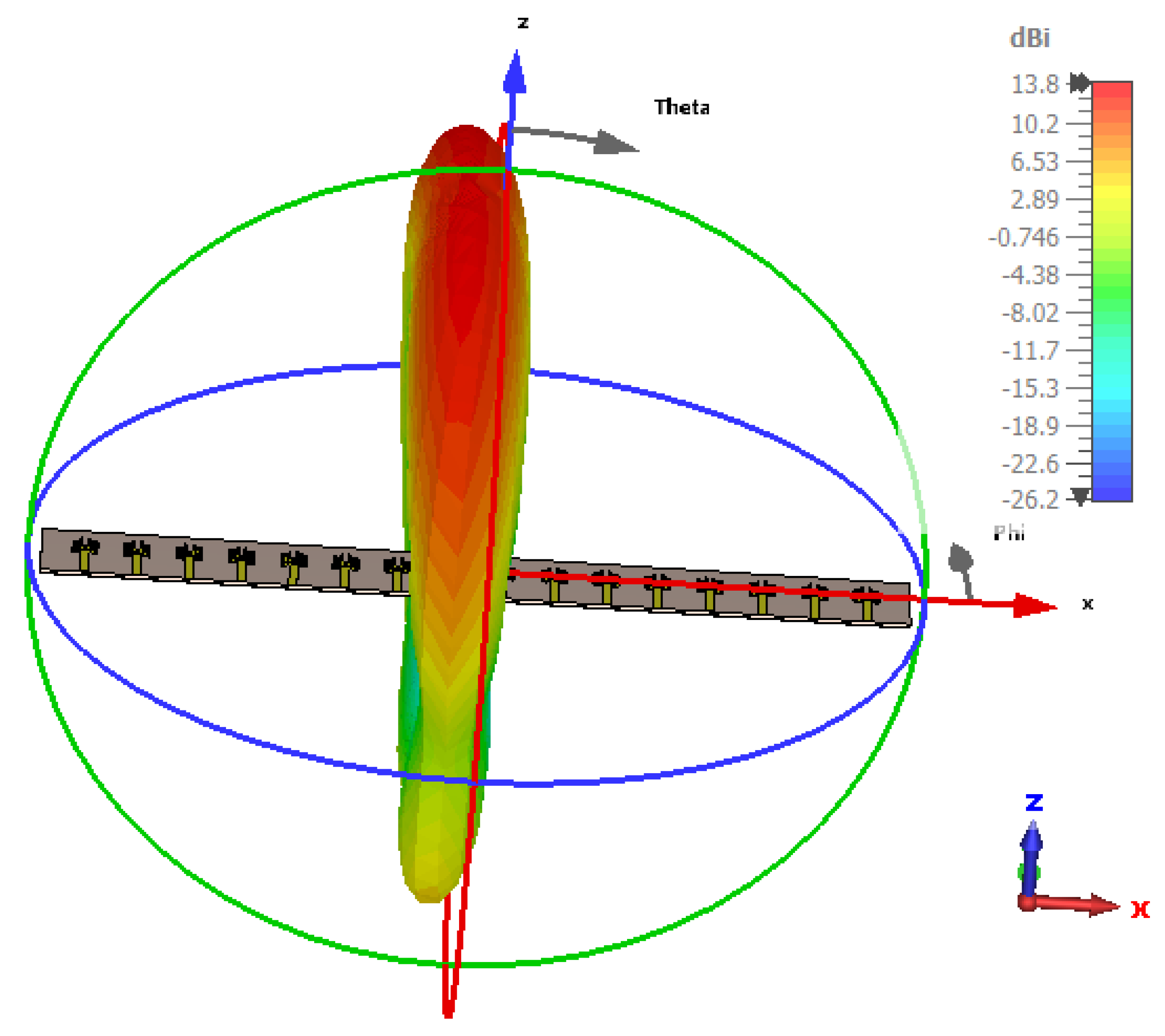
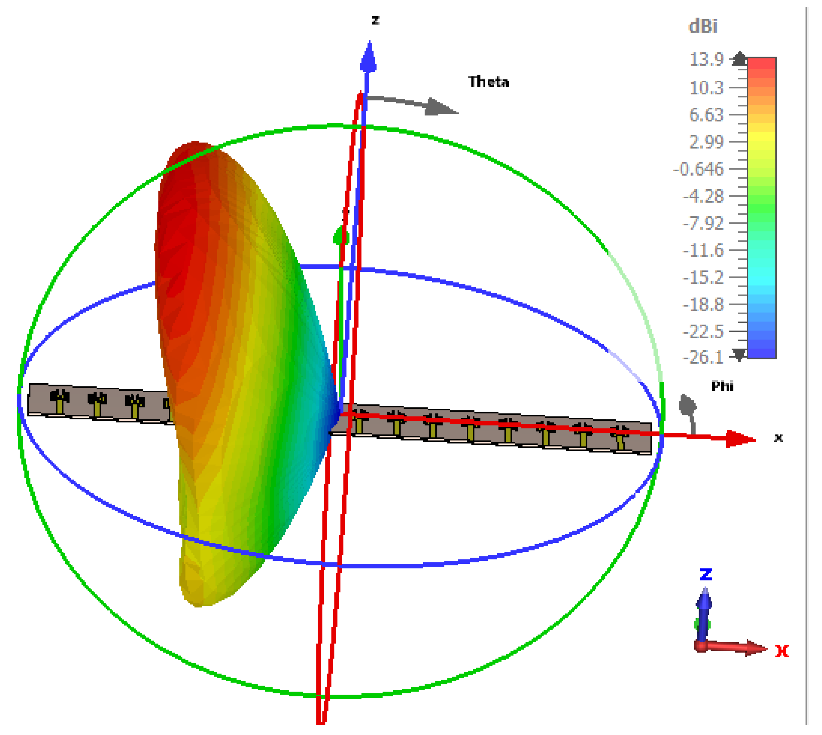
The simulated antenna consists of 16 identical microstrip patch elements arranged in a uniform linear array with $\lambda /2$ spacing. This structure serves as the physical basis for the optimization framework and simulation results presented in Figure 2, Figure 3, Figure 4 and Figure 5. The Taylor method is a classical technique used in antenna array design to control how energy is distributed across the radiation pattern. It enables designers to fine-tune parameters such as beamwidth and sidelobe level by adjusting excitation amplitudes across the array elements using a mathematical series expansion. When a precise expression of the electromagnetic field is not easily available, Taylor expansion allows engineers to locally approximate the field distribution and apply optimized amplitude weights to shape the desired beam [25,33,34,35].

Using spherical coordinates $(r,\theta ,\varphi )$, where r represents the radial distance from the observation point, $\theta$ represents the azimuthal angle, and $\varphi$ represents the elevation angle, the Taylor method can be extended to approximate the spatial distribution of the electromagnetic field as follows [36,37]:

$$E(r,\theta ,\varphi )\approx E(r_0,{\theta }_0,{\varphi }_0)+{\left.{\displaystyle \frac{\partial E}{\partial r}}\right|}_{(r_0,{\theta }_0,{\varphi }_0)}(r-r_0)+{\left.{\displaystyle \frac{\partial E}{\partial \theta }}\right|}_{(r_0,{\theta }_0,{\varphi }_0)}(\theta -{\theta }_0)+{\left.{\displaystyle \frac{\partial E}{\partial \varphi }}\right|}_{(r_0,{\theta }_0,{\varphi }_0)}(\varphi -{\varphi }_0)$$

(5)

In this expression, the following applies:

• $E(r,\theta ,\varphi )$ represents the spatial distribution of the electromagnetic field of the antenna array.
• $(r_0,{\theta }_0,{\varphi }_0)$ is the reference point around which the Taylor series is developed.
• ${\displaystyle \frac{\partial E}{\partial r}}$, ${\displaystyle \frac{\partial E}{\partial \theta }}$, and ${\displaystyle \frac{\partial E}{\partial \varphi }}$ are the partial derivatives of E with respect to r, $\theta$, and $\varphi$ respectively, evaluated at the reference point $(r_0,{\theta }_0,{\varphi }_0)$.

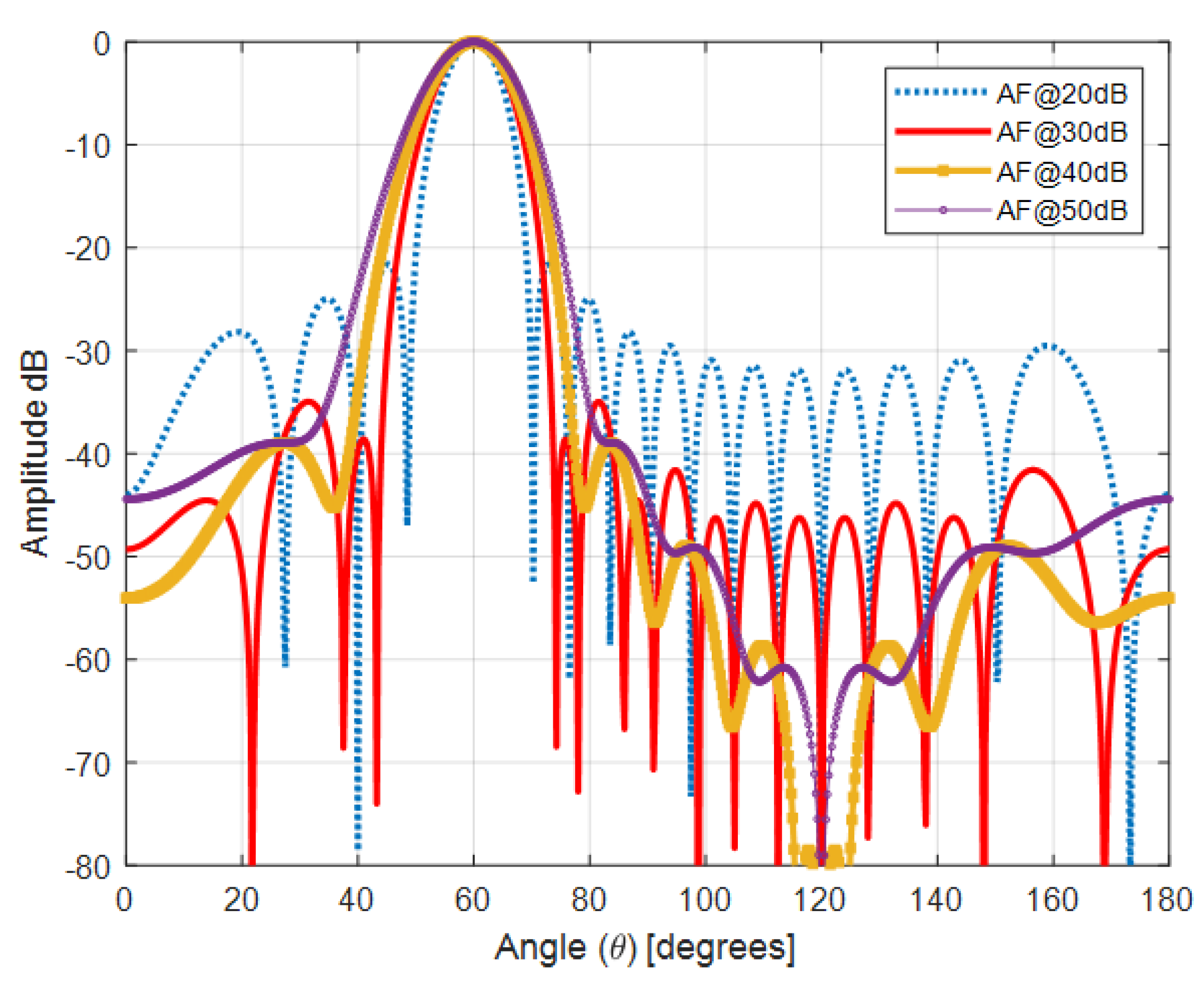
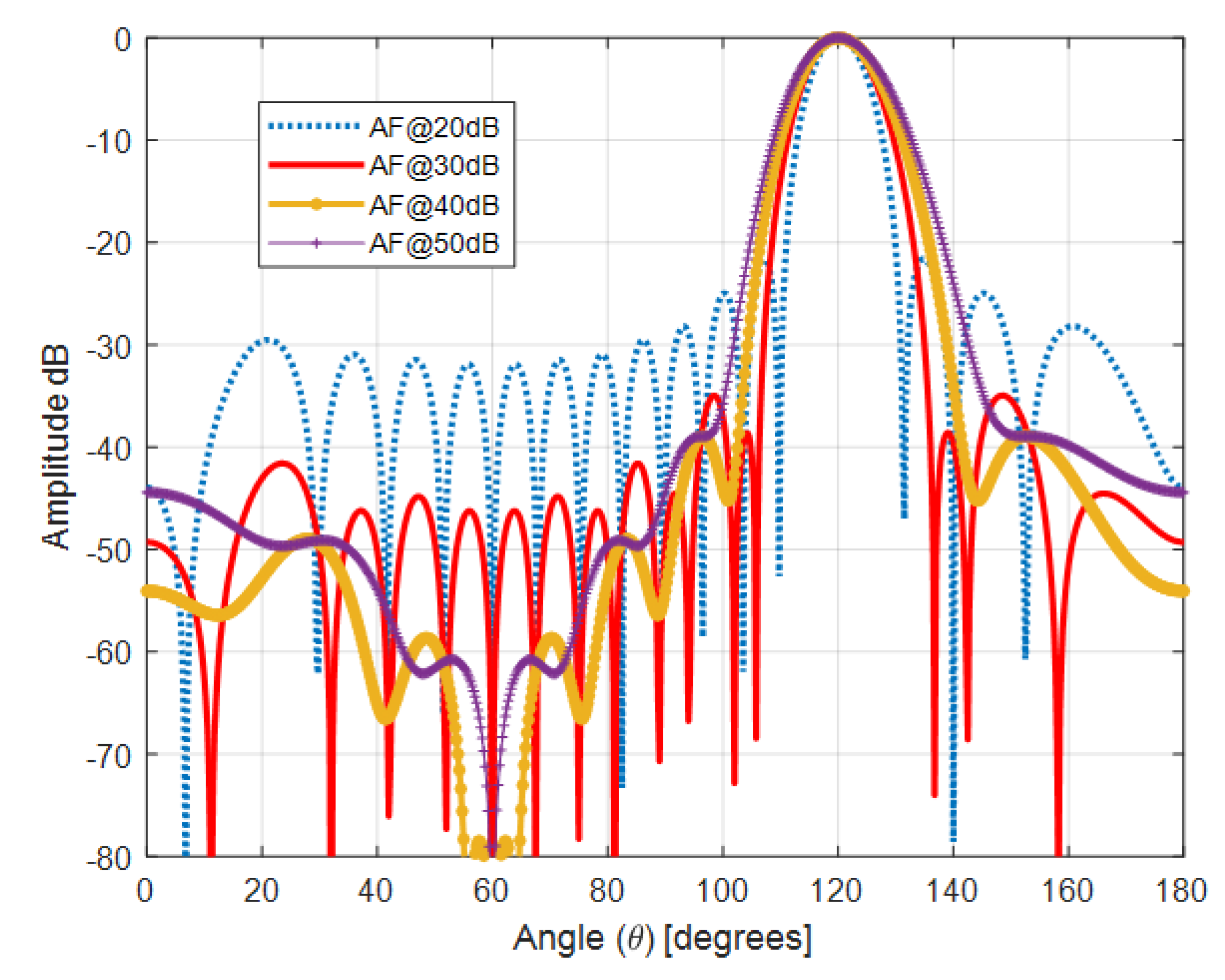
The Taylor method is utilized in antenna design to dictate the amplitude attenuation of elements within an antenna array, often characterized by a single parameter such as the main lobe width. This amplitude attenuation, when applied to the array elements, directly impacts the array factor, a mathematical function delineating each array element’s contribution to the overall radiation pattern formation. Thus, employing the Taylor method to ascertain the amplitude of array elements directly influences the array factor and subsequently the comprehensive radiation pattern of the antenna array [38,39,40]. Through parameter adjustments in the Taylor method, like modifying the main lobe width, one can manipulate the amplitude of the array factor, enabling precise control and optimization of the antenna array’s radiation pattern to align with specific requirements. This Algorithm 1 outlines the steps to synthesize a Taylor–Kaiser antenna array. It starts by choosing the appropriate window and calculating coefficients based on the given specifications. Then, for each antenna element, it calculates the weight and position. If the performance is satisfactory, it finalizes the design; otherwise, it adjusts the parameters to improve performance.

Algorithm 1 Synthesize Taylor–Kaiser antenna array.

1: function Synthesize Antenna(specs)   2:     Step 0: Initialize Parameters   3:          Define the number of elements N and the desired sidelobe level (SLL).   4:          Set the beamwidth and aperture size according to specs.   5:     Step 1: Select Window Function   6:          Choose the appropriate window (Taylor or Kaiser) based on SLL and beamwidth.   7:     Step 2: Calculate Array Coefficients   8:          Compute the excitation coefficients for each element using the selected window.   9:     Step 3: Compute Element Weights and Positions 10:     for $i=1$ to N do 11:         Calculate weight $\mathrm{Weight}\left[i\right]$ = WindowFunction($i,N$). 12:         Calculate element position $\mathrm{Position}\left[i\right]$ = $d\times (i-(N+1)/2)$, where d is the element spacing. 13:     end for 14:     Step 4: Evaluate Performance 15:     Compute the radiation pattern and evaluate sidelobe levels, beamwidth, and directivity. 16:     Step 5: Adjust and Finalize 17:     if Performance is satisfactory then 18:         Finalize the array design and export the parameters. 19:     else 20:         Adjust window parameters or element spacing and repeat from Step 2. 21:     end if 22: end function

This Taylor series can be truncated after the first order if a linear approximation is sufficient for the spatial distribution of the electromagnetic field around the reference point.

The amplitude distribution for the Taylor one-parameter distribution is given by the following:

$$w_n\left(\alpha \right)={\displaystyle \frac{J_0\left(\alpha \sqrt{1-{\rho }^2}\right)}{J_0\left(\alpha \right)}}$$

(6)

where the following applies:

• $w_n\left(\alpha \right)$ is the amplitude weighting coefficient for the n-th element of the array.
• $J_0$ is the zeroth-order Bessel function of the first kind.
• $\alpha$ is the design parameter that controls the characteristics of the radiation pattern.
• $\rho ={\displaystyle \frac{2\pi d}{\lambda }}sin\left(\theta \right)$ is the normalized distance between array elements, where

  -

  d is the spacing between elements;

  -

  $\lambda$ is the wavelength;

  -

  $\theta$ is the angle of radiation.

The Bessel function of the first kind of order zero, $J_0\left(x\right)$, is defined by the infinite series:

$$J_0\left(x\right)=\sum _{k=0}^{\infty }{\displaystyle \frac{{(-1)}^k}{{(k!)}^2}}{\left({\displaystyle \frac{x}{2}}\right)}^{2k}$$

(7)

It satisfies the recurrence relation:

$$J_0\left(x\right)={\displaystyle \frac{2}{x}}{J}_1\left(x\right)-J_{-1}\left(x\right)$$

(8)

and its asymptotic behavior for large x is approximated by

$$J_0\left(x\right)\approx \sqrt{{\displaystyle \frac{2}{\pi x}}}cos\left(x-{\displaystyle \frac{\pi }{4}}\right)$$

(9)

This function frequently appears in applications such as wave propagation in cylindrical waveguides, heat conduction in cylindrical coordinates, and vibration analysis in cylindrical structures.

3.1. Synthesizing Antenna Arrays Using Taylor One-Parameter Distribution

Synthesizing antenna arrays using the Taylor one-parameter distribution involves defining requirements such as radiation pattern and beamwidth, selecting array geometry and element patterns, applying the Taylor distribution to determine element amplitude tapering, calculating the array factor to describe pattern formation, optimizing parameters through iterative refinement, and validating the design via simulation or testing. This process enables the creation of antenna arrays tailored to specific needs, whether for beamforming, direction finding, or other applications [41,42,43,44].

3.1.1. Define Radiation Pattern Requirements

In the first step of antenna synthesis, it is essential to define how the antenna should radiate. This includes specifying the width of the main beam (which affects angular coverage), the acceptable levels of sidelobes (to reduce interference), and the placement of nulls (to suppress unwanted directions). These criteria guide the selection of parameters in the Taylor distribution, ensuring that the final design meets application-specific performance needs, such as high resolution in radar or reduced interference in wireless systems [45,46]. The main lobe width defines the angular spread of the primary radiation direction, influencing the antenna’s coverage area and directionality. Meanwhile, the side lobe level indicates the level of radiation in directions other than the main lobe, with lower levels indicating better rejection of unwanted radiation. Additionally, the placement of nulls in the radiation pattern can be strategically determined to minimize interference or steer the beam away from sources of noise or interference. These requirements serve as guiding principles for selecting design parameters, such as $\alpha$ in the Taylor one-parameter distribution, shaping the antenna array’s behavior to meet specific performance criteria essential for its intended application.

• Determine the desired characteristics of the radiation pattern, such as the side lobe level, the main lobe width, and null placement.
• These requirements will guide the selection of the design parameter $\alpha$.

3.1.2. Select Design Parameter $\alpha$

The design parameter $\alpha$ in antenna array synthesis using the Taylor one-parameter distribution represents the main lobe width or beamwidth, crucial for controlling the radiation pattern’s directivity and sidelobe levels.

• The design parameter $\alpha$ determines the overall shape of the amplitude distribution.
• Choose $\alpha$ based on the desired trade-off between the side lobe level and the main lobe width.
• Higher values of $\alpha$ result in lower side lobes but wider main lobes, and vice versa.

3.1.3. Calculate Amplitude Weights

The amplitude weights $w_n$ for an antenna array using the Taylor one-parameter distribution are calculated as follows:

• Use the formula $w_n\left(\alpha \right)={\displaystyle \frac{J_0\left(\alpha \sqrt{1-{\rho }^2}\right)}{J_0\left(\alpha \right)}}$ to calculate the amplitude weighting coefficients for each element of the array.
• $\rho$ depends on the array geometry and the angle of radiation.

3.1.4. Apply Amplitude Weights

The amplitude weights $w_n$ are applied to the elements of an antenna array by multiplying each element’s magnitude by its corresponding weight. The weighted amplitude $w_n$ of the nth element is calculated as follows:

• Apply the calculated amplitude weighting coefficients as the weights for the elements of the antenna array.
• These weights determine the relative strength of each element and thus shape the radiation pattern.

3.2. Example 1

Figure 2 illustrates the synthesis of antenna weights for varying lobe widths and array sizes, demonstrating how these factors influence the radiation pattern. By adjusting the antenna weights, it is possible to control the main lobe’s width, affecting both angular resolution and directivity. Additionally, increasing the array size sharpens the beam, reduces side lobes, and enhances gain in the primary direction. This optimization process aims to shape the radiation pattern to minimize interference and maximize system performance.

In Example 1, the radiation patterns of antenna arrays are generated and analyzed using the Taylor method for different array sizes (4, 8, 16, and 32 elements). The taylor1p function is used to calculate the weights of the array, considering a side-lobe level of 20 dB and a half-wavelength element spacing. The gain1d function then computes the array gain at 720 angles. The radiation patterns (gain versus angle) are plotted for each array configuration, with thickened curves for better visibility using the LineWidth property. Additionally, the weights are converted into magnitude and phase values, which are displayed in degrees. The results are presented both numerically (magnitude and phase) and graphically in dB, showcasing how increasing the number of array elements reduces sidelobes and narrows the main lobe. This demonstrates the impact of Taylor’s array synthesis method on antenna performance.

3.3. Example 2

To achieve the specified side lobe levels (−20 dB, −30 dB, −40 dB, and −50 dB), amplitude tapering among the elements is optimized using Taylor distributions. This optimization ensures that the radiation pattern meets the desired sidelobe levels. The main lobe width can be adjusted accordingly during the optimization process to meet any specific requirements. Finally, the array factor representing the radiation pattern is computed, followed by simulation and iterative optimization using MATLAB R2023a until meeting the specified design criteria [47].

Figure 3 shows the Taylor antenna array with a Kaiser window, where the array size is $N=16$, and the inter-element spacing is $d={\displaystyle \frac{\lambda }{2}}$. This configuration operates at an angle of ${60}^{°}$, demonstrating the radiation pattern at this specific angle. Figure 4 presents a similar Taylor antenna array with the same parameters ($N=16$, $d={\displaystyle \frac{\lambda }{2}}$), but the array operates at ${90}^{°}$. Finally, Figure 5 illustrates the Taylor antenna array with a Kaiser window under the same conditions, but operating at ${120}^{°}$. These figures highlight how the antenna’s radiation pattern varies with different operating angles while maintaining the same array size and element spacing.

4. Validation Using CST Microwave Studio for 5G Antenna Arrays

4.1. Antenna Design

The basic structure envisaged for validation is a dual-band rectangular microstrip patch antenna fabricated on a Rogers RT4003C substrate. It exhibits two resonances at 28.14 GHz and 37.88 GHz, tailored for 5G applications. The substrate features a thickness of 0.41 mm, a relative permittivity of ${\epsilon }_r=3.55$, and a low loss tangent of 0.0027. The patch is fed via a 50 $\Omega$ microstrip line to ensure proper impedance matching. Dual-band operation is achieved through slot insertion and careful tuning of the patch geometry. All geometric parameters—including length, width, slot configuration, and feed position—were first derived analytically and then refined through full-wave CST simulations.

Millimeter-wave (mm-wave) frequency bands have attracted considerable attention in wireless communications, particularly for 5G networks, due to their wide spectral bandwidth and ability to support exceptionally high data rates. To harness these frequency bands effectively, a meticulous antenna design process is essential, with the selection of substrate material playing a pivotal role. Parameters such as thickness, relative permittivity, and loss tangent directly impact the antenna’s electromagnetic performance, influencing radiation efficiency, impedance matching, and dielectric losses. In this section, we will design and simulate antenna arrays to validate our method using CST Microwave Studio.

We also present the design and optimization of a dual-band antenna operating at the critical 5G frequencies of 28 GHz and 38 GHz, specifically tailored to next-generation communication systems. The proposed antenna is fabricated using the Rogers RT4003C substrate, selected for its excellent electromagnetic properties, which are characterized by the following:

• Thickness: 0.41 mm.
• Relative permittivity: ${\epsilon }_r=3.55$.
• Loss tangent: $tan\delta =0.0027$.

The antenna is fed via a 50 $\Omega$ microstrip transmission line to ensure optimal impedance matching with high-frequency circuitry. Its structural design features a rectangular patch geometry with a radiating element of width W and length L, carefully determined using classical analytical models for microstrip patch antennas. The slot dimensions were empirically adjusted to support the dual-band response and ensure proper impedance matching.

Geometric parameter optimization aimed at minimizing reflection losses, enhancing radiation efficiency, and meeting the stringent requirements of mm-Wave communications. The final antenna dimensions are summarized in Figure 6 and

Table 2. Geometric parameters of the antenna.

Parameter	Value (mm)	Parameter	Value (mm)
WS	4.5	Wb	0.4
LS	4.5	Lb	0.3
Lp	2.6	LC2	1.8
Lu	0.65	L3	1.4
Wu	0.2	WK	0.8
Le	0.2	Lt	0.2
We	0.44	Wt	0.2
LC1	1.1	Lf	4.34
WC1	1.4	Wf	0.86
R	0.3

, illustrating the necessary design refinements for stable operation at the target frequencies.

The patch width W is calculated using the following equation:

$$W={\displaystyle \frac{c}{2f_c\sqrt{({\epsilon }_r+1)/2}}}$$

(10)

The central frequency, $f_c$, and the effective permittivity, ${\epsilon }_{eff}$, are crucial in determining the microstrip patch antenna dimensions. The effective permittivity, accounting for the dielectric substrate’s influence, is given by the following:

$${\epsilon }_{eff}={\displaystyle \frac{{\epsilon }_r+1}{2}}+{\displaystyle \frac{{\epsilon }_r-1}{2}}{\left(1+12{\displaystyle \frac{h}{W}}\right)}^{-0.5}$$

(11)

where h is the substrate thickness.

The extended incremental length, $\Delta L$, caused by fringing fields, is approximated as follows:

$$\Delta L=0.412h{\displaystyle \frac{({\epsilon }_{eff}+0.3)(W/h+0.264)}{({\epsilon }_{eff}-0.258)(W/h+0.8)}}$$

(12)

The effective length $L_{eff}$ is calculated as follows:

$$L_{eff}={\displaystyle \frac{c}{2f_c\sqrt{{\epsilon }_{eff}}}}$$

(13)

Finally, the actual physical length L, accounting for fringing effects, is determined by the following:

$$L=L_{eff}-2\Delta L$$

(14)

where c is the speed of light in free space ($3\times {10}^8$ m/s), and $f_c$ is the resonant frequency.

This detailed design methodology ensures that the proposed antenna meets the stringent performance requirements of 5G millimeter-wave communications while achieving optimal impedance matching and enhanced radiation efficiency. Equations (10)–(15) present standard design formulas for microstrip patch antennas. They are included here for completeness and clarity and are derived from the classical reference [25].

To enhance the analytical understanding of the antenna’s dual-band behavior, an equivalent circuit model (ECM) is proposed, as shown in Figure 7. The ECM consists of two parallel RLC resonators, each representing one of the antenna’s resonant frequencies at 28.14 GHz and 37.88 GHz. These branches are connected to a 50 $\Omega$ transmission line that models the microstrip feed. Each RLC cell captures the resonant characteristics, impedance response, and loss mechanisms of its respective frequency band. This circuit-level abstraction provides an analytical perspective on the impedance matching and coupling effects observed in the electromagnetic simulations and can serve as a useful tool for future parametric tuning and rapid prototyping. Although a detailed parameter extraction is outside the scope of this work, the conceptual ECM reinforces the physical interpretation of the antenna design. Such equivalent circuit models have been widely adopted in the literature to interpret the impedance behavior and mode separation in dual-band or multi-band antennas, especially in the millimeter-wave range [48,49].

The analysis of the results presented in Figure 8 highlights the dual-band behavior of the proposed antenna. It shows distinct resonances at 28.14 GHz and 37.88 GHz, with respective reflection coefficients of S₁₁ = −19 dB and S₁₁ = −19.33 dB. These values indicate optimal impedance matching, significantly reducing reflection losses and ensuring efficient signal transmission in the two targeted frequency bands.

Figure 9, which represents the antenna’s directivity, highlights the antenna’s ability to focus its radiation in a specific direction. The directivity of the antenna is 5.98 dBi, indicating that the antenna emits in a narrow beam, concentrating energy in a particular area. This high directivity is essential for applications like point-to-point communications and radar systems. Conversely, low directivity would indicate broader coverage but less targeted radiation. Figure 10 shows the antenna’s gain, which measures the antenna’s efficiency in transmitting or receiving signals in a given direction compared to an isotropic antenna. The gain of the antenna is 4.29 dBi, meaning the antenna is quite efficient at focusing energy in a specific direction. A high gain enhances the range and performance in applications for which signal focus is crucial, such as long-distance communication systems, satellites, and radar. Together, these two parameters (directivity of 5.98 dBi and gain of 4.29 dBi) characterize the antenna’s efficiency and performance in various use cases.

The 3D radiation pattern of the antenna, presented in Figure 11, provides valuable insights into the antenna’s performance at two distinct frequencies: (a) at 28.14 GHz and (b) at 37.88 GHz.

(a) At 28.14 GHz: The radiation pattern at this frequency shows a specific distribution of the radiated energy, with the main lobe directed at a particular angle, indicating the primary direction of maximum radiation. The pattern might exhibit a relatively narrow beamwidth, which suggests that the antenna is highly directional at this frequency, focusing its energy towards a specific region in space. Side lobes and back lobes might also appear, indicating minor radiation in directions other than the main beam. The low sidelobe levels typically indicate minimal unwanted radiation, contributing to higher efficiency in the desired direction.

(b) At 37.88 GHz: At this higher frequency, the antenna’s radiation pattern could differ significantly, reflecting a change in its directional properties. The main lobe might shift in angle or broaden, depending on the antenna design and its impedance matching at this frequency. Higher frequencies typically result in a narrower beamwidth, but the antenna might also demonstrate a more complex radiation pattern due to factors like frequency-dependent impedance mismatch or interference effects. The side lobes may also appear differently, and the overall pattern might show reduced efficiency in certain directions due to different propagation characteristics at this higher frequency.

In both cases, the patterns highlight the dual-band performance of the antenna, which is crucial for applications requiring high efficiency in multiple frequency bands. The optimal radiation patterns at 28.14 GHz and 37.88 GHz ensure that the antenna can be effectively used in these bands, minimizing reflection losses and maximizing signal transmission in their respective regions.

4.2. 16-Element MIMO Antenna Array

The MIMO system under investigation comprises 16 antennas aligned in the same direction and arranged parallel to each other, with an inter-element spacing of $\lambda /2$, as shown in Figure 12. This configuration has been carefully designed to maximize network directivity while minimizing mutual coupling between radiating elements, ensuring efficient signal transmission in millimeter-wave frequency bands. Each patch element has a width of $W=2.6$ mm and a length of $L=2.6$ mm and is designed on a substrate with a thickness of $h=0.41$ mm. The elements are uniformly spaced by $\lambda /2$, resulting in a total array length of approximately 89.4 mm. The results presented in Figure 13 highlight the stability of mutual coupling across the entire operational frequency band. Specifically, the electromagnetic performance assessment shows that the maximum mutual coupling between antennas remains below −15 dB, indicating excellent isolation among the array elements. Such a high degree of isolation is essential for preserving radiation efficiency, as it reduces interference and mitigates losses caused by unwanted electromagnetic interactions. This characteristic is crucial for optimizing MIMO system performance, enabling enhanced spatial multiplexing and higher data transmission rates, particularly in millimeter-wave communication systems.

The Figure 13 shows the S-parameters of the antenna, which are crucial for assessing its reflection and transmission characteristics. S₁₁ represents the reflection coefficient, indicating how much signal is reflected back into the antenna; lower values (typically below −10 dB) suggest good impedance matching and minimal reflection losses. S₂₁ indicates the forward transmission efficiency, with higher values reflecting better signal transmission. S₁₂, the reverse transmission coefficient, should ideally be low to minimize back reflections, while S₂₂, the reflection coefficient at the output port, provides insight into the matching at the output. Overall, low reflection coefficients (S₁₁ and S₂₂) and high transmission coefficients (S₂₁) indicate optimal antenna performance, ensuring efficient signal transmission with minimal losses across the operating frequencies.

Figure 14, Figure 15, Figure 16, Figure 17, Figure 18, Figure 19, Figure 20, Figure 21, Figure 22, Figure 23, Figure 24 and Figure 25 show the radiation patterns of the antenna at various angles, ranging from 25° to 135°. At lower angles such as 25° and 35°, the radiation pattern is more concentrated, with the main lobe pointing in a specific direction, indicating a narrower beamwidth. As the angle increases to 45° and 55°, the main lobe begins to widen, indicating an expansion of the radiation coverage. This trend continues through angles of 65°, 75°, and 85°, when the antenna starts to radiate more broadly, providing wider coverage. At higher angles, such as 95° to 135°, the radiation pattern continues to spread, and the energy is directed over a larger area. The main lobe shifts progressively, and the side lobes also change in intensity, reflecting how the antenna adapts its radiation characteristics across different angular orientations. This behavior illustrates the antenna’s ability to provide directional or omnidirectional radiation, depending on the required application, and it emphasizes the flexibility of the antenna design in accommodating a wide range of angular orientations for optimal signal distribution. Figure 26 presents the radiation pattern of 16 antennas synthesized using the Taylor method with different amplitude synthesis levels of −20 dB, −30 dB, −40 dB, and −50 dB, along with uniform excitation.

5. Neural Networks for Synthesis and Optimization of Antenna Arrays

Artificial neural networks (ANNs) provide a flexible and powerful framework for improving antenna array design. These models are capable of learning complex, nonlinear relationships between the excitation parameters of antenna elements and the resulting radiation pattern. Once trained, ANNs can quickly predict optimal excitation weights to achieve desired performance metrics such as minimized sidelobe levels or enhanced beam directivity. This is particularly useful in adaptive antenna systems, where fast real-time adjustments are needed to respond to changing environments, such as in mobile communication, radar, or satellite applications. By training on large datasets, ANNs can optimize parameters such as directivity, sidelobe levels, and the overall adaptability of antenna arrays. This capability enables them to deliver superior results compared to traditional optimization techniques.

In particular, neural networks can significantly improve the performance of antenna arrays by reducing sidelobes, enhancing the main lobe, and optimizing array configurations to achieve specific radiation patterns. They are capable of managing multiple constraints simultaneously, such as power distribution, array size, and performance under various environmental conditions. This makes ANNs particularly useful in designing adaptive and reconfigurable antenna systems for advanced communication systems, radar, and smart antennas.

In comparison to conventional numerical methods like Taguchi, Sequential Quadratic Programming (SQP), Dolph–Chebyshev, and Particle Swarm Optimization (PSO), neural networks offer faster convergence and are more effective at dealing with the complexity of large parameter spaces. These traditional methods often require iterative processes that can be computationally expensive and time-consuming. However, ANNs, once trained, can generate solutions quickly and with high accuracy.

The dataset used in this context is based on numerical algorithms and synthesis techniques, including Taguchi, SQP, Dolph-Chebyshev, and PSO. These methods are well established in antenna array design for optimizing radiation patterns, but in this paper, the focus is specifically on the synthesis of antenna arrays using the Taylor method. The Taylor method allows for the generation of optimal phase distributions and array element positions, leading to highly efficient antenna designs. By integrating this method with the power of neural networks, this approach aims to further enhance the synthesis process and improve overall array performance.

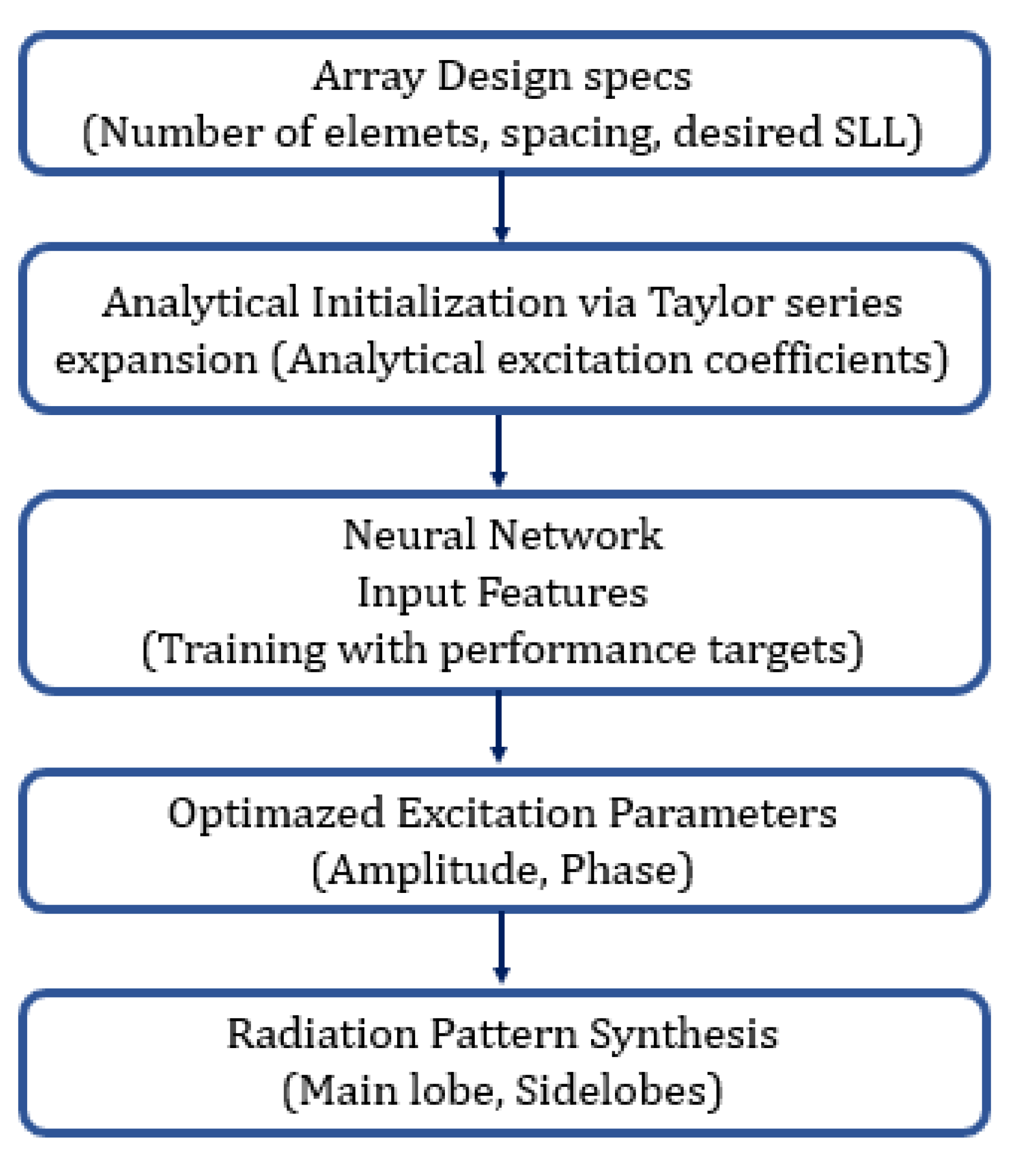
To bridge the analytical synthesis and neural optimization components of our approach, a visual representation of the workflow is introduced below.

To facilitate a clearer understanding of the proposed hybrid approach, Figure 27 presents a flowchart illustrating the interaction between the Taylor series expansion and the neural network. This schematic outlines the sequential process beginning with array design specifications, followed by the analytical initialization of excitation coefficients via the Taylor method. These coefficients are then used as input features for the neural network, which optimizes the excitation parameters based on predefined performance targets such as sidelobe level and beam direction. The result is an enhanced radiation pattern synthesis that integrates both analytical modeling and learning-based refinement. This visual representation helps clarify the modular structure of the framework and emphasizes the complementarity between deterministic and data-driven components.

5.1. Taylor–Neural Network Architectures

Taylor–Neural Network architectures combine the advantages of the Taylor method with the learning capabilities of neural networks to optimize antenna array designs. This hybrid approach allows for a more efficient synthesis of radiation patterns by leveraging the strengths of both techniques. Below is a detailed exploration of their interaction.

Figure 28 illustrates the architecture of the Taylor-neural network. This figure presents a schematic representation of how the Taylor series expansion is integrated with the neural network model. It likely shows the layers, nodes, and activation functions used within the network, as well as how the Taylor series is applied to enhance the network’s ability to model complex patterns or solve specific problems. This architecture may be used for applications such as pattern recognition, signal processing, or optimization tasks, where the combination of Taylor series and neural networks provides an efficient method for approximation and learning. The Taylor method is a widely used technique for antenna array synthesis, particularly in phased arrays, where it aims to control the radiation pattern by optimizing the phase distribution across the antenna elements. The method involves using Taylor series expansion to define the phase distribution $\Phi \left(\theta \right)$, which dictates the desired radiation pattern in a specific direction.

The phase distribution for a uniformly spaced linear array with N elements and a desired radiation pattern can be expressed as follows:

$$\Phi \left(\theta \right)=\sum _{k=0}^M{a}_k{(\theta -{\theta }_0)}^k$$

(15)

where

• $\theta$ is the angle of observation;
• $a_k$ are the Taylor-series coefficients;
• M is the order of the Taylor expansion;
• ${\theta }_0$ is the central angle where the main lobe is located.

The Taylor method allows for controlling the main lobe width and sidelobe levels by adjusting the values of the coefficients $a_k$. For instance, the coefficients can be adjusted to minimize sidelobes or create a specific shape for the main lobe, depending on the application.

Although the Taylor method is effective in many cases, it involves limitations, especially when dealing with complex antenna array designs that involve multiple constraints such as non-uniform spacing, irregular element distributions, or specific performance goals. These constraints make it difficult to achieve optimal results using the Taylor method alone.

Furthermore, the Taylor method does not account for nonlinearities in real-world systems or the interactions between different antenna elements, which could lead to suboptimal performance in practical applications.

Neural networks can address these limitations by learning complex, nonlinear relationships between the input parameters (such as element positions, excitation amplitudes, etc.) and the desired output (such as radiation patterns). By using a training dataset of antenna configurations and their corresponding radiation patterns, the neural network can learn the optimal configuration for the antenna array.

A feed-forward neural network for antenna array optimization can be formulated as follows:

$$y=f(\mathbf{X};\mathbf{W},b)$$

(16)

where

• y is the output (the optimized radiation pattern or phase distribution);
• $\mathbf{X}$ is the input vector containing parameters such as element positions, excitation amplitudes, and other design factors;
• $\mathbf{W}$ represents the weights of the network, and
• b is the bias term.

The network is trained to minimize a loss function that measures the difference between the desired radiation pattern and the output produced via the network. A feedforward, fully connected neural network was used, consisting of three hidden layers with 64, 32, and 16 neurons, respectively. ReLU activation was applied to all hidden layers, while the output layer used a linear activation function. The network inputs include initial Taylor-based excitation values and a steering angle, and the outputs correspond to optimized excitation weights. The model was trained using the Adam optimizer with a learning rate of ${10}^{-3}$ and mean squared error loss. A dataset of 1000 samples was synthetically generated by varying array parameters and desired pattern characteristics. A validation set of 200 samples was used, and training was stopped after 74 epochs based on the convergence of validation loss.

In the hybrid Taylor–neural network architecture, the neural network is integrated with the phase distribution generated via the Taylor method. The Taylor method provides an initial phase distribution, ${\Phi }_{\mathrm{Taylor}}\left(\theta \right)$, which is then refined and optimized by the neural network.

Let the phase distribution generated via the Taylor method be denoted as ${\Phi }_{\mathrm{Taylor}}\left(\theta \right)$, which serves as an input to the neural network:

$${\Phi }_{\mathrm{opt}}\left(\theta \right)=f({\Phi }_{\mathrm{Taylor}}\left(\theta \right);\mathbf{W},b)$$

(17)

The neural network adjusts the phase distribution by fine-tuning the excitation parameters or array configurations to achieve the desired radiation pattern while satisfying multiple constraints. This could include minimizing sidelobes, improving directivity, or optimizing element positions.

The training process involves optimizing the weights $\mathbf{W}$ and bias b to minimize the loss function, typically defined as the squared error between the desired output ${\Phi }_{\mathrm{desired}}\left(\theta \right)$ and the network’s output ${\Phi }_{\mathrm{opt}}\left(\theta \right)$:

$$L(\mathbf{W},b)=\sum _{i=1}^N{\left|{\Phi }_{\mathrm{opt},i}\left(\theta \right)-{\Phi }_{\mathrm{desired},i}\left(\theta \right)\right|}^2$$

(18)

where N is the number of training samples.

5.2. Benefits of the Taylor-Neural Network Architecture

The integration of Taylor-series phase synthesis with neural network optimization offers a powerful solution to improve antenna array performance. This hybrid approach effectively reduces sidelobe levels, shapes the main beam, and enhances overall directivity. While the Taylor method provides a mathematically grounded initial phase distribution, it faces limitations in handling practical constraints such as irregular element spacing or varying antenna geometries. Neural networks complement this by learning from data and adapting to complex design conditions, including those affected by environmental factors or hardware imperfections. Compared to traditional methods like genetic algorithms (GAs) or particle swarm optimization (PSO), neural networks require less computational time once trained and can rapidly adjust excitation parameters to meet performance targets. Moreover, their ability to generalize allows them to be used across different array configurations, including MIMO antennas, radar systems, and satellite platforms, making the approach versatile and scalable.

The hybrid Taylor–neural network approach can be summarized as follows:

$${\Phi }_{\mathrm{opt}}\left(\theta \right)=f\left(\sum _{k=0}^M{a}_k{(\theta -{\theta }_0)}^k;\mathbf{W},b\right)$$

(19)

where

• ${\Phi }_{\mathrm{opt}}\left(\theta \right)$ is the optimized phase distribution;
• f represents the neural network optimization function;
• $\mathbf{W}$ and b are the weights and biases of the neural network;
• $a_k$ are the Taylor-series coefficients for phase distribution.

The Taylor–neural network architecture provides a robust framework for optimizing antenna array designs, combining the mathematical precision of the Taylor method with the adaptability and learning power of neural networks. This hybrid approach enables efficient, high-performance antenna array synthesis capable of meeting the stringent demands of modern communication systems.

The Taylor method for antenna array synthesis is a well-established approach used to optimize the distribution of the array’s element amplitudes in order to achieve a desired radiation pattern, such as minimizing side lobes while maintaining the main lobe characteristics. This method involves solving an optimization problem to determine the appropriate excitation levels for each element in the array, ensuring that the synthesized radiation pattern meets specific requirements. The Taylor method is widely used for controlling side lobe levels in antenna arrays, providing a smooth, continuous pattern that reduces interference from unwanted directions.

When applying neural networks to this problem, the Taylor method can be combined with machine learning techniques to enhance the process of optimizing the antenna array design. In this context, neural networks can learn from a dataset that includes different configurations of antenna arrays and their corresponding radiation patterns. The neural network is trained to recognize the relationship between the array’s excitation parameters and the resulting radiation pattern, improving its ability to predict and optimize array designs. The dataset used for training typically contains both the array configurations (as input features) and their associated radiation patterns (as target outputs). Through this approach, the neural network can generalize and efficiently identify optimal solutions for antenna array synthesis, reducing the computational cost and time required compared to traditional methods.

In essence, by using the Taylor method as a dataset, neural networks can become an effective tool for synthesizing antenna arrays, automating the design process, and optimizing performance in terms of radiation pattern control and interference management.

Table 3. Comparison of neural network-training algorithms.

Abbreviation	Algorithm	Performance
LM	Levenberg-Marquardt	Fast convergence
BFG	BFGS Quasi-Newton	Quick convergence
RP	Resilient Backpropagation	Noise resistant
BR	Bayesian Regularization	Small data effective
SCG	Scaled Conjugate Gradient	Memory efficient
CGB	Powell/Beale Restarts	Balanced performance
CGF	Fletcher-Powell Conjugate Gradient	Reliable convergence
CGP	Polak-Ribiére Conjugate Gradient	Sparse data-efficient
OSS	One-Step Secant	Fast convergence
GDX	Variable Learning Rate	Adaptive rate
GD	Gradient Descent	Simple implementation
GDM	Momentum Gradient Descent	Faster convergence

compares various neural network training algorithms and their performance characteristics. The Levenberg–Marquardt (LM) algorithm is known for its high convergence rate, making it efficient in reaching an optimal solution quickly. The BFGS Quasi-Newton (BFG) algorithm also offers fast convergence, while resilient backpropagation (RP) is robust to noise, performing well even with inconsistent data. Bayesian regularization (BR) is particularly effective for small datasets, preventing overfitting. The Scaled Conjugate Gradient (SCG) algorithm is memory-efficient, making it suitable for large-scale problems. Conjugate Gradient with Powell/Beale Restarts (CGB) offers balanced performance, providing a trade-off between speed and accuracy, while Fletcher–Powell Conjugate Gradient (CGF) ensures stable convergence. Polak–Ribiére Conjugate Gradient (CGP) excels with sparse data, handling many zero values efficiently. The One-Step Secant (OSS) algorithm is known for its fast convergence, while Variable Learning Rate Backpropagation (GDX) adapts its learning rate during training for improved performance. Basic gradient descent (GD) is simple and easy to implement but may not converge as efficiently, whereas gradient descent with momentum (GDM) accelerates convergence by incorporating momentum, helping avoid local minima. Each algorithm offers specific advantages, and the choice depends on factors like data size, speed, and memory constraints.

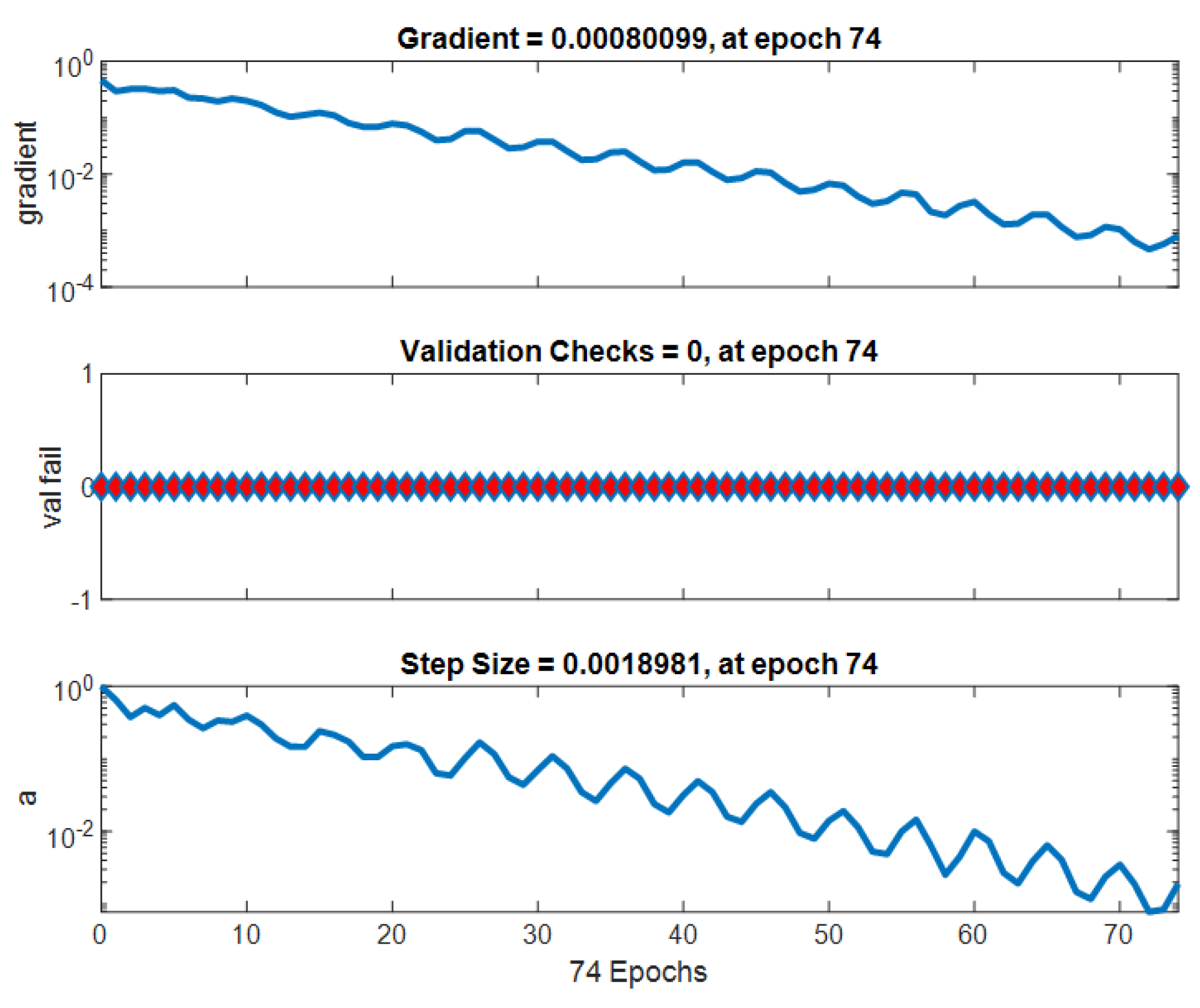
Figure 29 shows the progress of the Taylor neural network training at epoch 74. At this stage, the performance goal has been achieved, meaning the model has converged to an optimal solution according to the specified performance criteria. This suggests that the training process has effectively adjusted the model’s parameters to meet the desired objectives, with a significant reduction in error over the iterations. This figure could also represent the convergence curve, showing the decrease in the cost function or error during the training iterations.

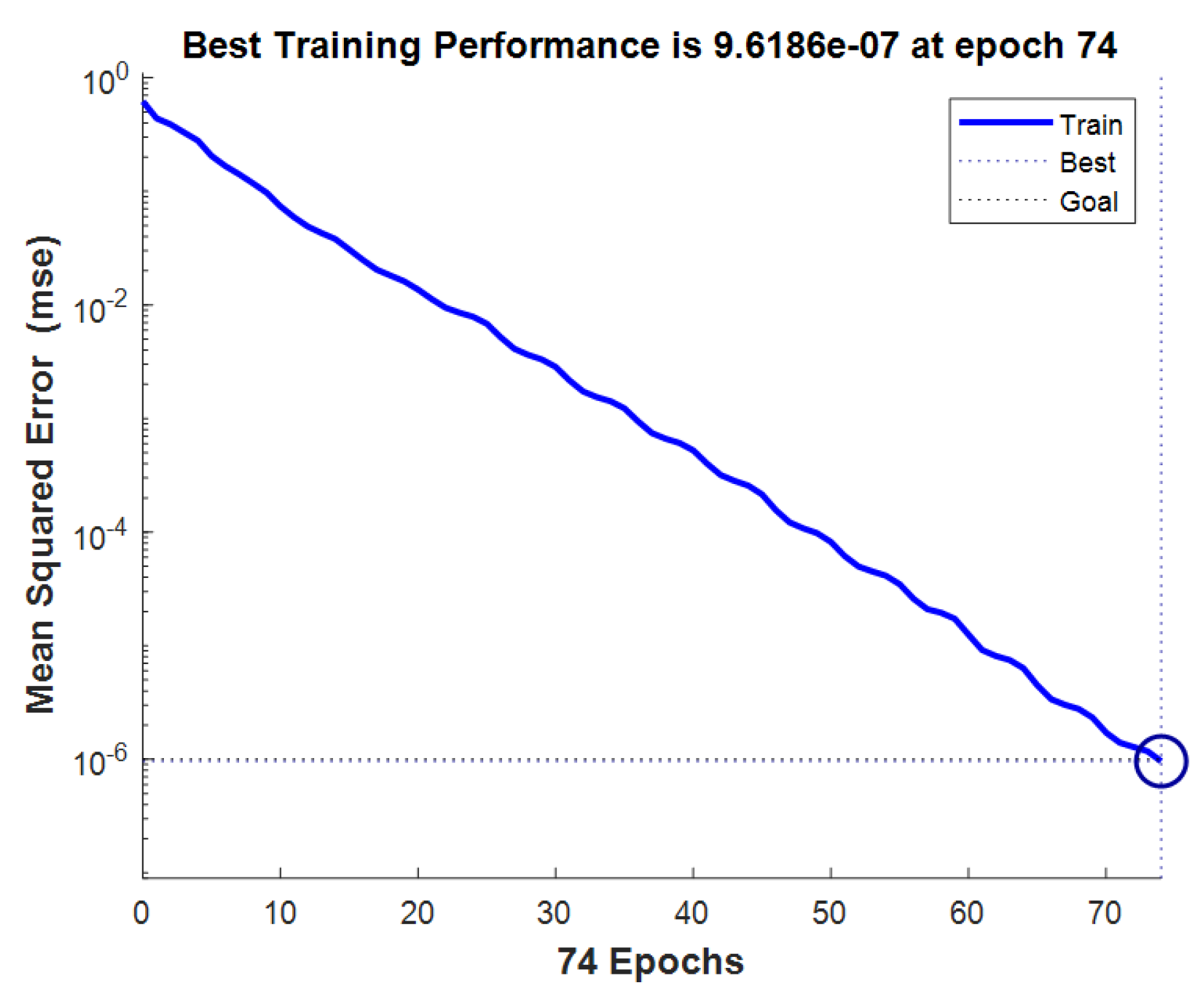
Figure 30 illustrates the evolution of the mean squared error (MSE) for the Taylor neural network. MSE is a key indicator of model quality, measuring the difference between predicted values and actual values. A low MSE indicates good performance, as it shows that the model’s predictions are close to the expected results. This figure likely shows the progressive reduction in the MSE as the neural network learns and adjusts its parameters. A steadily decreasing MSE curve would suggest that the network is effectively converging to a solution with minimal prediction error.

Figure 31 presents the correlation coefficient (R) achieved with the Taylor neural network, which is 0.99999. Such a high correlation coefficient indicates an extremely strong relationship between the predicted values and the actual values. In other words, the model’s predictions are almost identical to the expected results. This level of performance is exceptional and suggests that the model is very well fitted to the training data. A correlation of 0.99999 indicates that the model has learned with great accuracy, which is a strong indicator of the quality of the training and the model’s ability to generalize to new data.

The training process was stopped at epoch 74, where the network reached convergence with minimal loss variation and no further improvement in validation performance, ensuring both efficiency and generalization.

Compared to conventional synthesis approaches, the proposed Taylor–NN method offers a favorable balance between accuracy and computational cost. While methods like PSO and GA require iterative population-based optimization and may take several seconds to converge, the trained neural network provides near-instantaneous inference with high fidelity to the target pattern.

Table 4. Performance comparison of PAA synthesis methods.

Method	Correlation R	SLL (dB)	Computation Time
Chebyshev synthesis	0.96–0.98	−20	∼0.1 s
PSO (heuristic)	0.97–0.99	−23	10–30 s
GA (heuristic)	0.96–0.98	−22	20–60 s
Taylor–NN (ours)	0.99999	−24	<0.1 s (after training)

summarizes these aspects across several popular techniques.

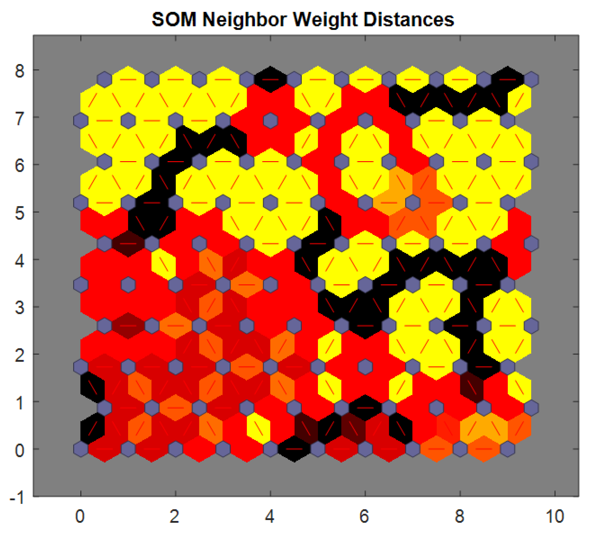
Figure 32 illustrates the SOM (self-organizing map) neighbor weight distances. The SOM is a type of unsupervised neural network used for clustering and dimensionality reduction. In this figure, the distances between the weight vectors of neighboring neurons in the SOM are represented. Each neuron in the SOM has an associated weight vector that represents the characteristics of the data points it maps to. The distances between these weight vectors indicate how similar or different the neurons are in terms of the data they represent. A smaller distance between two neurons suggests that the data points associated with those neurons are similar to each other, while a larger distance indicates greater dissimilarity. This figure likely shows a heatmap or a color-coded representation of the weight distances, where the colors represent the magnitude of the distances. A well-organized SOM would show smaller distances between neurons that are closer to each other on the map, indicating good clustering of similar data points. This figure is crucial for evaluating how the SOM algorithm has grouped the data and how well the structure of the dataset has been captured.

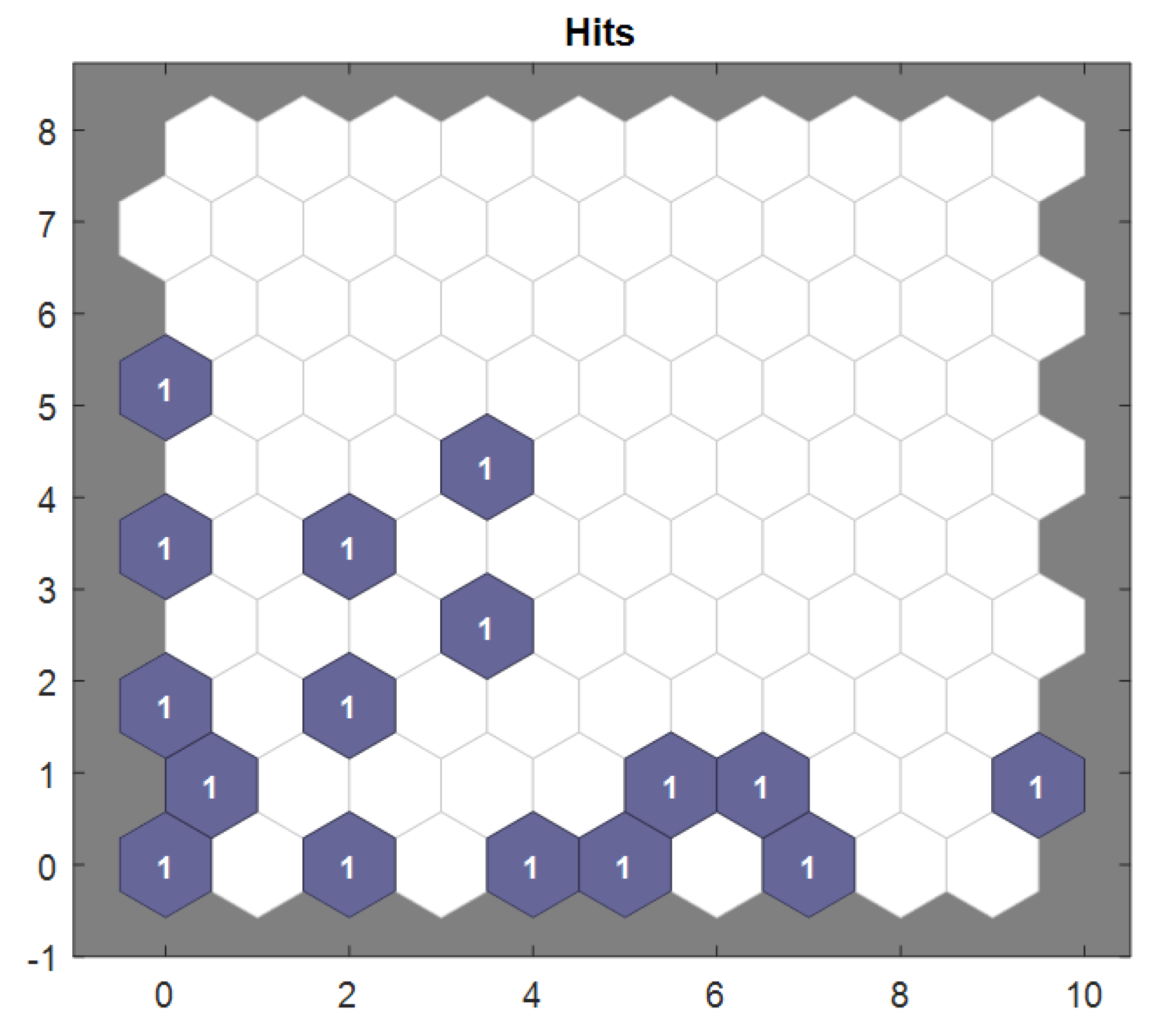
Figure 33 presents the sample hits for the Taylor method dataset. Sample hits refer to the number of data points that have been mapped to each individual neuron in the SOM. In this context, the figure shows a visualization of how frequently each neuron has been activated via the input samples. A high number of hits for a particular neuron indicates that the neuron has been frequently activated via similar data points, suggesting that the neuron represents a dense region or cluster of the dataset. Conversely, a neuron with fewer hits may represent a region in the dataset that is sparsely populated or less representative of the overall data distribution. This figure helps assess the distribution of data across the SOM grid, with areas of the map that have a high number of hits corresponding to well-represented regions of the data. The distribution of hits across the map also reveals how well the SOM has managed to generalize the data into different regions, providing insights into the quality of the clustering. A uniform distribution of hits would indicate a balanced representation of the dataset, whereas a skewed distribution could suggest that some regions of the data are underrepresented or overrepresented in the map. Please refer to the Appendix A for detailed data.

In addition to the benefits discussed above, scalability and future application domains must also be considered. While the current study validates the proposed framework on a 16-element linear array operating at mmWave frequencies (28.14 GHz and 37.88 GHz), the architecture is designed to be scalable and adaptable to more complex configurations, including arrays with 64 elements or more. At such scales, mutual coupling, nonlinear interactions, and hardware-induced uncertainties become more pronounced. These effects can be addressed in future work by incorporating domain-specific mitigation strategies—such as inter-element spacing adjustments, electromagnetic decoupling techniques, or the use of engineered metasurfaces—into the neural network’s training dataset. Furthermore, we aim to extend the applicability of this approach to THz-band antenna arrays, where fabrication tolerances, material dispersion, and surface-wave effects require more intricate modeling. By retraining the network with simulation or measurement-based data that reflect these challenges, the proposed method has the potential to remain robust across a wide range of real-world deployment scenarios.

Beyond scalability, we also recognize that the current focus on uniform linear arrays may limit the generalization of the method to more complex array geometries. Many practical applications involve non-linear configurations, such as conformal, sparse, or irregular arrays—especially in aerospace, vehicular, and satellite systems. While the linear assumption facilitates analytical modeling and initial validation, the proposed Taylor–neural network framework is not intrinsically constrained by geometry. Future developments will extend the approach by incorporating geometric position encodings and training on synthetic datasets representing diverse topologies. These adaptations will enable the model to handle non-uniform or platform-integrated arrays with varying curvature and element spacing. We have explicitly outlined this limitation in the revised manuscript and defined it as a key direction for future research.

6. Conclusions

In conclusion, this paper has presented a novel methodology for the synthesis of phased antenna arrays (PAAs) by combining Taylor-series expansion with neural networks (NNs), achieving notable improvements over traditional techniques. Taylor expansion offers an analytical foundation that simplifies the optimization process by approximating complex radiation behaviors using polynomial expressions. This enables the derivation of more efficient and accurate formulations for beamforming and radiation characteristics. The neural network component complements this by learning the nonlinear relationships between design parameters and target performance metrics, allowing for adaptive tuning and real-time adjustment. The main contributions of this work include the following: (i) the integration of Taylor -series modeling with neural network refinement, (ii) simulation-based validation on a realistic millimeter-wave array, and (iii) performance improvements in sidelobe control and computational efficiency compared to traditional techniques. The proposed method was validated through simulations and an electromagnetic analysis of a 16-element linear array operating at millimeter-wave frequencies (28.14 GHz and 37.88 GHz), ensuring relevance to 5G and 6G use cases. The simulation results demonstrate that the hybrid Taylor–NN framework reduces computational complexity, enhances adaptability, and enables broader design-space exploration. The validation confirms the method’s practical potential for the design of efficient antenna arrays in advanced communication and radar systems. It is worth noting that, although experimental measurements were not included in the current study, the simulation framework was built upon detailed electromagnetic modeling using realistic substrate and layout parameters. Future investigations may involve hardware prototyping and empirical validation as part of an extended deployment-oriented study.

While the current work focused on uniform linear arrays, we acknowledge its present limitations in addressing more complex configurations such as conformal or sparse geometries, which are prevalent in aerospace and vehicular applications. Future extensions will target these scenarios by incorporating non-linear geometries, generalized position encoding, and data-driven training strategies. This work marks a significant advancement in phased antenna array synthesis, highlighting the benefits of integrating analytical modeling with artificial intelligence to enable robust and flexible antenna design. By integrating scalability, adaptability, and extensibility into the design pipeline, the proposed approach provides a promising solution to modern challenges in wireless communication and radar engineering. Although experimental measurements are not included in the current study, the simulation framework is built upon detailed electromagnetic modeling using realistic substrate and layout parameters. Future investigations may involve hardware prototyping and empirical validation as part of an extended deployment-oriented study.