Article

Experimental Model Development for the Attenuation Coefficient Estimation of Terrestrial Optical Wireless Links over the Sea

by
Argyris N. Stassinakis
1,
George A. Papavgeris
1,
Hector E. Nistazakis
1,*,
Andreas D. Tsigopoulos
2,
Nikolaos A. Androutsos
1 and
George S. Tombras
1
1
Section of Electronic Physics and Systems, Department of Physics, National and Kapodistrian University of Athens, 15784 Athens, Greece
2
Department of Battle Systems, Naval Operations, Sea Studies, Navigation, Electronics and Telecommunications, Hellenic Naval Academy, Hadjikyriakouave, 18539 Piraeus, Greece
*
Author to whom correspondence should be addressed.
Telecom 2021, 2(1), 93-107; https://doi.org/10.3390/telecom2010007
Submission received: 31 December 2020 / Revised: 11 February 2021 / Accepted: 18 February 2021 / Published: 1 March 2021
(This article belongs to the Special Issue Modern Circuits and Systems Technologies on Communications 2020)

Abstract

:
Free space optical (FSO) systems have become a reliable solution for modern communications networks, due to the high performance, availability, reliability and security they can provide. However, their characteristics depend strongly on the conditions of the atmosphere, which is the propagation path of the optical beam. In this work, this dependence is experimentally investigated through a terrestrial horizontal FSO link, which was installed a few meters above the sea. Thus, the procedure presented hereis an accurate empirical model for the estimation of the attenuation coefficient for an optical wireless link, as a function of the atmospheric temperature, the relative humidity, and the wind speed. Its accuracy is verified by comparing the estimated outcomes—obtained from the empirical model—versus the measured—experimental—ones. Such accurate empirical models can be used for designing high performance and reliability FSO links, as parts of the upcoming 5G/5G+ networks, for areas where the behavior of the atmospheric conditions and parameters are known.

1. Introduction

During the last few decades, free space optical (FSO) systems attracted very significant research and commercial interest, due to the plenty of advantages they can offer and the development margins they show. The high data rate transmission and security level they offer, along with the relatively low operational cost and the license free installation, are some reasons why the FSO links are part of the modern communication networks, i.e., 5G/5G+ [1,2].
On the other hand, the performance, the reliability, and the availability of the FSO systems, strongly depend on the atmospheric and weather conditions as the laser beam propagates through the atmosphere. An important factor that affects the performance of FSO links is attenuation due to absorption and scattering, which might cause serious performance degradation or even outages, in cases of dense fog or rain [3,4,5,6]. Furthermore, another factor that deteriorates the performance of the FSO links is the atmospheric turbulence that causes the scintillation effect [7,8,9,10,11,12]. All these factors were extensively studied in a theoretical way and various channel models were extracted in order to estimate the main metrics of a communication system, such as the outage probability, the bit error rate, etc. [13,14,15,16,17].
During the last years, various experimental FSO links were deployed in order to validate the accuracy of many theoretical models, and at the same time, extract empirical models for the attenuation estimation of optical power, in specific cases [18,19,20,21,22,23,24,25,26,27,28,29,30,31]. In this work, a novel empirical experimental model for the attenuation coefficient was extracted using a multiple linear regression method for the maritime environment during night-time, as a function of the atmospheric temperature, the relative humidity, and the wind speed. Various regression techniques are already used in order to extract empirical models in FSO communications [29,30,31]. The presence of sea water below the FSO link creates weak to strong turbulence conditions, due to water vaporization and high attenuation due to high levels of humidity. Therefore, it is important to extract a model that predicts the communications’ quality of an FSO system, in an environment with such a great impact on its performance. Its accuracy was validated by comparing the estimated attenuation coefficient results versus the real ones, which were obtained from measurements.
The remainder of this work is organized as follows. In Section 2, the theoretical background is mentioned, while in Section 3, the experimental setup is presented. Next, in Section 4, the experimental model is derived and its results are presented. Finally, the conclusions of this work are presented in Section 5.

2. Theoretical Analysis of the Model

As the optical beam propagates through the atmospheric channel, the geometrical losses, the scattering, the absorption, and the turbulence are the most significant attenuation parameters.

2.1. Geometrical Losses Attenuation

An important factor that reduces the useful optical power that arrives at the receiver is the attenuation due to geometrical losses, and depends on the technical parameter values of the transceivers and the link’s length. Specifically, the geometrical loss factor, aGL, could be estimated as [4,24]:
a G L = ( D r D r + θ l ) 2
where Dr and Dt represent the aperture diameter of the receiver and transmitter, respectively, θ is the divergence angle and l stands for the link’s length. Thus, using Equation (1), the received optical power is estimated as [4,24]:
P r G L = a G L P t
with PrGL and Pt being the optical power at the receiver,due to geometrical losses and the transmitter, respectively. For terrestrial ground-to-ground FSO links where their length remains invariable, the geometrical loss factor is constant.

2.2. Atmospheric Attenuation

The laser beam propagation through the atmosphere causes attenuation of the optical power due to scattering, absorption, and turbulence. Thus, many accurate theoretical and empirical models for the estimation of the corresponding coefficients, i.e., asc, aab, atur, were proposed and verified [18,32]. Furthermore, in order to estimate thetotal received optical power, Pr, due to the total atmospheric attenuation, atot, the Beer-Lambert’s law equation was used [3,4,24,32]:
P r = P r G L exp ( a t o t l )
where atot = asc + aab + atur. Then, using Equations (2) and (3), the total attenuation factor, atot, could be estimated through the link’s parameters and characteristics, as:
a t o t = 1 l l n ( P r a G L P t )

3. Experimental Setup

The experimental setup thatwas used here is a terrestrial horizontal FSO link that was installed in the Piraeus port in Greece, connecting a building of the Hellenic Naval Academy and the lighthouse of the island of Psyttaleia. The link appears in Figure 1, while the corresponding technical characteristics were adjusted to take on the values presented in Table 1.
In order to achieve precise alignment between the FSO transceivers during the installation, the scopes of the devices were used in order to receive the maximum power at each side. The received optical signal was transformed into voltage signal that was proportional to the square root of the optical power, see Appendix A. This voltage represented the received signal strength indicator (RSSI) and it could be monitored through the software of the FSO device. The values of RSSI and the time were recorded and saved in the internal storage of the FSO head, every thirty seconds. Following the procedure that appeared in Appendix A, the RSSI values could be transformed into optical power measurements. This accurate transformation is necessary as the transmitted power cannot easily transform to the RSSI units. Taking into account the transmitted and the received optical power, the attenuation factor could be evaluated from Equation (4).
The RSSI values strongly depend on weather and atmospheric conditions. Therefore, by installing a precise meteorological station close to the FSO transceivers, various meteorological parameters were measured, with temperature, relative humidity, and wind speed being the ones that most affect the laser beam propagation [4,13,14,18,19]. Another factor that affects the attenuation is the link’s operational wavelength which was invariable in the experimentsin this work.
The experimental measurements were collected continuously for more than a six-months time-period. However, in order to decrease the degrees of freedom of the specific problem that we studied and to obtain accurate results, we tried to examine cases where the influence of the sunlight radiation could be assumed to be negligible. Thus, in this work, we used the data that corresponded to time-periods between 8:00 p.m. to 5:00 a.m. For the same reason, measurements with nonzero precipitations were also excluded. Specifically, the experimental data that were used in this work are the ones that met the criteria that appeared in Table 2.

4. Model Analysis and Results

By substituting the experimental values of transmitted and received optical powerin Equation (4), the experimental attenuation coefficient was evaluated. According to existing models for turbulence and attenuation in FSO systems, the main meteorological factors that affect the propagation of the laser beam were the relative humidity, temperature, and wind speed [4,13,14,18,19]. Thus, the experimental model for the estimation of the attenuation factor would depend on these three parameters and was extracted using multiple linear regression method with the attenuation coefficient being the dependent variable and combinations of up to 3rd order values of temperature, wind speed, and relative humidity being the explanatory variables xi [33]:
a t o t = b 0 + i = 1 N b i x i
Data collected in the first three months of the year 2020 were used for the regression process for time-periods that fulfilled the requirements of Table 2.
In order to simplify the regression model, factors with a negligible contribution were eliminated. Thus, the estimation model for the attenuation coefficient as a function of atmospheric temperature, relative humidity, and wind speed is given through the following mathematical expression:
a t o t = b 0 + b 1 R H 4 + b 2 R H 4 T 3 + b 3 T 4 + b 4 R H 2 T W S + b 5 R H 2 + b 6 W S 2 + b 7 T 2 + b 8 R H 3 + b 9 T 3 + b 10 R H × T 2 W S + b 11 R H 2 T + b 12 R H 2 T 2 + b 13 R H 3 T 2
where T stands for the temperature in Celsius degrees, RH corresponds to the relative humidity, and WS represents the wind speed in m/s. The values of the coefficients of Equation (6) are presented in Table 3.
Taking into account the parameter values of Table 3, the validity and the error parameters of the experimental model are presented in Table 4.
From Table 4, it can be seen that the coefficient of multiple correlation that is the most important parameter for the fitting accuracy of the model is close enough to one, so the accuracy of the model is high enough. Furthermore, the residual mean variance is very low, three orders of magnitude lower that the experimental measurements, a sign of high precision model.
Next, the outcomes for the attenuation factor obtained from the experiment and those that were obtained from the empirical model of Equation (6), were compared.
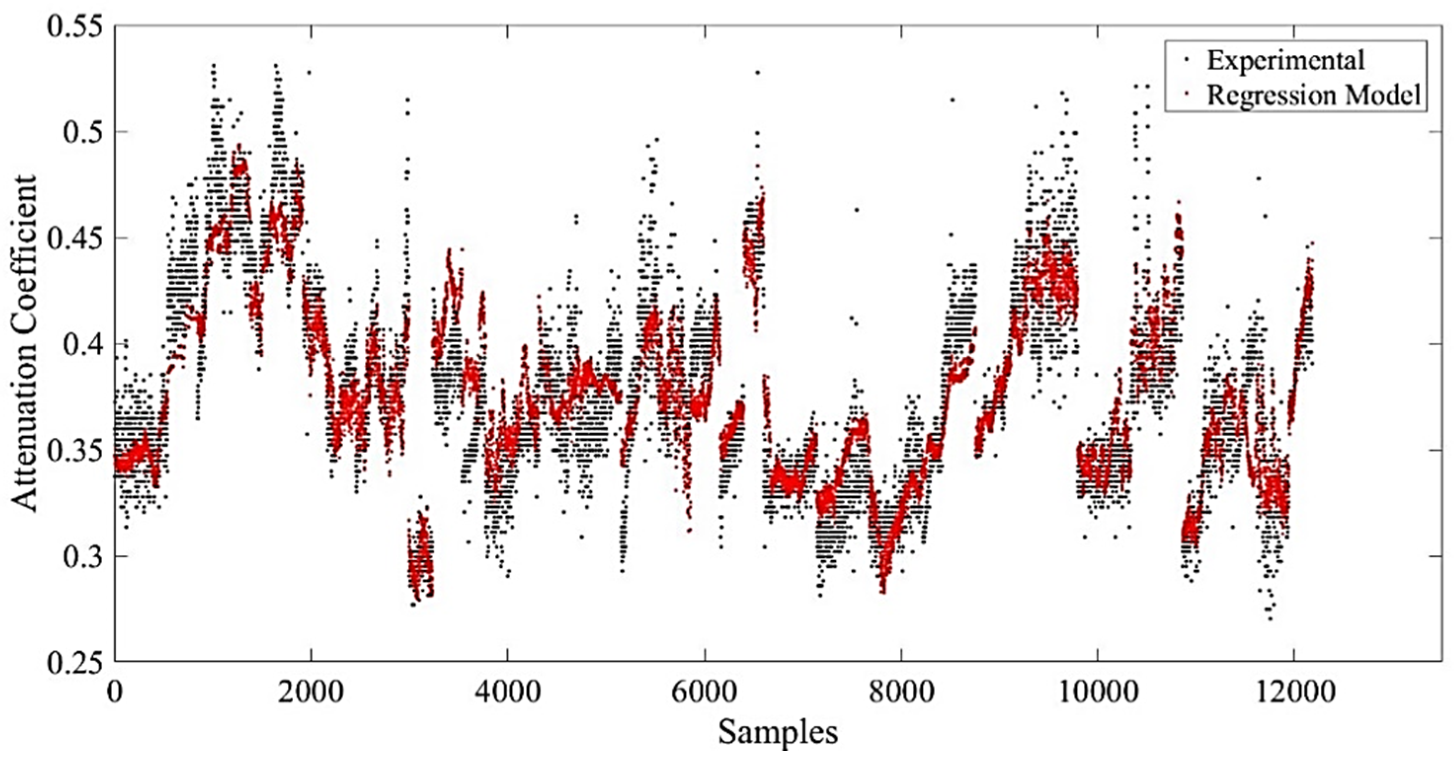
In Figure 2, the experimental measurements of the attenuation coefficient according to Εquation (4) and the predicted values of the regression model of Εquation (6) were presented for 12,300 samples. It could be observed that the model that was extracted had a precise fit to the behavior of the experimental results and could predict the attenuation coefficient according to weather and atmospheric data. In 
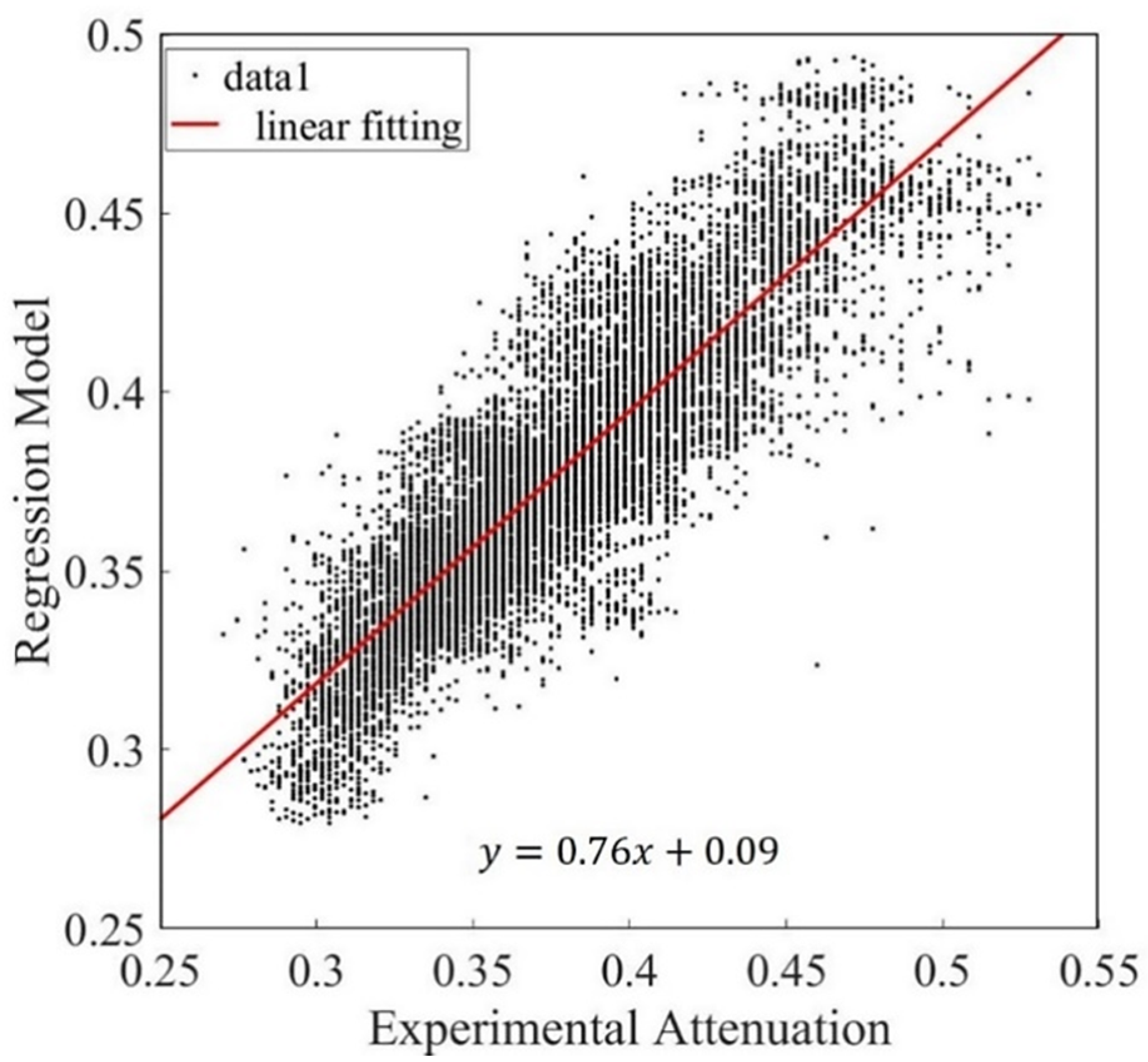
Figure 3, the experimental versus the corresponding regression model results are presented. According to the linear fitting, the slope of the curve was 0.7612 and was near to 1, as it should theoretically be, while the constant term was very low, i.e., 0.09. It could also be seen, that as the attenuation coefficient increased, the accuracy of the model decreased. This was expected because an increment of attenuation coefficient meant worse weather conditions that could not be easily modelled.
In 
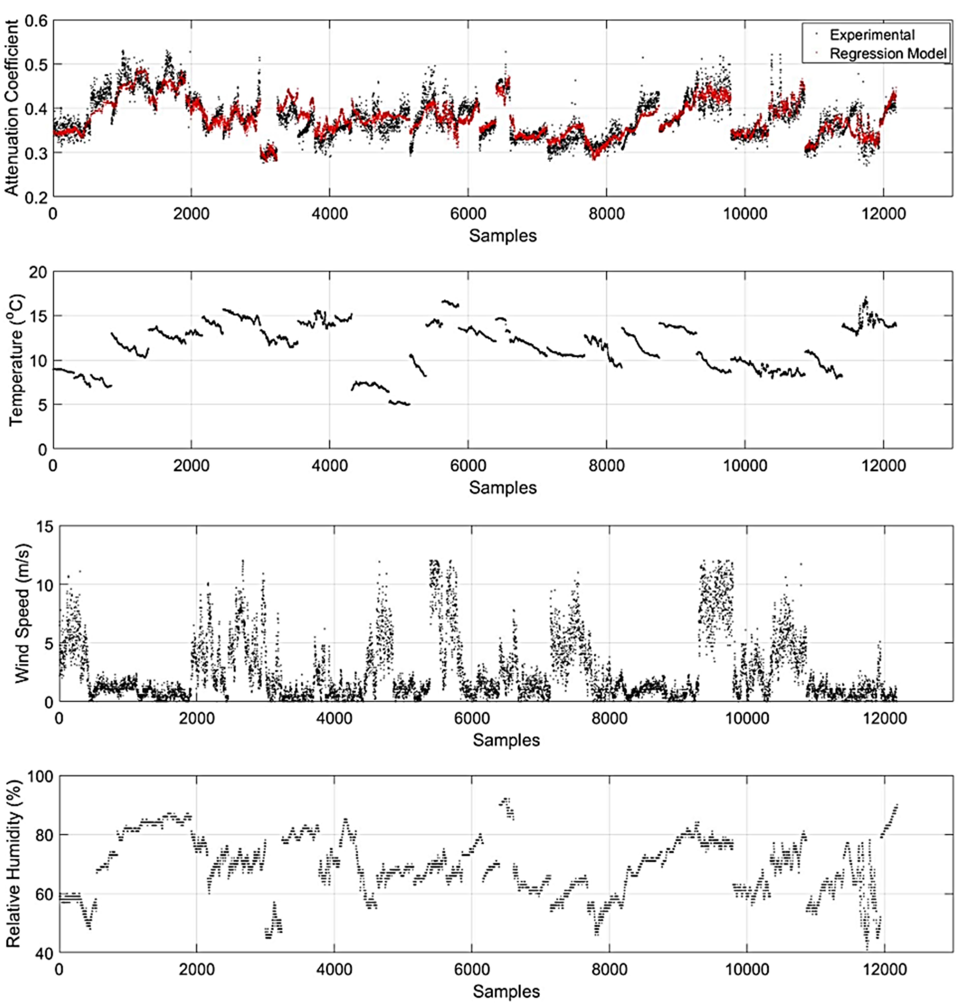
Figure 4, the measurements of temperature, wind speed, and relative humidity are presented for every sample that was used for the extraction of the model. It could be observed that the model has a high accuracy in case of low wind speed and relative humidity. In contrary, high values of such parameters that are responsible for very high attenuation and create fast changes in the consistency of the atmosphere, decrease the accuracy of the model. Furthermore, temperature affects the accuracy of the model in cases of very low values.
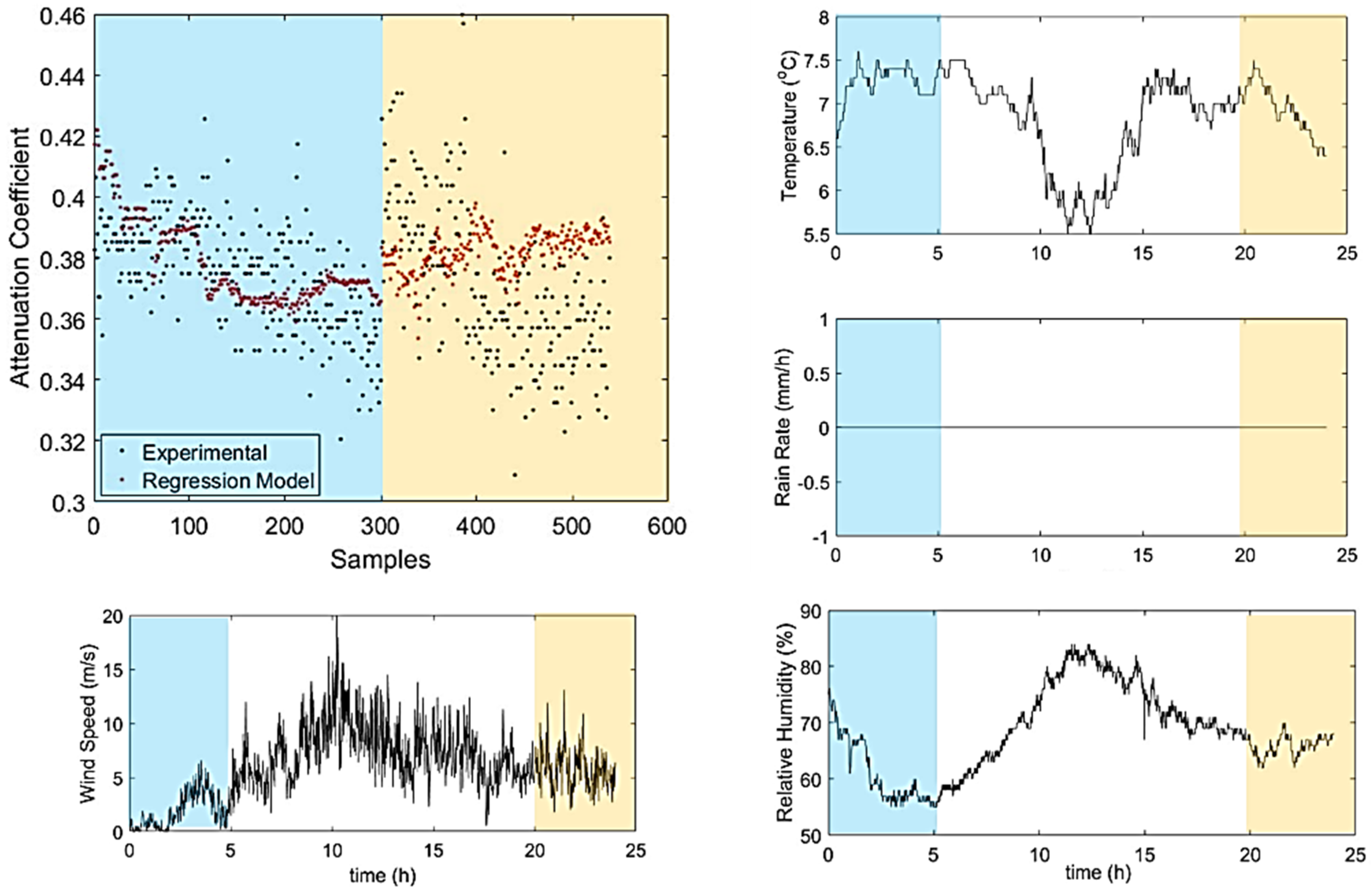
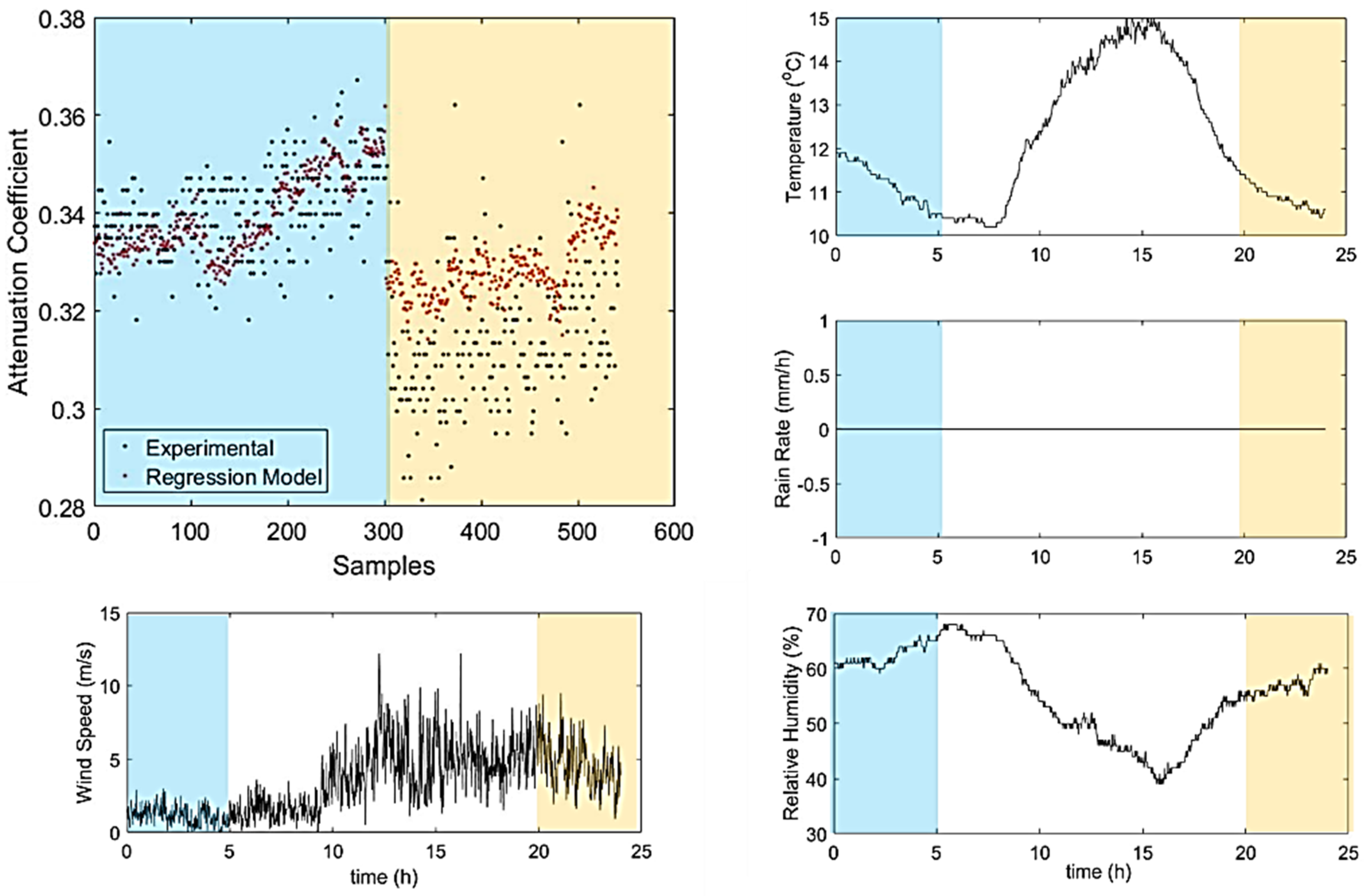
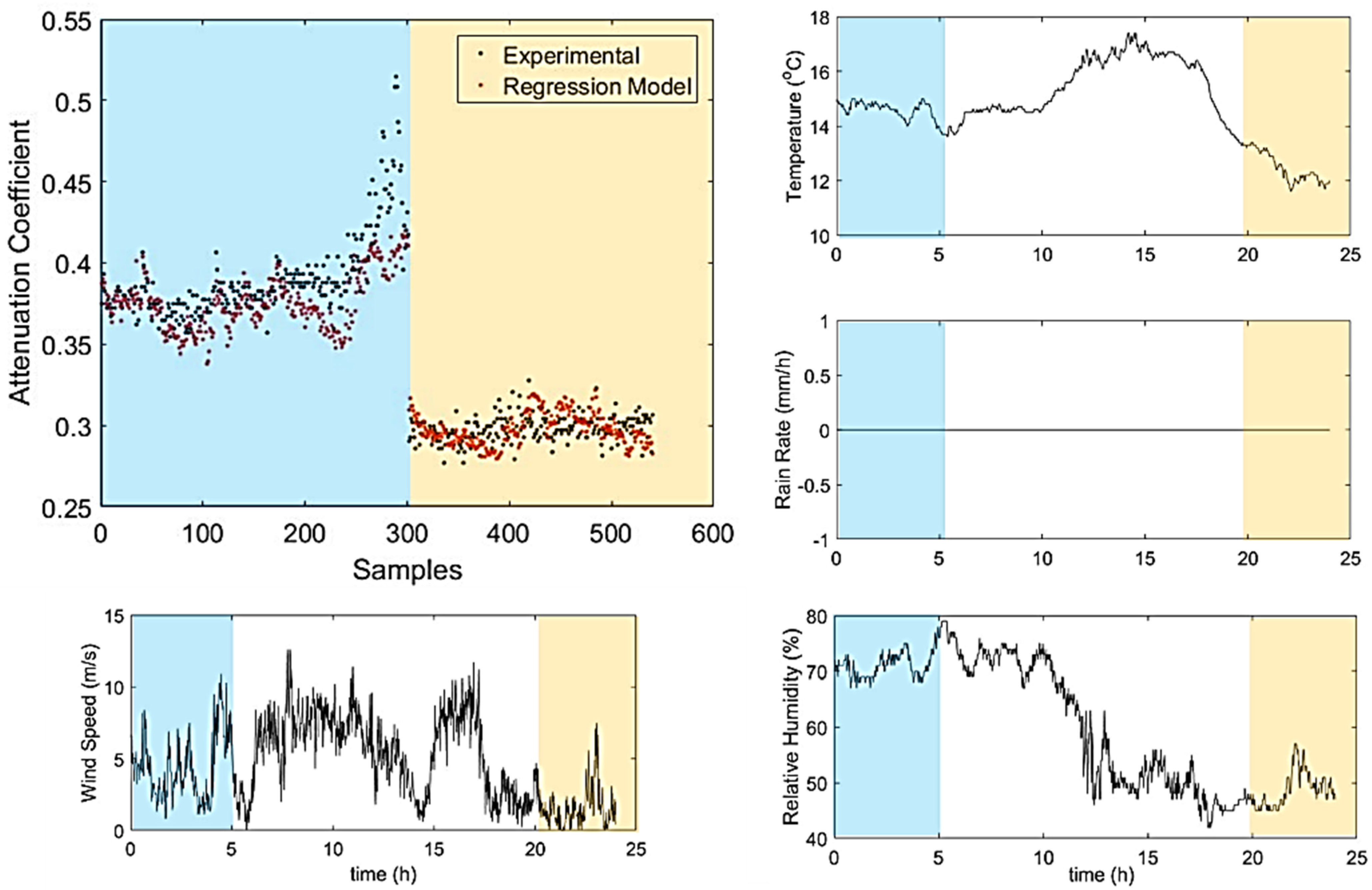
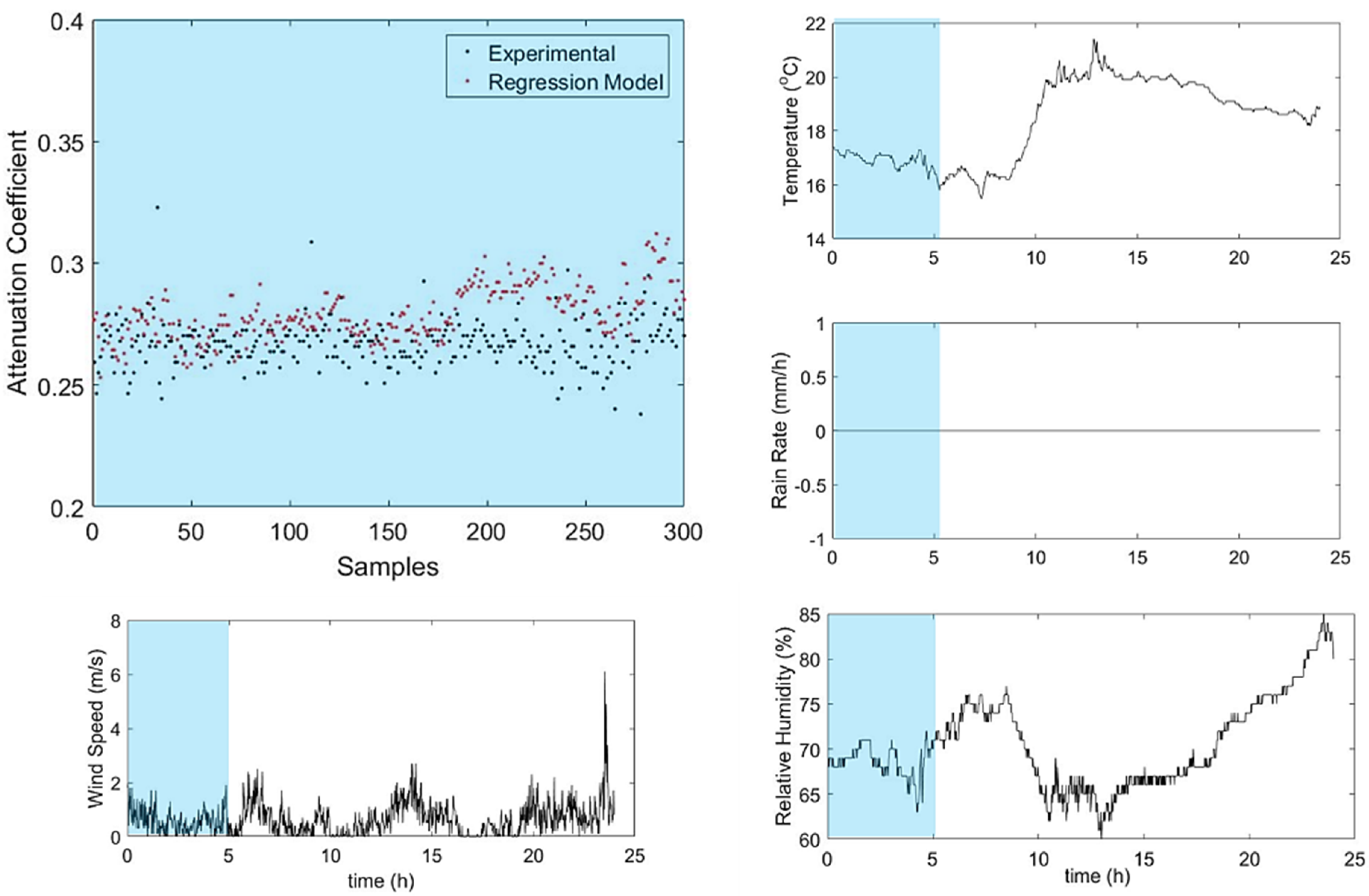
In order to more precisely investigate the behavior of the model in various weather conditions, the results of empirical model and experimental measurements are presented for specific days. In the blue box are the measurements between 00:00 a.m. to 05:00 a.m., while in the orange one are the measurements between 8:00 pm to 11:59 p.m. At the right side of the Figure 5, Figure 6, Figure 7, Figure 8, Figure 9, Figure 10 and Figure 11, the wind speed and the rain rate are presented for the whole day.
In Figure 5 and Figure 6, the results of windy nights are presented. It could be observed that between 00:00 and 05:00 the wind was lower than 5 m/s, the model had a good fitting, while between 20:00 and 23:59, the wind was over 5 m/s with severe gusts, where the model diverged more, but was still close to the experimental measurements.
In Figure 7, it can be observed that a lack of accuracy before precipitation took place due to unstable and fast changes in weather conditions. It was clear that the very high value of the relative humidity decreased the accuracy of the model, as the attenuation coefficient was very high. On the other hand, between 21:00 and 23:59, a few hours after precipitation and with very low wind speed where the weather conditions were mild and stable, the model presented a very high accuracy.
In Figure 8, the results of the model are presented in cases of sudden and severe wind gusts and changes. Between 00:00 and 05:00, this phenomenon was more severe and at the same time, the relative humidity increased and the model lacked accuracy in some cases. However, as shown in Figure 6, between 20:00 and 23:59, the model showed very high accuracy in predicting the attenuation coefficient due to mild conditions.
The partial coefficient of multiple correlation, R2, is presented in the following Table 5, for the days presented in Figure 5, Figure 6, Figure 7 and Figure 8.
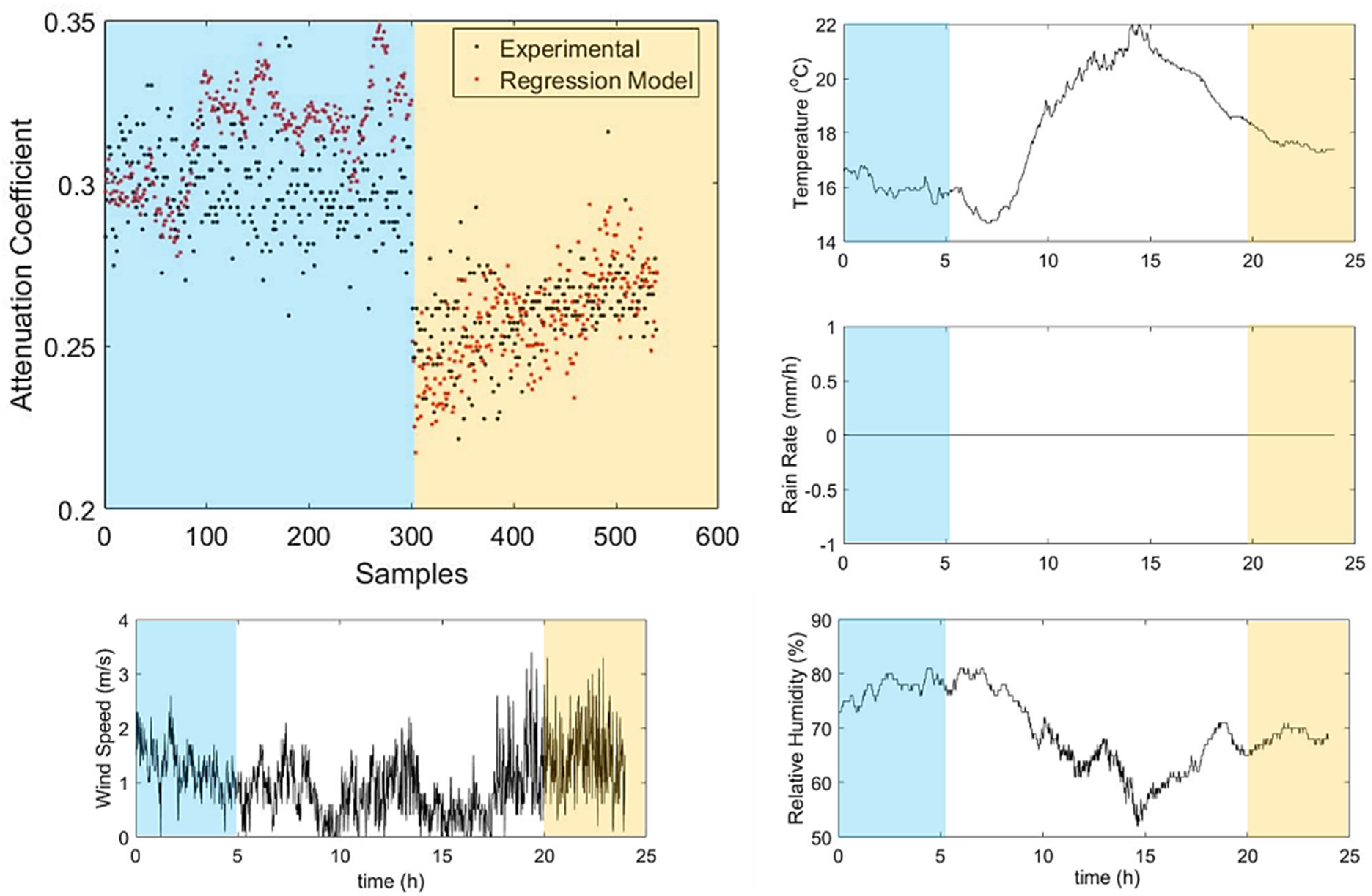
In order to further validate the accuracy of the model, we applied it in days that were not included in the data of the regression process. We chose days with a wide variety of weather conditions, in order to observe the models behavior, and the results are presented in Figure 9, Figure 10 and Figure 11.
From the experimental measurements and the predictions of the empirical model of Equation (6), of Figure 9, Figure 10 and Figure 11, it can be seen that they follow the same behavior as those of Figure 5, Figure 6, Figure 7 and Figure 8. Specifically, the model is very accurate in cases of both low wind speedand relative humidity, without precipitations and diverges in more severe weather changes. The values of R2 for the days that were not used in the regression method for the extraction of the model are presented in Table 6, as follows:
In Figure 11, the FSO link was switched off for safety reasons at night, due to a ship that was expected to pass through the propagation path of the LASER beam, so only measurements between 00:00 and 05:00 were collected. Thus, the model proved to be accurate enough under specific constraints, and it could be used in order to predict the performance of FSO links, in real maritime environment, during night.
Finally, we examined the mean value and the standard deviation of the experimental attenuation coefficient for almost the same values of temperature, wind speed, and relative humidity, respectively; the results are presented in the following Table 7.
According to Table 7, it is clear that the attenuation coefficient mostly depended on temperature, wind speed, and relative humidity, as the standard deviation in cases of almost same values of these parameters was very low. On the other hand, the model might become more accurate if more atmospheric and weather parameters, i.e., atmospheric pressure, are investigated.

5. Conclusions

In this work, an empirical experimental model for the attenuation coefficient estimation of an FSO system, which operates in low height over the sea, during night-time, was presented as a function of the atmospheric temperature, the wind speed, and the relative humidity. According to the obtained results that were presented, the model achieved very high accuracy in cases with low wind speed, low relative humidity, high temperature, and without precipitations where the attenuation coefficient was relatively low. Such an empirical model is a very useful tool in order to predict the performance and reliability of an FSO link, in a specific environment with known characteristics and has a great impact in the designing of high demanding modern communication networks.

Author Contributions

Conceptualization, A.N.S., G.A.P., H.E.N., A.D.T. and N.A.A.; methodology, A.N.S., G.A.P. and H.E.N.; software, A.N.S. and G.A.P.; validation, A.N.S., G.A.P., H.E.N., A.D.T., N.A.A. and G.S.T.; formal analysis, A.N.S. and G.A.P.; investigation, A.N.S., G.A.P. and N.A.A.; resources, A.N.S., G.A.P., H.E.N., A.D.T., N.A.A. and G.S.T.; writing—original draft preparation, A.N.S. and G.A.P.; writing—review and editing, A.N.S., G.A.P., H.E.N., A.D.T., N.A.A. and G.S.T.; visualization, A.N.S. and G.A.P.; supervision, A.N.S., H.E.N., A.D.T. and G.S.T.; project administration, A.N.S., H.E.N., A.D.T. and G.S.T.; funding acquisition, H.E.N., G.S.T. and N.A.A. All authors have read and agreed to the published version of the manuscript.

Funding

H.E.N. and G.S.T. acknowledge that this work received funding from the European Union’s Horizon 2020 research and innovation program, under grant agreement No: 871900. N.A.A. acknowledges that this research was co-financed by Greece and the European Union (European Social Fund- ESF) through the Operational Program “Human Resources Development, Education and Lifelong Learning”, in the context of the project “Strengthening Human Resources Research Potential via Doctorate Research” (MIS-5000432), implemented by the State Scholarships Foundation (ΙΚΥ).

Data Availability Statement

Data available on request due to restrictions eg privacy or ethical. The data presented in this study are available on request from the corresponding author. The data are not publicly available as the experiment was held in a military base.

Conflicts of Interest

The authors declare no conflict of interest.

Appendix A

According to the official manual of the FSO device, the connection between the RSSI values and the link length, i.e., distance, appears in Figure 11.
Figure A1. RSSI as a function of distance.
Telecom 02 00007 g0a1
The attenuation of this diagram was estimated according to the geometrical losses of the link using Equation (1).
According to Reference [34], the voltage at the output of an electronic circuit was proportional to the square root of the optical power received. Therefore, the RSSI as a function of the received optical power is given in Figure A1.
Figure A2. RSSI and Optical power linear fitting.
Telecom 02 00007 g0a2
Using the linear fitting technique the optical power received could be estimated as:
P r = ( 0.023078 R S S I 0.0036 ) 2

References

  1. Pham, A.T.; Trinh, P.V.; Mai, V.V.; Dang, N.T.; Truong, C.-T. Hybrid free-space optics/millimeter-wave architecture for 5G cellular backhaul networks. In Proceedings of the 2015 Opto-Electronics and Communications Conference (OECC), Shanghai, China, 28 June–2 July 2015; pp. 1–3. [Google Scholar] [CrossRef]
  2. Malik, S.; Sahu, P.K. Free space optics/millimeter-wave based vertical and horizontal terrestrial backhaul network for 5G. Opt. Commun. 2020, 459, 0030–4018. [Google Scholar] [CrossRef]
  3. Gebhart, M.; Leitgeb, E.; Sheikh Muhammad, S.; Flecker, B.; Chlestil, C.; Al Naboulsi, M.; de Fornel, F.; Sizun, H. Measurement of light attenuation in dense fog conditions for FSO applications. In Proceedings of the SPIE 5891, Atmospheric Optical Modeling, Measurement, and Simulation, 58910K, San Diego, CA, USA,, 18 August 2005. [Google Scholar] [CrossRef]
  4. Ghoname, S.; Fayed, H.A.; El Aziz, A.A.; Aly, M.H. Performance analysis of FSO communication system: Effects of fog, rain and humidity. In Proceedings of the 2016 Sixth International Conference on Digital Information Processing and Communications (ICDIPC), Beirut, Lebanon, 21–23 April 2016; pp. 151–155. [Google Scholar] [CrossRef]
  5. Nadeem, F.; Flecker, B.; Leitgeb, E.; Khan, M.S.; Awan, M.S.; Javornik, T. Comparing the fog effects on hybrid network using optical wireless and GHz links. In Proceedings of the 2008 6th International Symposium on Communication Systems, Networks and Digital Signal Processing, Graz, Austria, 25 July 2008; pp. 278–282. [Google Scholar] [CrossRef]
  6. Leitgeb, E.; Gebhart, M.; Fasser, P.; Bregenzer, J.; Tanczos, J. Impact of atmospheric effects in Free Space Optics Transmission systems. In Proceedings of the High-Power Lasers and Applications, San Jose, CA, USA, 25–31 January 2003; Volume 4976-28. [Google Scholar]
  7. Nistazakis, H.E.; Tsiftsis, T.A.; Tombras, G.S. Performance analysis of free-space optical communication systems over atmospheric turbulence channels. IET Commun. 2009, 3, 1402. [Google Scholar] [CrossRef]
  8. Peppas, K.P. A Simple, Accurate Approximation to the Sum of Gamma–Gamma Variates and Applications in MIMO Free-Space Optical Systems. IEEE Photon.-Technol. Lett. 2011, 23, 839–841. [Google Scholar] [CrossRef]
  9. Datsikas, C.K.; Peppas, K.P.; Sagias, N.C.; Tombras, G.S. Serial Free-Space Optical Relaying Communications Over Gamma-Gamma Atmospheric Turbulence Channels. J. Opt. Commun. Netw. 2010, 2, 576–586. [Google Scholar] [CrossRef]
  10. Stassinakis, A.; Nistazakis, H.; Peppas, K.; Tombras, G. Improving the availability of terrestrial FSO links over log normal atmospheric turbulence channels using dispersive chirped Gaussian pulses. Opt. Laser Technol. 2013, 54, 329–334. [Google Scholar] [CrossRef]
  11. Ninos, M.; Nistazakis, H.; Tombras, G. On the BER performance of FSO links with multiple receivers and spatial jitter over gamma-gamma or exponential turbulence channels. Optik 2017, 138, 269–279. [Google Scholar] [CrossRef]
  12. Varotsos, G.K.; Nistazakis, H.E.; Gappmair, W.; Sandalidis, H.G.; Tombras, G.S. DF relayed subcarrier FSO links over Malaga turbulence channels with phase noise and non-zero boresight pointing errors. Appl. Sci. 2018, 8, 664. [Google Scholar] [CrossRef] [Green Version]
  13. Bang, C.-H.; Lee, J.; Hong, S.-Y. Predictability Experiments of Fog and Visibility in Local Airports over Korea using the WRF Model. J. Korean Soc. Atmos. Environ. 2008, 24, 92–101. [Google Scholar]
  14. Al-Gailani, S.A.; Mohammad, A.B.; Islam, M.S.; Sheikh, U.U.; Shaddad, R.Q. Tropical temperature and humidity modeling for free space optical link. J. Opt. 2015, 45, 87–91. [Google Scholar] [CrossRef]
  15. Ijaz, M.; Ghassemlooy, Z.; Pesek, J.; Fiser, O.; Le Minh, H.; Bentley, E. Modeling of Fog and Smoke Attenuation in Free Space Optical Communications Link Under Controlled Laboratory Conditions. J. Light. Technol. 2013, 31, 1720–1726. [Google Scholar] [CrossRef]
  16. Ghassemlooy, Z.; Popoola, W.O.; Leitgeb, E. Free-Space Optical Communication Using Subcarrier Modulation in Gamma-Gamma Atmospheric Turbulence. In Proceedings of the 2007 9th International Conference on Transparent Optical Networks, Rome, Italy, 1–5 July 2007; pp. 156–160. [Google Scholar] [CrossRef]
  17. Stassinakis, A.N.; Nistazakis, H.E.; Tombras, G.S. Comparative performance study of one or multiple receivers schemes for FSO links over gamma–gamma turbulence channels. J. Mod. Opt. 2012, 59, 1023–1031. [Google Scholar] [CrossRef]
  18. Raj, A.A.B.; Selvi, J.A.V.; Durairaj, S. Comparison of different models for ground-level atmospheric turbulence strength (Cn2) prediction with a new model according to local weather data for FSO applications. Appl. Opt. 2015, 54, 802–815. [Google Scholar]
  19. Deng, H.; Tan, H.; Li, F.; Cai, M.; Chan, P.; Xu, H.; Huang, X.; Wu, D. Impact of relative humidity on visibility degradation during a haze event: A case study. Sci. Total Environ. 2016, 569–570, 1149–1158. [Google Scholar] [CrossRef] [PubMed]
  20. Kruse, P.W. Elements of Infrared Technology: Generation, Transmission and Detection; Wiley and Sons: New York, NY, USA, 1962. [Google Scholar]
  21. Kim, I.I.; McArthur, B.; Korevaar, E.J. Comparison of laser beam propagation at 785 nm and 1550 nm in fog and haze for optical wireless communications. In Proceedings of the SPIE 4214, Optical Wireless Communications III, Boston, MA, USA, 6 February 2001. [Google Scholar] [CrossRef]
  22. Latal, J.; Hajek, L.; Vanderka, A.; Vitasek, J. Regresion models utilization for RSSI prediction of professional FSO link with regards to atmosphere phenomena. In Proceedings of the 2016 International Conference on Broadband Communications for Next Generation Networks and Multimedia Applications (CoBCom), Graz, Austria, 14–16 September 2016; pp. 1–6. [Google Scholar] [CrossRef]
  23. Grabner, M.; Kvicera, V. The wavelength dependent model of extinction in fog and haze for free space optical communication. Opt. Express 2011, 19, 3379–3386. [Google Scholar] [CrossRef]
  24. Alheadary, W.G.; Park, K.-H.; Alfaraj, N.; Guo, Y.; Stegenburgs, E.; Ng, T.K.; Ooi, B.S.; Alouini, M.-S. Free-space optical channel characterization and experimental validation in a coastal environment. Opt. Express 2018, 26, 6614–6628. [Google Scholar] [CrossRef] [Green Version]
  25. Lionis, A.; Peppas, K.; Nistazakis, H.E.; Tsigopoulos, A.D.; Cohn, K. Experimental Performance Analysis of an Optical Communication Channel over Maritime Environment. Electronics 2020, 9, 1109. [Google Scholar] [CrossRef]
  26. Moore, C.I.; Burris, H.R.; Stell, M.F.; Wasiczko, L.; Suite, M.R.; Mahon, R.; Rabinovich, W.S.; Gilbreath, G.C.; Scharpf, W.J. Atmospheric turbulence studies of a 16-km maritime path. In Proceedings of the SPIE 5793, Atmospheric Propagation II, Orlando, FL, USA, 25 May 2005. [Google Scholar]
  27. Grant, K.J.; Mudge, K.A.; Clare, B.A.; Perejma, A.S.; Martinsen, W.M. Maritime Laser Communications Trial 98152-19703. In Command, Control, Communications and Intelligence Division; DSTO: Edinburgh, Australia, 2012. [Google Scholar]
  28. Latal, J.; Hajek, L.; Vanderka, A.; Vitasek, J.; Koudelka, P.; Hejduk, S. Real Measurements and Evaluation of the Influence of Atmospheric Phenomena on FSO Combined with Modulation Formats. Electron. ETF 2017, 20, 62–68. [Google Scholar] [CrossRef] [Green Version]
  29. Esmail, M.A.; Fathallah, H.; Alouini, M.-S. An Experimental Study of FSO Link Performance in Desert Environment. IEEE Commun. Lett. 2016, 20, 1888–1891. [Google Scholar] [CrossRef] [Green Version]
  30. Esmail, M.A.; Fathallah, H.; Alouini, M.-S. Outdoor FSO Communications under Fog: Attenuation Modeling and Performance Evaluation. IEEE Photon.-J. 2016, 8, 1–22. [Google Scholar] [CrossRef] [Green Version]
  31. Matondo, S.B.; Owolawi, P.A. FSO Rain Attenuation Prediction Using Non-linear Least Square Regression. In Proceedings of the 2019 International Multidisciplinary Information Technology and Engineering Conference (IMITEC), Vanderbijlpark, South Africa, 21–22 November 2019; pp. 1–5. [Google Scholar] [CrossRef]
  32. Tai, H.; Zhuang, Z.; Jiang, L.; Sun, D. Visibility Measurement in an Atmospheric Environment Simulation Chamber. Curr. Opt. Photon. 2017, 1, 186–195. [Google Scholar]
  33. Massart, D.L.; Vandeginste, B.G.M.; Buydens, L.M.C.; De Jong, S.; Lewi, P.J.; Smeyers-Verbeke, J. Chapter 10 Multiple and polynomial regression. In Data Handling in Science and Technology; Elsevier: Amsterdam, The Netherlands, 1998; pp. 263–303. ISBN 9780444897244. [Google Scholar] [CrossRef]
  34. Uhlig, E.-M.; Von Hoyningen-Huene, W. Correlation of the atmospheric extinction coefficient with the concentration of particulate matter for measurements in a polluted urban area. Atmos. Res. 1993, 30, 181–195. [Google Scholar] [CrossRef]
Figure 1. Overview of the link.
Telecom 02 00007 g001
Figure 2. Experimental and regression model of Equation (6) results.
Telecom 02 00007 g002
Figure 3. Experimental results versus the corresponding from the experimental model of Equation (6).
Telecom 02 00007 g003
Figure 4. Measurements of temperature (second from the top panel), wind speed (third from the top panel), and relative humidity (lower panel), for each sample of regression model and experimental data.
Telecom 02 00007 g004
Figure 5. Experimental measurements and model predictions, i.e., Equation (6), for 6 February 2020.
Telecom 02 00007 g005
Figure 6. Experimental measurements and model predictions, i.e., Equation (6), for 16 February 2020.
Telecom 02 00007 g006
Figure 7. Experimental measurements and model predictions, i.e., Equation (6), for 15 February 2020.
Telecom 02 00007 g007
Figure 8. Experimental measurements and model predictions, i.e., Equation (6), for 30 January 2020.
Telecom 02 00007 g008
Figure 9. Experimental measurements and model predictions, i.e., Equation (6), for 6 April 2020.
Telecom 02 00007 g009
Figure 10. Experimental measurements and model predictions, i.e., Equation (6), for 16 November 2019.
Telecom 02 00007 g010
Figure 11. Experimental measurements and model predictions, i.e., Equation (6), for 17 November 2019.
Telecom 02 00007 g011
Table 1. FSO system specifications.
ParameterValue
Distance2940 m
Height35 m
Bit Error RateLess than 10−12 (unfaded)
Wavelength850 nm (total frequency range between 830 nm and 860 nm)
Bit RateUp to 155 Mbps
Output Power3 laser beams with total power 150 mW
Total Power Consumption22 W
Beam Divergence2 mrad
Transmitter aperture diameter5 cm
Receiver aperture diameter20 cm
Receiver Field of View (FOV)2 mrad
Sensitivity−46 dBm
Eye Safety Class1M
Table 2. Weather conditions during measurements.
ParameterRange
Time00:00–05:00 and 20:00–23:59
Temperature10–25 °C
Relative Humidity40–90%
Wind Speed0–20 m/s
Rain Rate0 mm/h
Table 3. Coefficient values of Equation (6).
b09.4600 × 10−1b7−2.2800 × 10⁻²
b14.6566 × 10−9b89.7646 × 10−7
b25.9130 × 10−12b92.0000 × 10−3
b3−5.0450 × 10⁻⁵b101.1043 × 10−6
b4−1.0050 × 10⁻⁷b114.9150 × 10−5
b5−3.2280 × 10⁻⁴b12−9.4390 × 10⁻⁷
b6−2.2190 × 10⁻⁴b13−2.2860 × 10⁻⁸
Table 4. Validity Parameter Values for the Experimental Model of Equation (6).
Coefficient of Multiple Correlation R20.7612
Adjusted Coefficient of Multiple Correlation0.7610
Residual Mean Variance5.1482 × 10−4
Sum of Regression Variance19.9718
Sum of Residual Variance6.2638
Sum of Total Variance26.2356
Table 5. R2 values for several days.
DayTimeR2
6 February 2020 (Figure 5)00:00–01:000.632
20:00–23:59<0.5
16 February 2020 (Figure 6)00:00–05:000.741
20:00–23:590.584
15 February 2020 (Figure 7)00:00–05:00<0.5
20:00–23:590.776
30 January 2020 (Figure 8)00:00–05:000.701
20:00–23:590.784
Table 6. R2 values for several days that were not included in the regression method.
DayTimeR2
6 April 2020 (Figure 9)00:00–01:00<0.5
20:00–23:590.783
16 November 2019 (Figure 10)00:00–05:000.667
20:00–23:590.752
17 November 2019 (Figure 11)00:00–05:000.791
Table 7. Mean value and standard deviation of experimental attenuation coefficient.
Temperature (°C)Relative Humidity (%)Wind Speed (m/s)Attenuation Coefficient Mean ValueAttenuation Coefficient Standard Deviation
11–1260–611.0–1.50.33710.0058
13–1474–751.5–2.00.38210.0241
Publisher’s Note: MDPI stays neutral with regard to jurisdictional claims in published maps and institutional affiliations.

