Wind-Radiation Data-Driven Modelling Using Derivative Transform, Deep-LSTM, and Stochastic Tree AI Learning in 2-Layer Meteo-Patterns

Abstract

Self-contained local forecasting of wind and solar series can improve operational planning of wind farms and photovoltaic (PV) plant day-cycles in addition to numerical models, which are mostly behind time due to high simulation costs. Unstable electricity production requires balancing the availability of renewable energy (RE) with unpredictable user consumption to achieve effective usage. Artificial intelligence (AI) predictive modelling can minimise the intermittent uncertainty in wind and solar resources by trying to eliminate specific problems in RE-detached system reliability and optimal utilisation. The proposed 24 h day-training and prediction scheme comprises the starting detection and the following similarity re-assessment of sampling day-series intervals. Two-point professional weather stations record standard meteorological variables, of which the most relevant are selected as optimal model inputs. Automatic two-layer altitude observation captures key relationships between hill- and lowland-level data, which comply with pattern progress. New biologically inspired differential learning (DfL) is designed and developed to integrate adaptive neurocomputing (evolving node tree components) with customised numerical procedures of operator calculus (OC) based on derivative transforms. DfL enables the representation of uncertain dynamics related to local weather patterns. Angular and frequency data (wind azimuth, temperature, irradiation) are processed together with the amplitudes to solve simple 2-variable partial differential equations (PDEs) in binomial nodes. Differentiated data provide the fruitful information necessary to model upcoming changes in mid-term day horizons. Additional PDE components in periodic form improve the modelling of hidden complex patterns in cycle data. The DfL efficiency was proved in statistical experiments, compared to a variety of elaborated AI techniques, enhanced by selective difference input preprocessing. Successful LSTM-deep and stochastic tree learning shows little inferior model performances, notably in day-ahead estimation of chaotic 24 h wind series, and slightly better approximation of alterative 8 h solar cycles. Free parametric C++ software with the applied archive data is available for additional comparative and reproducible experiments.

1. Introduction

Unstable wind and solar PV power generation is determined by local terrain characteristics (land relief, structures, and obstacles) and regional localisation parameters (air flow and turbulence, sunshine length, etc.). RE sources are natural patterns of variety in meteorological situations and seasonal specifics. Wind and solar phenomena are the combined results of global convection processes in the atmosphere, caused mainly by irregularities and disparities in various quantities. Wind farms and photovoltaic plants are the most important energy resources in isolated backcountry or coastal areas without adequate infrastructure and conventional power grids [1]. This question is of great importance, especially in remote desert or mountain regions in undeveloped countries that must rely on alternative energy production without a backup facility. The AI management of off-grid systems is essential for the optimal scheduling of user loads in decision making with a suitable response to the changing environment and needs. Wind turbines or photovoltaic panels are exposed to various external factors, such as surface roughness and stratification at the location. The configuration can be estimated by integrated simulation of the characteristics of the system for optimal energy production. Wind and solar series prediction can generally be classified as follows:

○

Mathematical simulation of complex physical processes in the atmosphere for each quantity, e.g., numerical weather prediction (NWP).

○

Statistical approach based on AI data-driven modelling of target quantities using input–output training samples assuming the stochastic or chaotic nature of weather complex systems.

Physical NWP models solve mechanic and thermodynamic fluid equations to simulate next motion states in the atmosphere, using a defined time-step and space resolution in computing the meteo-factors tendency. Deterministic NWP systems usually forecast global or regional weather patterns, using initialisation and border conditions from observed data. The solved hydrodynamic and thermodynamic equations of atmospheric circulation are used to calculate the short- or long-term development of a quantity for initial and boundary constraints [2]. This mathematical approach is mainly based on discretised equations of conservation mass and momentum in air flow computed in adjacent atmospheric layers. NWP is mostly supplied on long-term horizons several days ahead; however, its applicability is restricted to a number of stepwise iterations where temporal and topography inadequacies can exponentially increase. Most difficulties can be solved by optimal definitions in model resolution or by adapting utilities in considering time consumption. NWP usually requires supercomputing to process high-dimensional data, which does not allow its early post-processing in local short-term AI customisation to improve common output [3].

Data-driven automatic determining statistics use algorithmic learning of informal knowledge from available data by employing sampling, gradient adaptation, probability, chaos theory, etc. Machine learning (ML) usually includes evolutionary paradigms in iterative training to model unknown systems, generally described by input–output samples that cannot be defined or solved analytically. Its adaptability, reusability, and modesty in low-time-consuming and AI optimisation have advantages in eliminating unexpected short-time fluctuations. Statistical modelling is naturally efficient in complicated domains with anomalies compared to extensive NWP spatio–temporal simulation. In short-term prediction, AI outperforms NWP by capturing temporal dynamics through relationships among a variety of meteo-quantities. However, a loss in simulation causality without considering physical laws in pure statistical approaches results in lower long-term reliability and consistency of models that reveal only historical weather patterns [4]. ML recognises inner relationships of specific weather factors, but loses significant physical meaning, leading to eventual flaws in predicting patterns not adequately comprised in training data. Hybrid solutions aim to eliminate these problems, using stochastic ensemble aggregation with metaheuristics, integrating several different approaches with data segregation and feature extraction, etc. [5].

Innovative hybrid DfL integrates the numerical OC procedures of PDE solutions with neural computing to form progressive modular models. Its node PDE component formation in dynamically evolved binomial tree structures allows adequate modelling patterns in statistical weather forecasting. DfL benefits the rest in solving problems encountered in current ML, e.g., problem oversimplification, pattern complexity, problem uncertainty and dimensionality, feature selection, data transformation, model self-optimisation, and organisation, etc. [6]. The data experiments were conducted on two-level ground-based station data, where difference information enables recognition of over-change adjacent layer situations in weather pattern progresses in a day-horizon. Specific quantities, recorded in automatic professional stations (on two low-/high-altitude bases), were first evaluated on their contribution to model efficiency and robustness in reaching reliable day forecasts. Automatic detection of uncorrelated valuable data input in day-selected intervals and sophisticated self-optimisation eliminate uncertainties in model initialisation times. The first preliminary estimated adequate day-data sequences are refined in row-by-row preprocessing of applicable sample series, considering the pattern similarity distance for the latest observations. Training does not require manual design of the network structure or initialisation parameters, as is usual in neural computing [7].

The new designed DfL includes innovations in model definition and optimisation:

✓

Periodical data (e.g., wind azimuth) are represented in sine and cosine conversion functions, in combination with time-stamped series (Section 4.1).

✓

A ranked list of the most relevant node input couples is initially combined in each layer before learning and evaluated in added node PDE-components of the progressively expanded binary-structures (Section 3).

✓

Error backpropagation in adaptation of binomial parameters is applied in the evolved binary tree (Section 4.1).

✓

PDE-components are one by one reselected in the dynamically refined model tree-structure.

The PDE-modular representation of local atmospheric dynamics allows for a self-contained and credible statistical RE prediction in an increased mid-term horizon, which is a significant DfL advancement beside recent ML, mostly using a fixed architecture. Problem formulation is analogous to the representation of NWP systems that solve defined PDEs of fluid motion. Multidimensional input is processed without losing the relevant information in the node-by-node expansion of a binomial structure and model adaptation, considering the constraints. The Laplace transformation is applied to node sub-PDEs in component solutions, which contributes to the suppression of irrelevant wind and solar fluctuations [8]. The 2-input node PDE-definition is automatically performed with several base conversion functions (rational, periodical, power), yielding high combinatorial diversity in model forms. Composite PDE modules are back connected in the tree structure in products of determined simple PDE terms in the previous layers. Redundant or similar PDE components (with the same input) are automatically detected and eliminated to avoid unwanted interference and refine the modular complexity in the model development [7]. Complementary testing is applied in the continuous evaluation of component performance in selected nodes to prevent training updates without a generalisation effect [9].

2. Wind and Solar Data-Driven Models: State-of-the-Art and Related Works

RE forecasting typically relies on learning past time patterns, using ML and NWP computational methods. The assessed sequences of training samples are algorithmically processed to build an optimal prediction model, which finally estimates future output based on unseen data input. This data-driven approach can be scaled up to multisite parameter settings, including time series from several farms/plants or weather stations, which naturally improves the prediction statistics. Each defined forecast horizon requires a different framework in model development as the most important parameter. Multivariate series comprise additional data (e.g., temperature, humidity, pressure), which greatly impacts robustness and reliability [10]. The causality between spatial wind solar and significant weather quantities can be revealed by partitioning data into several types according to topography and localisation. Integration of sky image data can also influence the accuracy of PV power prediction, although there is an appreciable increase in dimensionality. The topological aspect in the data helps to better characterise local air circulation patterns in modelling wind quantities. Preprocessing techniques can include decomposition to transform the original series into subseries types in several levels (empirical mode decomposition, wavelet transform) or to partition the data into distribution intervals or frequency bands. Initial filtering for the most applicable training sequences in larger databases, which adequately represent the current pattern progress, essentially contributes to better computing stability in non-failure predictions. The application of correlation analysis between time series aims to identify the relevant input in feature extraction, while reducing its dimensionality can oversimplify the problem solution, leading to undesirable prediction failures. Denoising, amending, or interpolating is used in cases of missing information in data recording [1]. Multiscale forecasting utilities can analyse periodicity in data refinement to enhance the forward-looking operational load planning formulated with respect to model output [11].

ML comprises a variety of recent techniques; often used probability aggregation trees progressively evolve binary branch-like structures in training, or support vector machines (SVMs) based on a decision hyperplane in separating intervals. Convolutional neural networks (CNN) or deep leaning (DL) extended by transformers based on long-short-term memory multilayer encoders can capture long-term patterns in solar and wind series, improving multistep day-ahead computing [5]. ML can successfully eliminate bias errors in commercial forecasts, which are less effective in representing rapid variability or intermittent oscillations in wind and PV production, due to the inherent limits of NWP in adjacent atmospheric layers [12]. Mesoscale NWP simulations mostly ignore local-specific air flow or circulation fields. AI-based utilities combine large-scale spatial output computed in several layers with temporal transfer characteristics of extracted spatial correlation to detail fluctuation features [13]. Explanatory variables are the result of NWP error analysis used to improve the output of aggregation models. Mesoscale NWP and microscale terrain data can be integrated into several predictive horizons and height bases to address the quality degradation in long-term NWP forecasting, resulting from limited model adaptability to complex landscape relief [14]. Sensitivity analyses reveal that the size of DL training windows significantly improves the performance of statistical models by capturing current long/short patterns in minimising undesirable effects of irrelevant data on NWP output [15]. ML correction models improve local RE day planning based on converted NWP series [16]. Differences between wind turbine/photovoltaic output and forecasted data can be used in mean clustering. The identified minimal distance errors detect the initial rough cluster centres for next-day data training [4]. Clustering in ensemble learning can parse data into multiple training sets with different distributions based on the Bayesian base learner, increasing the multiplicity of sources. Ensemble models integrate multiple predictors into aggregate solutions to guarantee better diversity in AI-optimised learning [17]:

• Weighted output summary of single estimates.
• Learner-based multiple related output of individual predictors.

Diversification-based methods group training data into characteristic sample sets using distribution statistics in model aggregation [10]:

○

Boosting combines base predictors in the output aggregation with the estimated training parameters. Weak learners are integrated into stronger predictors by constantly modifying the data distribution of training samples with higher predictive errors at increased weights.

○

Bootstrapping uses the residual data distribution to re-sample the original training set according to constructed prediction intervals. New data samples, partitioned into groups, are built for the replacement series to improve training.

Prediction intervals (PI) quantify the uncertainty in model output to enhance relevant information and restrict irrelevant features. The density of boundary information relates the upper and lower limits in PI [18]. Probabilistic models estimate the point output in PIs according to the distribution data. Incorrect distribution shapes are eliminated to minimise output errors when interpreting the lower–upper bound estimates to optimise PIs [19]. Conventional models can be transformed into stochastic chain frameworks. A stacking-based approach integrates forecasts of several NWP models to reappraise the target WS day prognoses in addressing a distribution shift in evaluated solar output. A final probabilistic aggregation based on quantile forecasts in hybrid ML maximises the accuracy considering the parameter uncertainties [20].

Some published strategies aim to improve the representation of significant data features in the preprocessing stage, analogous to the proposed optimal sample selection based on their correlation distance. Satellite images can be fused with tabular data to identify their cluster centres in self-organising maps, improving informative diffusion modelling [21]. Leveraging historical series from several spatial reference stations can examine both short- and long-period patterns in the latest wind data at the target point in model validation. Baseline data sets include single and weighted average schemes in supervised ML, where gradient updates better reflect complex spatiotemporal characteristics in series [22]. Grained frequency decomposition uses transformative downsampling in a deep-sequence framework to capture long-term temporal data patterns. Wavelets break down the original series into components of characteristic frequency bands, which are sampled at continuous time intervals to extract short-term oscillations in long-term trends [23]. Time-varying filtering and empirical decomposition can convert original wind series into phase-reconstructed data to eliminate chaotic variations and improve the representation in ML models [24]. Seasonal trend decomposition differentiates series by considering residual factors. LSTM layers can use feature-optimised exploiting in adopting migration behaviours [25]. Wavelet domains integrate time and frequency components through a spatial attention module to adjust weights in ML aggregation [26]. DfL uses numerical OC principles to model current weather patterns in recognised modular PDE form, which is like the deterministic systems based on the definition of NWP physical equations [7].

3. Data and Methodology in Wind and Solar Statistical Prediction

Twelve relevant quantities were extracted from the historical records observed in a 10 min averaged sample series of professional two-level meteorological stations placed on the low ground of Kopisty (240 m above sea level) and the highland of Milesovka (837 m) [27] 1–31 December 2017:

○

Global Radiation (GR), Condensation Height Level

○

Ground Temperature, Relative Humidity in 2 m, See Level Pressure

○

Wind Speed (WS)., Wind Direction, Maximal Wind Speed (time) and Trajectory (integral)

○

Visibility, the 1st Cloudiness Base and the 2nd Cloudiness Base height

The selected variables were processed to search for initialisation times and supplied as input to the model in the training. The two-level attitude-base differentiated data improve the representation of relations between both atmospheric layers. This benefit contributes to better predictability and stability in computing output over the medium-term horizon using statistical ML [28]. Variations or anomalies in the 2-layer correlated data imply potential instabilities or breakovers in patterns, which can be identified early, a day before forecasting time. Significant changes in two-layer data relations are trained and recognised in multilevel modelling in response to current pattern progress [8]. The Clear Sky Index (CSI), an essential ratio factor, expresses a relative form of GR (1) in the normalised GR input–output regardless of the day cycle time and the absolute GR intensity [8].

CSI = GR(t)/GR_cls(t)

(1)

GR and GR_cls—observed and clear sky (maximal) irradiance in time t.

The available archive data were processed by initialisation-searching models to obtain error minima in the last testing hours in a step-by-step extended x-day interval. This first analysis provides rough estimates of applicable training intervals, which correspond to initialising the time-range of the developed prediction models. The predetermined day series were resampled in detail considering the correlation similarity (CS) calculated by Pearson’s correlation distance (CD) to score worthwhile data rows compared to their counterparts in the last available daytimes. The measure of similarity between two data records at the same time is calculated in the range of 0 to 1, which means that if CS = ‘1’, the P, Q vectors are identical. If CS tends to have a value close to ‘0’, P, Q totally differ (2):

$$CD´=1-CS=1-{\displaystyle \frac{\mathrm{cov}(P,Q)}{\sqrt{\mathrm{var}(P)}\cdot \sqrt{\mathrm{var}(Q)}}}=1-{\displaystyle \frac{{\displaystyle \sum _{k=1}^n\left(p_{ij}-\frac{1}{n}{\displaystyle \sum _{j=1}^n{p}_{ij}}\right)}\cdot {\displaystyle \sum _{k=1}^n\left(q_{ij}-\frac{1}{n}{\displaystyle \sum _{j=1}^n{q}_{ij}}\right)}}{\sqrt{{{\displaystyle \sum _{i=1}^n\left(p_{ij}-\frac{1}{n}{\displaystyle \sum _{j=1}^n{p}_{ij}}\right)}}^2}\cdot \sqrt{{{\displaystyle \sum _{i=1}^n\left(q_{ij}-\frac{1}{n}{\displaystyle \sum _{j=1}^n{q}_{ij}}\right)}}^2}}}$$

(2)

P(p₁, p₂, …, p_n) and Q(q₁, q₂, …, q_n)—n-dimensional data vectors.

cov(P,Q) and var(P/Q)—the covariance and variance of P, Q data.

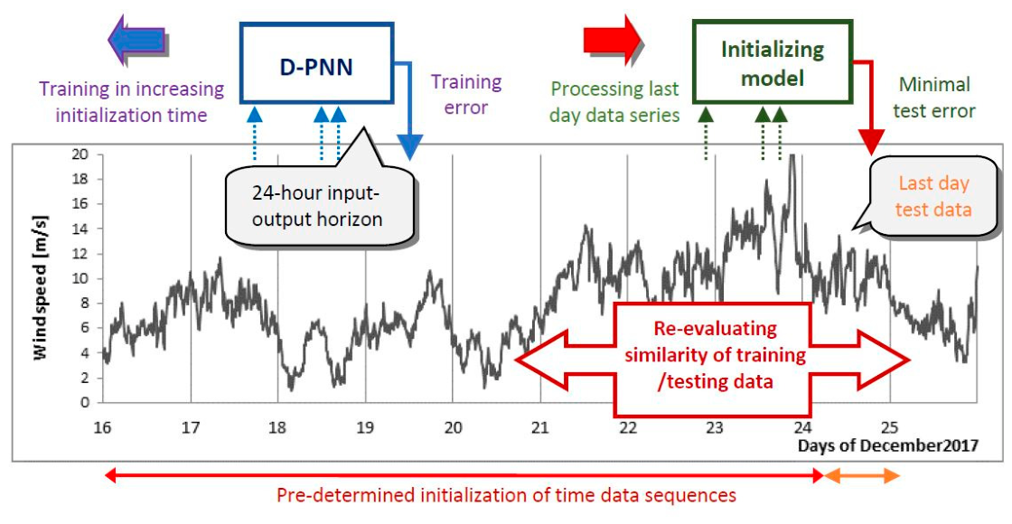
Figure 1 demonstrates the initialisation model search for the preliminary applicable day training intervals in the progressively increasing time points in each evaluation test in the latest data series. If examination models cannot obtain an acceptable approximation accuracy on the test data (in a case of overbreak), the start and end day points are moved in successive steps to find the appropriate initialising times for model training in the archive data set. The originally determined model day ranges were secondary reselected, evaluating each data record separately, according to the defined pattern similarity measure for the time counterparts at each testing hour [9].

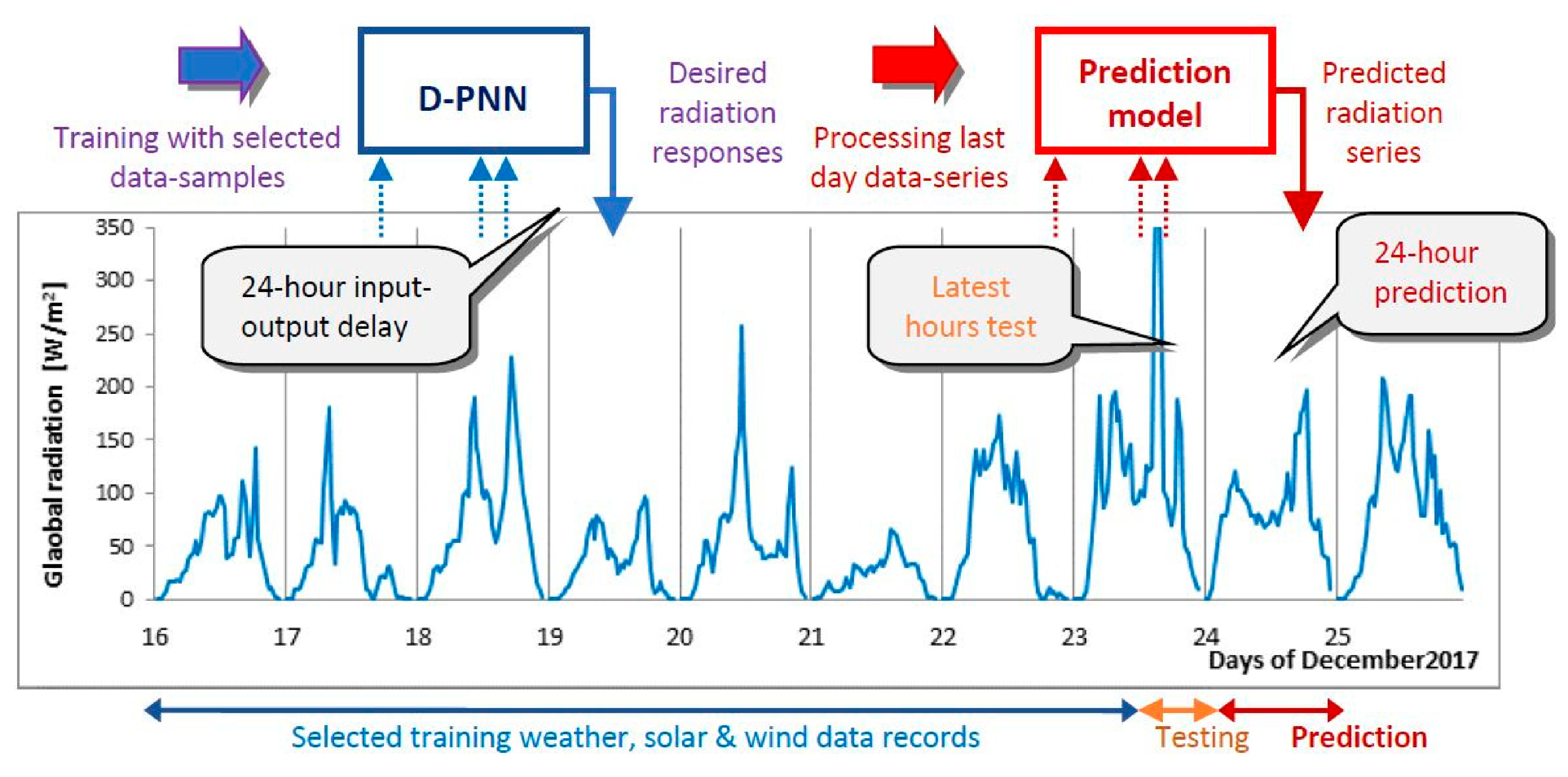
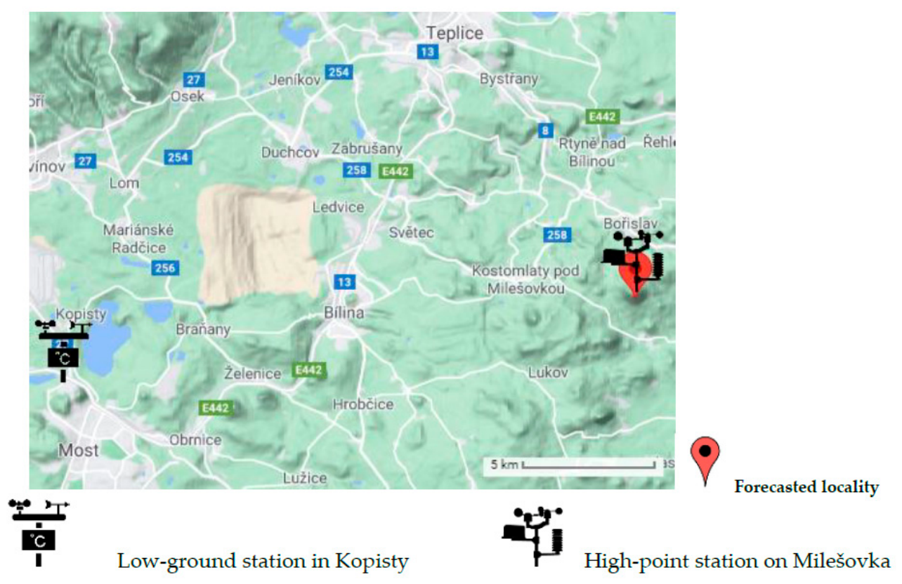
Figure 2 presents the self-determining training/testing procedure in modelling wind and solar ML output [28]. The completed models are finally tested on the last observation data to process an unseen input in computing approximate series in each response time of the target output in the next day series. If the developed models do not obtain a defined test threshold error, this indicates that the statistical prediction is not successful enough to be applicable in reliable RE day planning. Figure 3 shows a situation map of two professional weather facilities in low/high-level positioning [27].

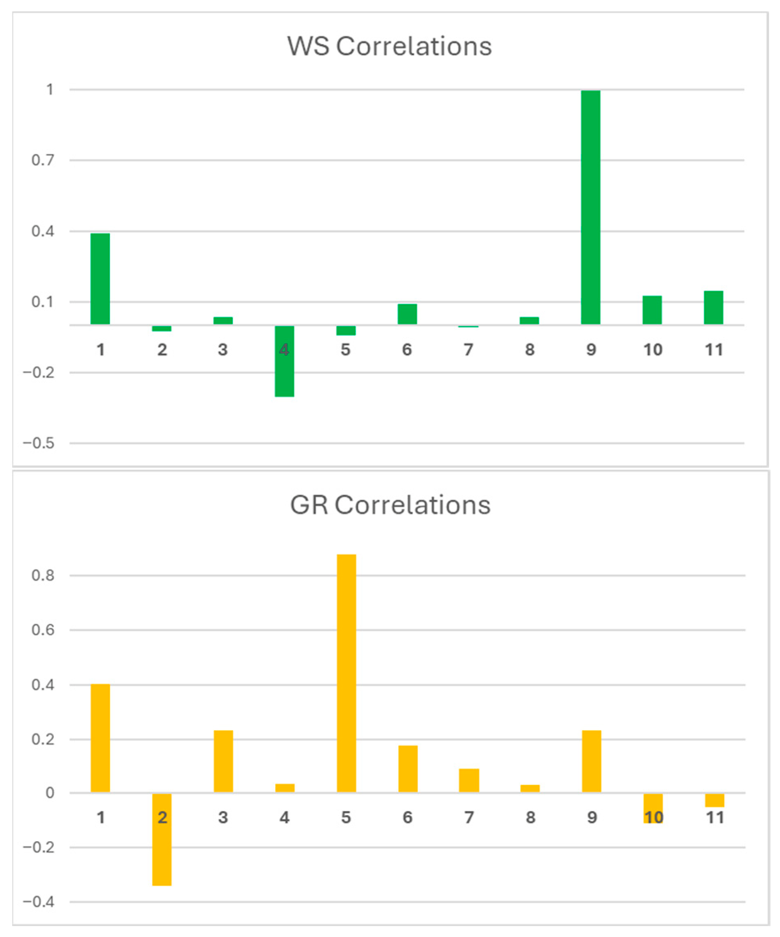
The correlation analysis between the relevant meteo-input and the WS/GR output is presented in Figure 4. Positive (+1) or negative (−1) degrees indicate a correlation type between two quantities. Positive (negative) type denotes the values in the first array are greater than 1, and the values in the second again are more than 1 (less than 1 or contrary). A degree value close to zero implies that there are no or only marginal data correlations [29].

4. Self-Optimising ML Methods in Wind-Solar Series Modelling

4.1. Differential Learning—A Novel Hybrid Neuro-Math Computing Approach

Differential Learning (DfL) is a new hybrid soft-computing approach, proposed by the author, which integrates adaptive evolutionary ML with numerical methods in solving partial differential equations. Differential Polynomial Neural Network (D-PNN) is a DfL-based regression technique that portions the general linear PDE of a kth order into reduced 2-variable PDE forms of a determined order (3) defined and L-converted in D-PNN nodes. DfL can model unknown nonlinear systems, described by a set of input variables, which are difficult to describe by conventional mathematical/physical equations or represent by conventional ML. The model evolution maximises the self-combination of optimal 2-input variables, without requiring data pre-processing in the initial stage. D-PNN evolves dynamically node-by-node a multilayer binomial tree structure, in each added or readapted layer. Each selected 2-combinatorial node forms a PDE-converted sum component, which is included (or extracted) in (or from) the overall model to iteratively improve the approximation of the target output. Step-by-step extension of the model usually yields optimal solutions based on Kurt Goedel’s incompleteness theorem. D-PNN nodes, connected in the backpropagation computing architecture, process 2-input data to pre-define and substitute their PDEs in the sum combinatorial model according to OC formulas. The polynomial node processing order evaluated for the component is directly correlated with the PDE transformation order [30]:

$$A{\displaystyle \frac{{\partial }^{2}u}{\partial x_1^2}}+B{\displaystyle \frac{{\partial }^{2}u}{\partial x_1{x}_2}}+C{\displaystyle \frac{{\partial }^{2}u}{\partial x_2^2}}+D{\displaystyle \frac{\partial u}{\partial x_1}}+E{\displaystyle \frac{\partial u}{\partial x_2}}+Fu=G$$

(3)

where A, B, …, G—parametric coefficient of x₁, x₂ independent variables of the unknown u function.

OC based conversion of nth-order derivatives describing an unknown f(t) function is formulated as the replacement Laplace transformation (L-transform) considering the known starting conditions (4):

$$L\left\{\left.f^{(n)}(t)\right\}\right.=p^{n}F(p)-{\displaystyle \sum _{k=1}^n{p}^{n-i}{f}_{0+}^{(i-1)}}\hspace{1em}L\left\{\left.f(t)\right\}\right.=F(p)$$

(4)

f(t), f′(t), …, f⁽ⁿ⁾(t)—continuous originals in <0+, ∞> p, t—complex and real variables, L—transform.

Derivatives in f(t) are L-converted to form algebraic Equation (5), where the images F(p) are separated in complex pure ratio forms (3):

$$F(p)={\displaystyle \frac{P(p)}{Q(p)}}={\displaystyle \frac{Bp+C}{p^2+ap+b}}={\displaystyle \sum _{k=1}^n\frac{A_k}{p-{\alpha }_k}}$$

(5)

B, C, A_k—coefficients of elementary fractions, a,b—polynom. Parameters, α₁, α₂, …, α_k—simple real roots.

The resulting ratio term represents the L-transforms F(p) of the original f(t) and can be restored by the inverse L-operation based on OC (6) to obtain the prime f(t) defined in a PDE (3) form:

$$F(p)={\displaystyle \frac{P(p)}{Q(p)}}={\displaystyle \sum _{k=1}^n\frac{P({\alpha }_k)}{Q_k({\alpha }_k)}}\cdot {\displaystyle \frac{1}{p-{\alpha }_k}}\hspace{1em}f(t)={\displaystyle \sum _{k=1}^n\frac{P({\alpha }_k)}{Q_k({\alpha }_k)}}{e}^{{\alpha }_k\cdot t}$$

(6)

P(p), Q(p)—multinomials of degree s−1, s, α₁, α₂, …, α_n—simple real roots of Q(p).

If f(t) is expected to be a separable function with regular time cycles determined by periods g_1,2,…,k, then its derivatives can be transformed into their sine and cosine counterparts. The original is again calculated by the inverse Laplace operation (7). This definition applies the amplitudes and phases of periodical data in obtaining the unknown periodical subfunctions from the node L images:

$$f(t)={\displaystyle \sum _{k=1}^r\frac{P({\alpha }_k)}{Q^{\prime }({\alpha }_k)}}{e}^{{\alpha }_k\cdot t}+2{\displaystyle \sum _{k=1}^s{e}^{{\beta }_k\cdot t}}(a_k\cdot \cos {\gamma }_{k}t-b_k\cdot \sin {\gamma }_{k}t)$$

(7)

β₁, β_2m, …, β_n—imaginary roots of Q(p).

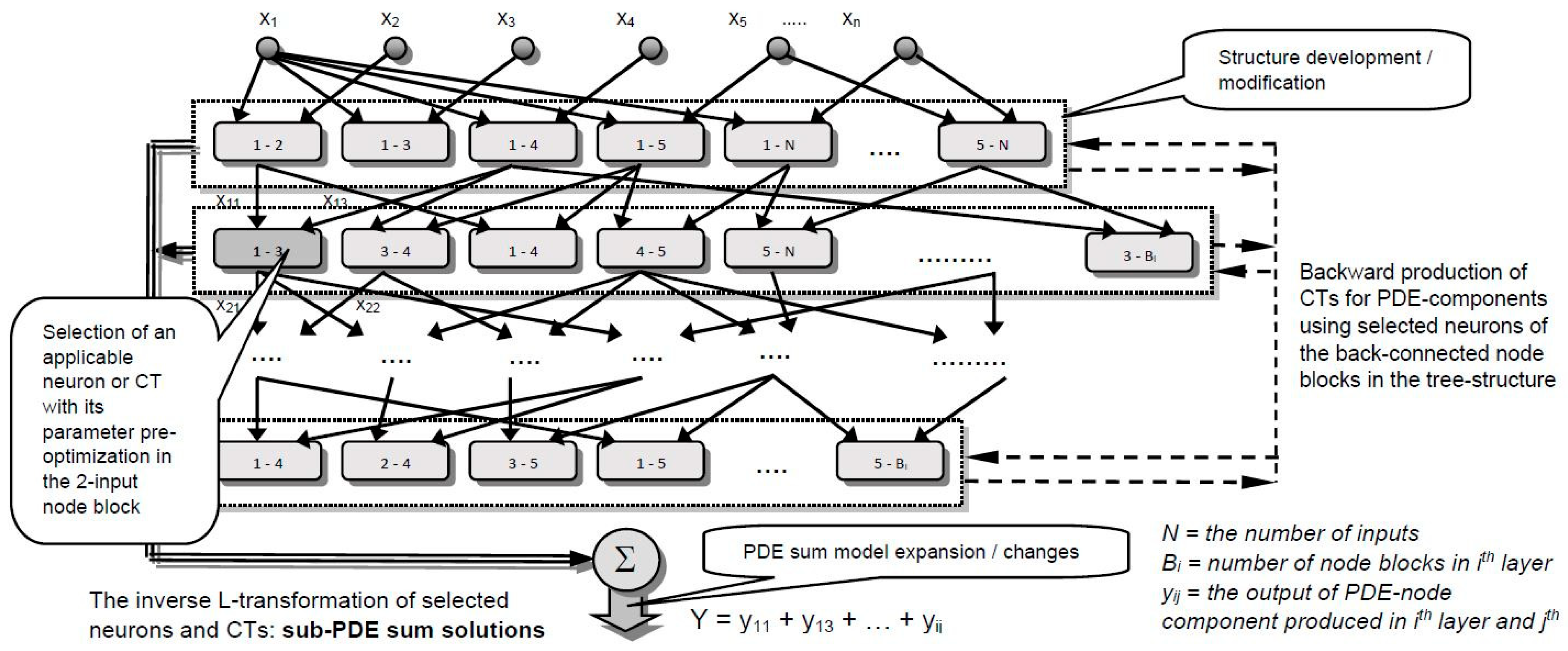
Inverse recovery is applied to the rational (6) or periodic L-image PDE terms (7), obtained by the initial conversion. Original u_k produced in D-PNN node blocks (Figure 5) is summed in the modular output of a PDE model in approximation of the unknown n-input u function (3).

The inverse operation applied to the expressed F(p) ratio of an analogously converted node PDE (6) is represented by the angle exponent f = arctg(x₂/x₁). The real 2-variable form of y(x₁, x₂) is restored from an L-transformed ratio (8) to obtain the fractional solution of the y_j PDE node (3):

$$y_1=w_1{\displaystyle \frac{b_0+b_1{x}_1+b_{2}sig\left(x_1^2\right)+b_3{x}_2+b_{4}sig\left(x_2^2\right)}{a_0+a_1{x}_1+a_2{x}_2+a_3{x}_1{x}_2+a_{4}sig\left(x_1^2\right)+a_{5}sig\left(x_2^2\right)}}\cdot e^{\varphi }$$

(8)

y_j—partial sub-PDE solutions of node u_k functions, sig—sigmoidal transformation.

• φ = arctg(x₂/x₁)—angle of 2-input variables x₁, x₂, a_i, b_i, w_j—polynom. parameters and term weights.

The periodic conversion of a PDE node with the doubled input x₁, x₂ and γ₁, γ₂ (9) is derived from (7):

y_i = [a₁x₁ × cos(b₁2π.γ₁.t + b₀) − a₂x₂. sin(b₂2π.γ₂.t + b₀)] × e^ϕ

(9)

y_i—periodical output of a node PDE-term, γ₁, γ₂—phases [radian], x₁, x₂—real amplitudes, a, b—coeff.

Data time t periods can be represented by Fourier series in converted node PDEs considering their derivatives (10):

Y_i = [a₁x₁. cos(b₁π.t + b₀) + a₂x₂. sin(b₂π.t + b₀)] × e^ϕ

(10)

y_i—Fourier representation of a node PDE-term for t—time, x₁, x₂—amplitude variables, φ = γ₂ − γ₁.

The terms of the imaginary Euler number c (11) are related to the formulation OC based on the exponential function (6), The radius r (amplitude) can replace the rational component for the phase (frequency) φ = arctg(x₂/x₁) for the variables x₁, x₂ related to the inverse transform of F(p):

$$c=\underset{\mathrm{Re}}{\underbrace{x_1}}+i\cdot \underset{\mathrm{Im}}{\underbrace{x_2}}=\sqrt{x_1^2+x_2^2}\cdot e^{i\cdot \arctan \left({\displaystyle \frac{x_2}{x_1}}\right)}=r\cdot e^{i\cdot \varphi }=r\cdot (\cos \varphi +i\cdot \sin \varphi )$$

(11)

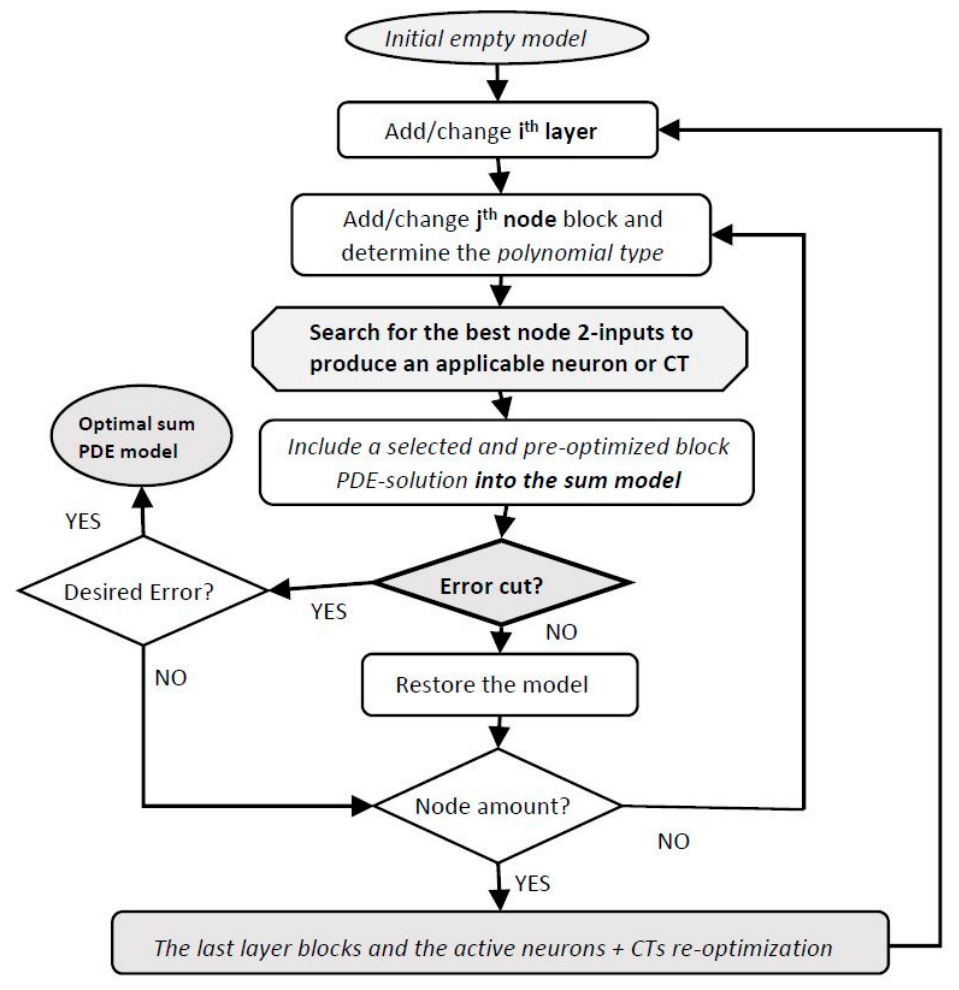
Figure 5 presents the backward production of PDE node components in a tree multilayer node structure. Synchronised 3-level optimisation algorithms are used in D-PNN model development, starting empty, adding/revising node by node in each evaluated layer of a growing binomial tree backward structure producing applicable node PDE components (see flow chart in Figure 6).

Characteristics of D-PNN models [29]:

▪

Splitting the n-variable general-order PDE into a defined set of reduced PDE converts

▪

Developing PNN structures by inserting node by node into the back-computing structure

▪

Producing PDE components in each added PNN node to be involved in the sum model.

▪

Several types of PDE conversions using OC base functions to define its computing frame

▪

Using L-transforms of PDE-derivatives and the inverse OC recovering of node originals

▪

(Re)selecting dynamically optimal 2-inputs to expand the parallel PDE-component model

▪

Non-downsizing significantly data dimensionality leading to an over-reduction in models

▪

Various combinations of model components are selected.

4.2. Deep Learning with Matlab DL-Toolbox

DL is an efficient computing approach capable of learning long-term patterns from input–output samples, using a complex architecture design of several structural layers, without relying on the progressive development model. The Matlab DL Toolbox (DLT) is a framework that comprises quick design, parametric, and training settings of deep neural networks. DLT offers long-short-term memory (LSTM) networks using sequence-to-sequence regression [31], whose basic structure usually consists of the following levels:

○

Input-sequenced layer

○

LSTM layer

○

2nd processing layer-fully-connected

○

Drop-out layers

○

1st processing layer-fully-connected

○

Output-regression layer

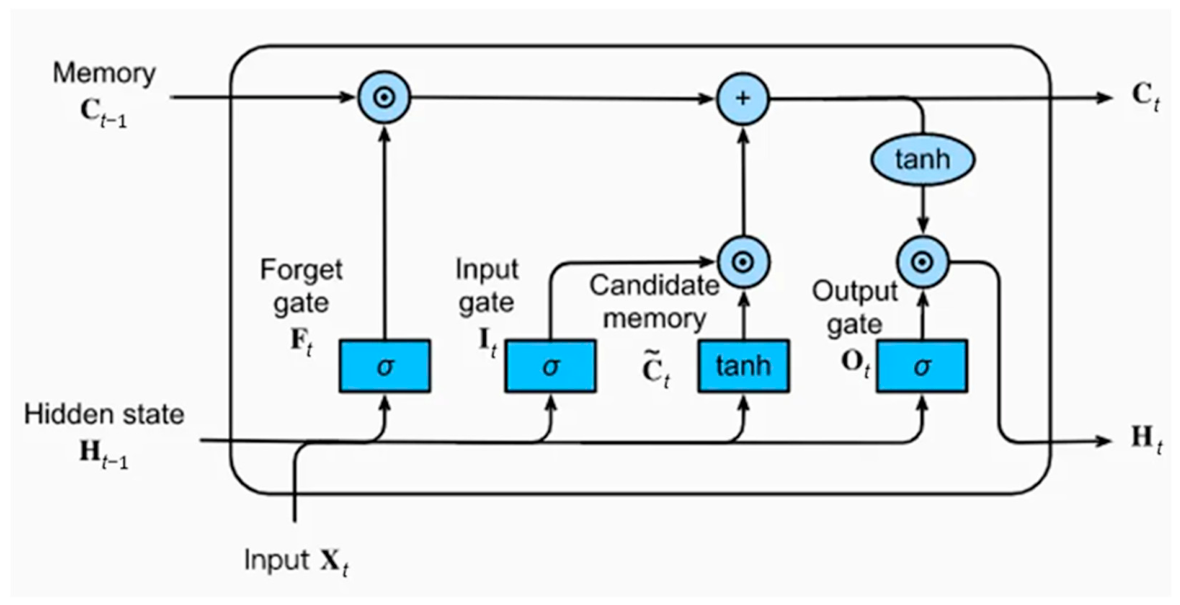
The master part of the DL-based regression is the key LSTM layer. An input sequence layer supplies data series to the network structure. The LSTM layer processes input sequences to capture long-term data patterns in defined time steps. The output is represented by hidden H_t states and C_t cell C_t states. Time-delayed LSTM blocks compute the current and hidden states (C_t−1, H_t−1) to be integrated with the input vector in the next computation step of the H_t output, representing an inner state to update the cell C_t state at each time t (Figure 7). LSTM layers keep information from previous times, t − 1, t − 2, etc., applied in the next recurrent updates. A dropout layer sets random inputs to zero values according to a probability distribution function to reduce overfitting. The loss of gradient functions is applied for the minimum predefined batch length in several data subsets to optimise input weight updates in training [32].

The forget gate (12) decides which information to keep and which to forget, applying sigmoid activation to the weights W_f multiplied by the concatenated previous hidden state H_t−1 and the current input X_t, plus the bias b_f:

F_t = σ (W_fZ_t + b_f)

(12)

Candidate gate memory (13) processes new information Z_t = H_t−1. Xt which is computed in the LSTM layer and multiplied by the weights and biases W_c and b_c in hyperbolic tangent activation:

C_t = tanh (W_cZ_t + b_c)

(13)

The input gate (14) analogously to (9) decides which information supplied to the network is remembered in the opposite of the memory state:

I_t = σ (W_iZ_t + b_i)

(14)

The output gate (15) again determines what information to remember between the 2-hidden states by the sum of bias b_o and the product of the weights W_o and the concatenated input Zt:

O_t = σ (W_oZ_t + b_o)

(15)

The final gate (16) usually does not regularly contain an activation function applied to the H_t output, although it may be useful in some applications:

Y_t = W_yHS_t + b_y

(16)

DLT is based on the well-known basic LSTM architecture able to learn complex correlations from input–output samples. This complex hybrid recurrent network type can integrate multiple processing (in simple computing elements) with biologically inspired operation based on connection gates. DLT networks require primarily a hand-design for a defined layer-replicate structure, which may also comprise different layer types [33]. LSTM retains a hidden state H_t with an extra memory cell state C_t. This inner type of cell memory allows the retention of information from long-term patterns, while hidden states usually hold short-term relationships learnt from data (Figure 7).

4.3. Machine Learning Regression with Matlab Statistics Toolbox

The Matlab Statistics and ML Tool-Box (SMLT) methods were applied in evaluation of the models evolved in data-driven predicting WS and GR. SMLT offers a variety of novel neurocomputing, aggregative stochastic, or conventional mathematical ML methods [34]:

• Linear interaction, stepwise, and robust regressions apply simplified parametrised equations, easily adaptable and interpretable in the processing of input data.
• Fine, medium, and coarse regression trees progressively evolve binary branch structures that are easy to interpret and fit to data samples in iterative training. Initialising the root starts with processing data input in developing branches that reach the terminal leaves according to identified predictor states. Inputs are evaluated on the binary nodes to determine the optimal way to be applied in the next decision step. The output of terminal leaves corresponds to the overall response of a model. Fine trees contain a higher amount of node branches/leaves, which detail the problem representation and usually have less generalisation ability on testing samples of unknown data. They often suffer from overfitting, which means substantially lower accuracy compared to those of training. Coarse trees on the other side are built from a smaller number of large leaves, which does not allow high accuracy in training but yields robustness in processing unseen data input in validation. It is necessary to optimise and balance tree development between the two borderline schemes.
• The Support Vector Machine (SVM) is based on computing linear, cubic, square, Gaussian, or Radial Basis Function (RBF) kernels obtained from the defined input data transformation, first applied before the ML process. The linear ε training parameters eliminate/ignore output errors, outside of the interval ε vector, if they are assumed to be zero/‘1’. The support vectors represent the output delimiting intervals where errors exceed the defined ε values.
• Gaussian Processed Regression (GPR) is used in a space of problem definition for a determined probability distribution in calculating the output according to the linear, constant, or zero-base functions, supplied as a prior GPR model. Rational, exponent, square exponential, quadratic, or maternal kernel functions define a distance space vector in each predictor evaluation in the model output response.
• Aggregation trees: Ensemble-Boosted/Bagged (EBT, EBoosT/EBaggT) produce ensemble weighted outputs for a set of week-learner tree models. The least squares strategy of bagging, boosting, and bootstrapping in data sampling is applied in model training to compose and ensemble based on probabilistic statistics (Section 2).

Principal component analysis (PCA) of an additional SMLT item was applied before ML but without improving the WS- and GR-day forecasting in processing the selected data input. Forecasting models are finally validated on the last available data samples, and those obtaining the best approximation accuracy are used to calculate day-ahead series.

5. ML Experiments in Data-Driven Day Wind and Solar Prediction

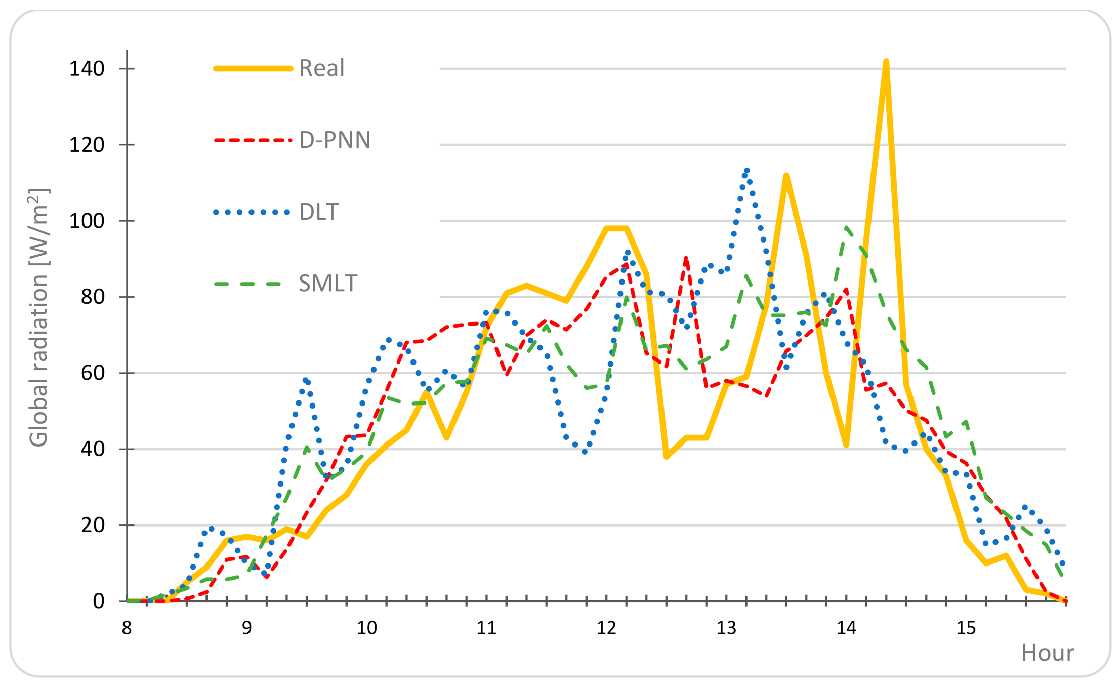
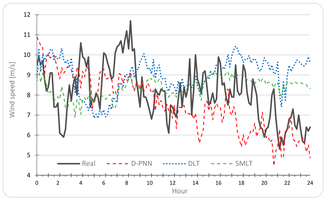
The meteo-data sets from 2-layer low/high base stations (Figure 3) were used in the wind/solar prediction experiments and the evaluation of two groups of manifold ML self-optimising models, using the described point-time initialisation and training data re-evaluation in preprocessing (Section 3). If the pattern similarity (2) between input samples, comprised in the initially pre-assessed interval (Figure 1), and the related last observation time-referenced series is above the defined correlation threshold (0.5), the samples are included in the final training set. An extensive search for several initialisation times may be performed on the available data in the case of impracticability of the determined learning samples. D-PNN automatically searches for the optimal 2-input nodes in the structural models to obtain an initial list of high-scored PDE components, separately examined to be possibly included in the output sum. Self-organising structures are formed in the node by adaptive learning of D-PNN and SMLT. The D-PNN models are complementary tested and finally verified to be applied to unknown next-day input to compute 24/8 h shifted output series. This one-stage day-flush data processing considerably reduces computational costs and procedural complexity by applying one prediction model to the latest input for each reference time output. The best prediction model is chosen from various runs using random or user-adaptive start-ups, according to the lowest testing errors in the last hours. Figure 8 and Figure 9 demonstrate the character of real-world and prediction output series in the secondary data delay experiments in the ranges: 0–24 h for wind speed and 8–16 h for radiation, obtained by PDE-transformative D-PNN, recurrent DLT, and probabilistic SMLT models in the monitored 10-day autumn–winter period.

All evaluated ML models are commonly successful in approximating sudden variances in the target GR or WS series under partly unsettled environment conditions (Figure 8 and Figure 9). The D-PNN models mostly better reflect rapid dynamical time changes in the next-day pattern progress. The WS and GR character of day cycles is mostly stable, as shown in the illustrative graphs, but an essential night change from 21 to 22 December and in the following period (Figure 1 and Figure 2) becomes evident with gust and cloud conditions. The solar series were first transformed to relative CSI to avoid absolute day-alteration data resulting from the actual solar intensity and horizon level. CSI data are normalised by considering maximal clear-sky GR values to eliminate seasonal effects. The computed GR output is renormalised from the nominal CSI series to restore the target output [8]. Periodical and angular data (GR, temperature, wind azimuth, etc.) are self-detected by D-PNN to be related to the amplitude time in day cycles in the PDE conversion using the L transform functions (sine, cosine) (7). SMLT methods use a self-optimising framework (analogous to D-PNN) without a mandatory trial–error design in training hyperparameters or layer structure (as DLT requires).

6. Evaluation of ML Results in Wind and Solar Day Prediction

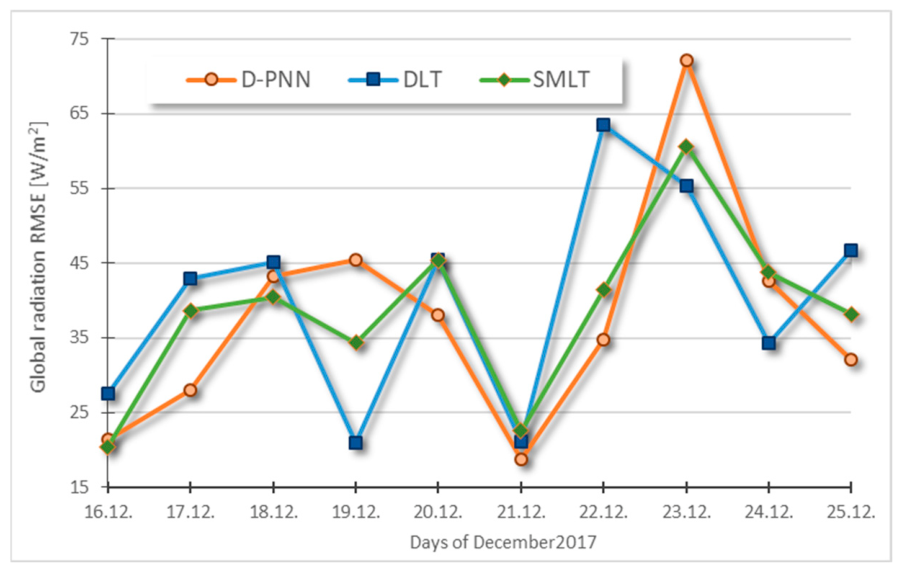
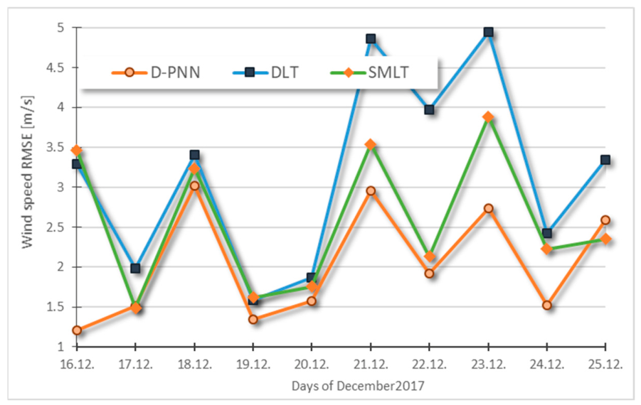
The model hourly-average errors are summarised in the day-interval ML predictive results in the wind and solar approximate series in the statistically examined 10-day autumn–winter period (Figure 10 and Figure 11). A significant over-change period in wind patterns (gust and blast) from December 21 (Figure 1) brings on accumulative errors of all models (Figure 9). A notable fall in GR on the same day and its pattern turnover from 22 December (Figure 2) project analogically to a predictive debase in model output of the successful ML techniques in the next days (Figure 11). This type of overbreak error in prediction can be reduced by an algorithmically widespread search for applicable training samples (2), if extensive tabular data archives are accessible.

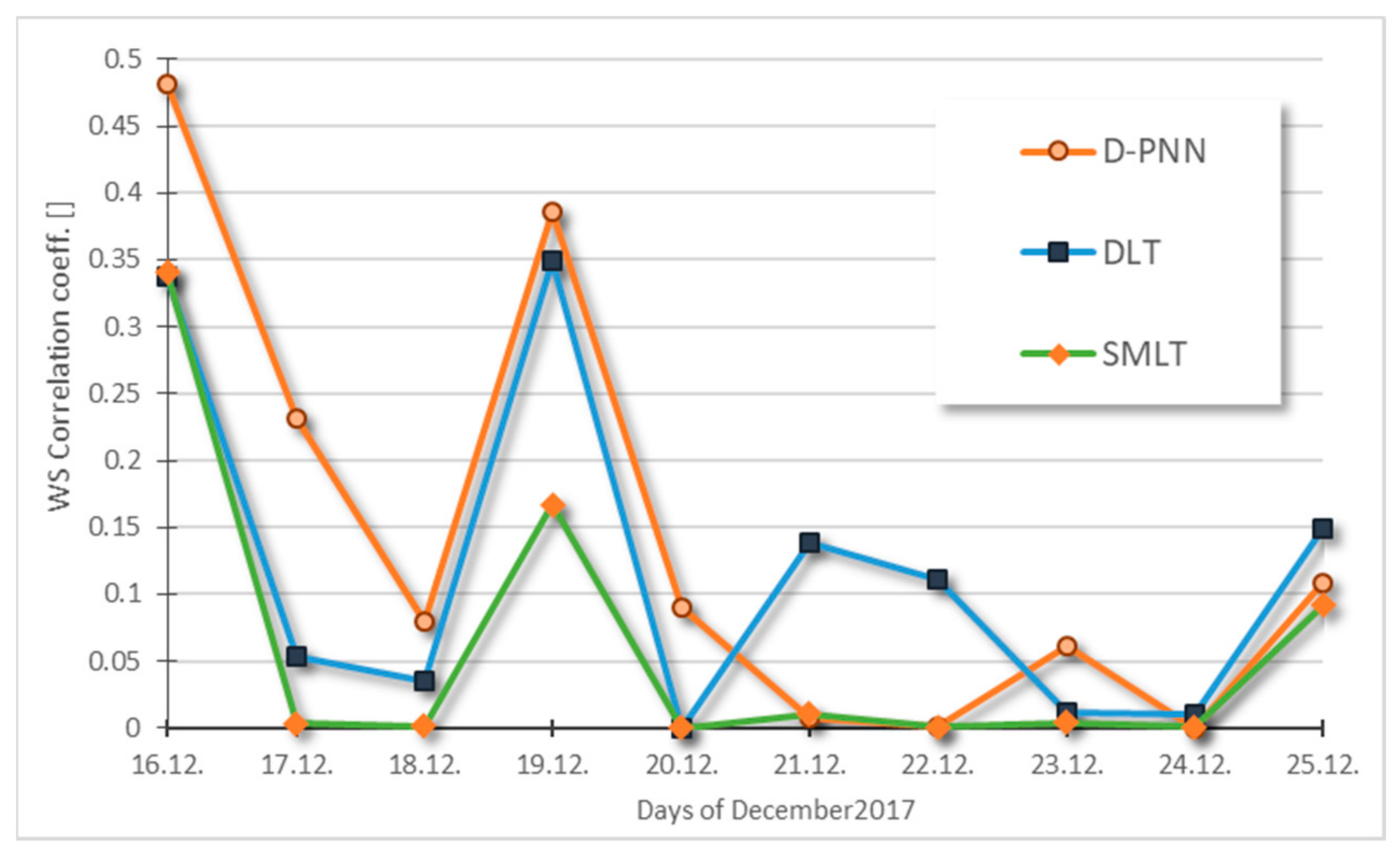
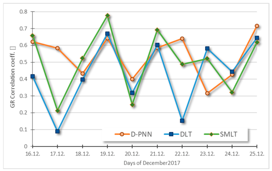
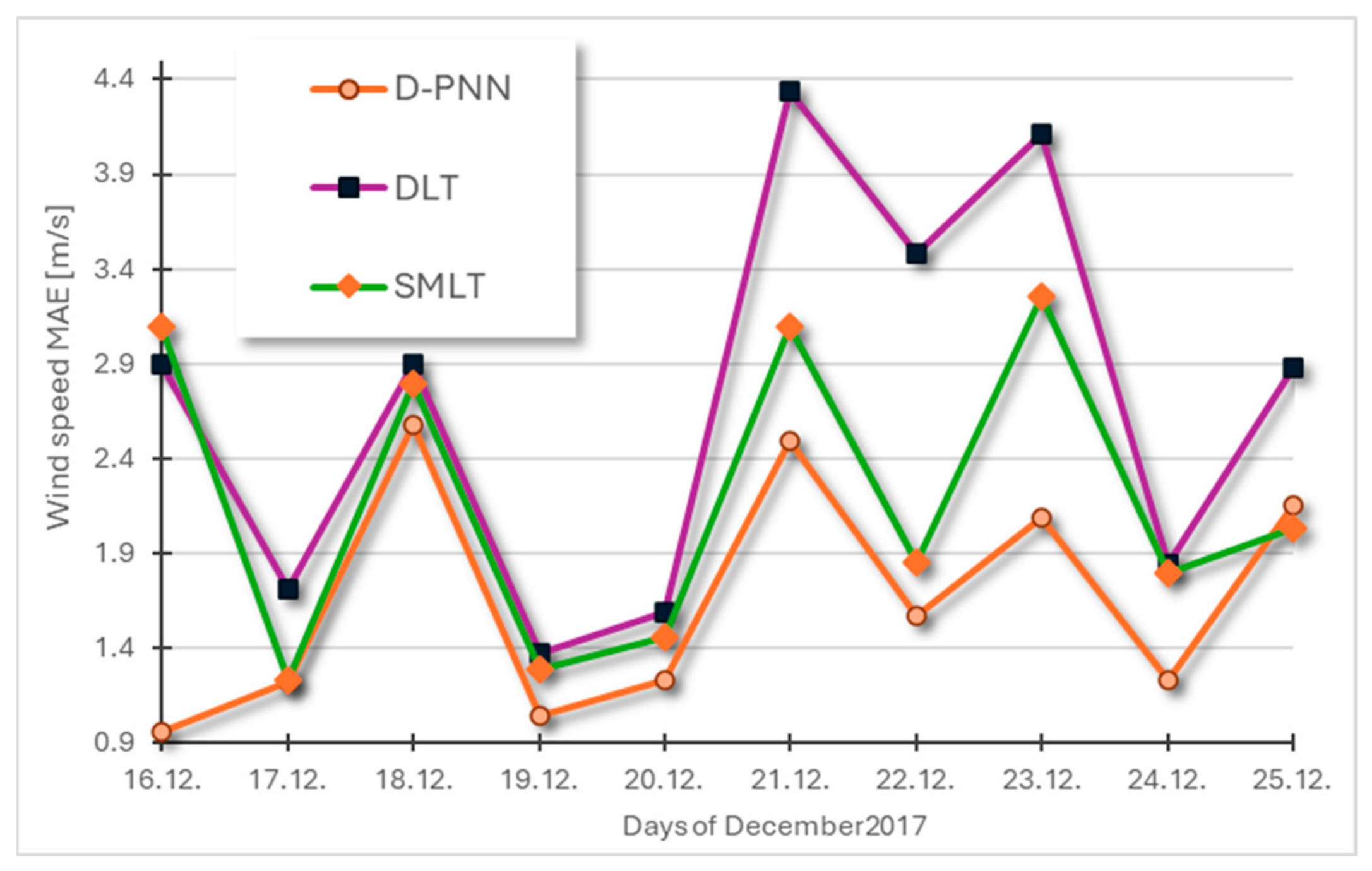
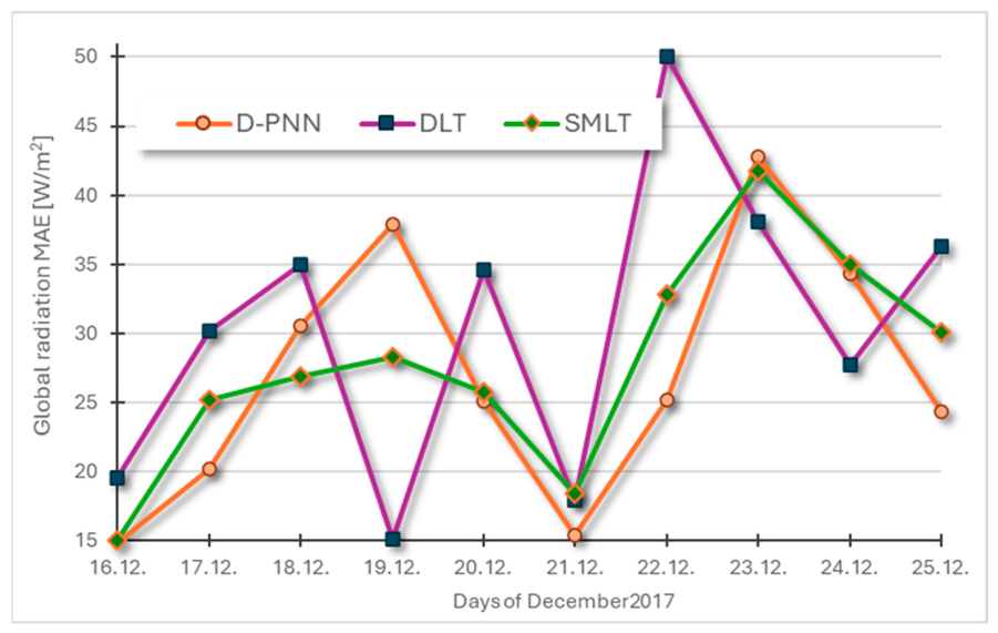
The approximation accuracy of data-driven ML models is predominantly affected by the initial selective processing of optimal training samples [8]. Pearson‘s correlation coefficients R² are calculated for each prediction model (Figure 12 and Figure 13) to compare statistical precision in 10-day experiments. A notable drop in all-say predictive R² values in the SMLT output implies an undesired WS averaging using GPR probabilistic and EBT distributive modelling in the second half period (Figure 8). The overall results of the most successful ML models differ slightly in 8 h GR and partially in 24 h WS estimations. The daily WS approximation has only small variances in precision. The complex D-PNN modular concept mainly outperform DLT and SMLT in predicting unstable WS and mid-in cycle GR series. All compared ML methods get better day-ahead accuracy in approximating irregular GR daily periods than chaotic WS variations. More diverse spatial/multilevel observational data would naturally improve pattern representation and reliability in early model development and predictive computing in eliminating unexpected failures. The graphs in Figure 14 and Figure 15 present the mean absolute error (MAE) in the predicted WS/GR series, whose day points show correlations with the RMSE progress.

WS was predicted 24 h ahead each 10 min, while GR day cycles were approximated by 8 h prediction series in 30 min intervals, which is sufficient with respect to daylight periods and lower time variability in the cloud progress (demonstrative Figure 8 and Figure 9). Thus, the quality of WS 24 h approximate series in a detailed 10 min average interval is naturally lower than the GR 30 min estimation. In addition, GR shows a stronger correlation degree between input–output series (Figure 4), which gives it advantages over WS in modelling using ML. The predictive WS coefficients of R² (Figure 11) are abnormally low, mainly in the second half of the evaluated period, probably due to an increase in the instability of complex wind factors under changing conditions. Chaotic variability and dust uncertainty in wind series, whose rapid changes are difficult to adequately approximate 24 h ahead, also debase predictability (Figure 8).

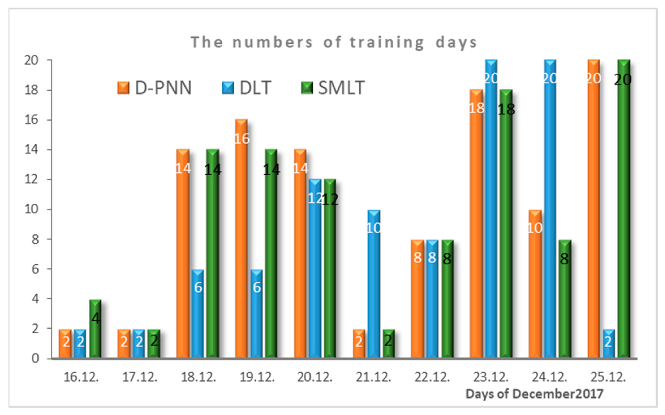
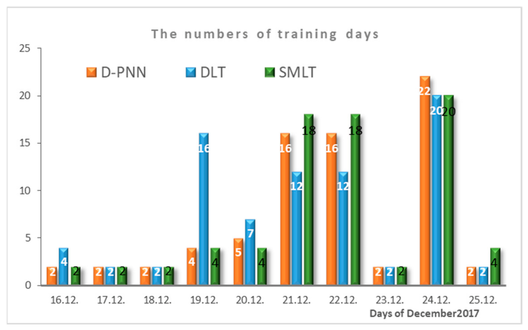
The detected primary modelling initial daytime points (Figure 16 and Figure 17) are re-evaluated in the secondary similarity distance search of the optimal training row data.

The computed output of all evaluated ML models is significantly correlated, which denotes analogical data preprocessing and training. The PDE-modular concept of DfL levels with the best approximation of target series in each prediction day (Figure 10 and Figure 11), although a slightly inferior performance in a few cases. Models were developed with analogical day initialisation times (Figure 16 and Figure 17), except DLT, which required an extension in the day sample intervals under overnight breaks in conditions. DLT needs more detailed recognition of day-training intervals (Section 3) and eventual extended search for additional data time points, as compared to the more resistant probabilistic and PDE-component model forms producing reliable 24 h prognoses. D-PNN models are limited by the exponentially increasing combinatorial variants evaluated in an extensive search for optimal input, although the manifold of PDE solutions adequately reflects the uncertainty in atmosphere progress. Error day alterations result from unexpected environmental changes, where D-PNN proved its robustness compared to DLT or SMLT (Figure 8 and Figure 9). The DfL data transformation contributes to a more stable model output. The best SMLT models are GPR and EBT based on probabilistic and distribution statistics (Section 2). The proportion of models chosen was 7:3 (GPR vs. EBT) in WS and 5:5 in GR. The stochastic nature of GPR and the aggregate EBT of SMLT [34] was found to be efficient in the approximation of the GR cycle series using denormalised CSI output (Figure 9). Their prediction in WS in some days can result in averaging output at some times, which is denoted by a drop in the R² correlation coefficient (Figure 12).

7. Discussion

Rapid changes in training and prediction data patterns are usually the result of surface irregularity interactions in air flow circulation and chaotic instabilities in conditions. These uncertain states cause training difficulties and impracticability in computing 24 h shifted output related to the model input. The approximation of ramping series requires selective data searching to optimise learning in adaption to the current patterns progresses. Short-term instabilities induce abrupt oscillations in WS or GR (Figure 8 and Figure 9) that are hardly predicable behind a few hour horizon. The optimal extraction of training samples depends on the evaluation strategy in pattern similarity (correlation distance between two input vectors) (2). A more complex measure could improve selective training. A more complex comparative measure for each evaluated input–output sample could be used in a short time-range of series (6 h) in selective training. Data-driven ML predictions mostly fail after unexpected breaks in overnight weather development. The characteristics of WS or GR data in training and forecasting time may be entirely uncorrelated in abrupt frontal interference. A defined validation threshold can be used in reference to previous-day failures or NWP data in computing series. If the output of an ML model is not within an error limit, a transformative NWP forecast can be used instead. Previous abnormal changes in data patterns can be searched and revealed retrospectively in data archives to reassess optimal model initialisation times (Figure 11). An extra 24 h delay in the input of day-cycle data can be supplied to the model (humidity, radiation, power load, etc.) to improve data-driven ML.

8. Computing Limits and Research Perspectives

The predominant training intervals improve the approximative statistics of self-contained models, which are unable to simulate all-over atmosphere dynamics on a midscale. Recognition of optimal learning samples requires extra searching time in scanning large observational archives, though training is simplified to a sequential procedure. Examination of pattern similarity with respect to NWP could improve data sampling in model initialisation. NWP tabular archives [28] are not freely available compared to easily accessible historical databases [27]. The D-PNN optimalisation costs are evidently higher as a common elaborated Matlab ML, as it faces extensive combinatorial expansion. Stepwise DfL binary optimisation was found to be efficient in modelling unknown dynamical systems. The D-PNN input is limited to dozens of quantities to compute the output in a foreseeable time; thus, processing high-dimensional data is not effective. Lagged input improves model quality, although it requires extra processing time. Parameters initialisation and heuristic strategies minimise additional time in combinatorial search for backward-optimised node PDE components. Added or removed PDE components included in the output model can be readapted within the new data set. Incremental training improves the previously acquired modelling capabilities to process different inputs. The complexity of D-PNN structures is proportional to the patterns learnt from additional input–output samples [30].

9. Conclusions

CD sampling in data-driven GR/WS modelling was experimentally validated using advanced PDE-modular, deep neural, and soft computing day-predictive self-optimising ML approaches. Iterative day-sequence computing implemented on a fixed time horizon proved its effectiveness in time reduction and early access. The presented statistical learning allows for on-time prediction of 24 h output series in high-speed procedure competing intraday ML or NWP based approaches. Differenced-data relationships allow for modelling pattern progression in higher time frames than usual in ML. Similarity-based selective training improves model stability and reliability in computing chaotic WS and alterative day GR cycles. The solid DfL modular concept proved its ability to reflect rapid dynamical changes and progress in prediction times. It mostly overcomes regular Matlab ML in approximating target series, despite some unsolved optimisation questions. The early-supplied GR/WS prognoses help plan the utilisation of RE facilities on a daily basis. Physical NWP simulations better reflect irregular breaks in air circulation, despite a significant delay in their delivery and accessibility. ML day models rely purely on training statistics, which require optimising data sampling, especially in doubtful cases. An early warning system that uses NWP utilities in pattern analysis can eliminate self-standing ML predictability flaws. Intra-hourly ML models in reduced time usually correct the first overall prognoses obtained in the effective day-sequence procedure. Inconsistent output produced by flawed ML models should be revealed as a discrepancy in learning and representing real pattern progress in forward testing. Parametric C++ software, observational wind radiation, and additional quantity data sets are available in public repositories for comparative verification experiments [29].

References

1. Sohan, F.A.A.; Uddin, H.; Kumar, L.; Nahar, A.; Rudro, R.A.M. Forecasting solar photovoltaic power generation: A machine learning time series model approach. Int. J. Energy Res. 2025, 15, 4092367. [Google Scholar]
2. De Santis Alessio Verdone, E.; Panella, M.; Rizzi, A. A review of solar and wind energy forecasting: From single-site to multi-site paradigm. Appl. Energy 2025, 392, 126016. [Google Scholar] [CrossRef] [Scilit]
3. Giannopoulos, A.; Karditsa, A.; Hatzaki, M.; Trakadas, P. Machine learning for wind pattern estimation at data-scarce coastal ports: A comparative study using real measurements. J. Mar. Sci. Eng. 2025, 13, 2375. [Google Scholar] [CrossRef] [Scilit]
4. Almuzakki, M.Z.; Ramadhan, H.; Akhir, E.A.P.; Yunita, A.; Pratama, I. Performance analysis of neural network architectures for time series forecasting: A comparative study of rnn, lstm, gru, and hybrid models. MethodsX 2025, 15, 103462. [Google Scholar] [CrossRef] [Scilit]
5. Song, W.; Zhang, H.; Wang, H.; Ge, C.; Yan, J.; Li, Y. Middle-term wind power forecasting method based on long-span nwp and microscale terrain fusion correction. Renew. Energy 2025, 240, 122123. [Google Scholar]
6. Tai, N.; Liu, S.; Pu, C.; Fan, F.; Yu, J. A hybrid strategy for probabilistic forecasting and trading of aggregated wind-solar power: Design and analysis in heftcom2024. Int. J. Forecast. 2026, in press. [Google Scholar]
7. Jiang, M.; Zhu, S.; Zhang, H.; Zhang, D.; Chen, D.; Shi, X.; Chen, Y. Selecting effective nwp integration approaches for pv power forecasting with deep learning. Sol. Energy 2025, 101, 1–17. [Google Scholar]
8. Pechlivanoglou, G.; Bianchini, A.; Superchi, F.; Moustakis, A. Can machine learning enhance day-ahead renewable power forecasts? A study on data-driven methods for solar photovoltaic and wind turbines. Energy 2025, 336, 138396. [Google Scholar]
9. Mo, X.; Huang, G.; Li, H. A novel point-interval prediction model for wind speed based on hybrid deep learning and rime optimization algorithms. Energy Rep. 2023, 14, 3977–3992. [Google Scholar]
10. Gupta, A.K.; Singh, R.K. A review of the state of the art in solar photovoltaic output power forecasting using data-driven models. Electr. Eng. 2025, 107, 4727–4770. [Google Scholar] [CrossRef] [Scilit]
11. Karthikeyan, V.; Karthick, A.; Sathiyaseelan, V.; Selvaraj, J.; Muthuramalingam, L. Optimizing wind energy integration: A review of forecasting techniques and emerging trends. Arch. Comput. Methods Eng. 2025, 33, 4261–4286. [Google Scholar] [CrossRef] [Scilit]
12. Wang, H.; Ge, C.; Liu, Y.; Yan, J.; Han, X. An ai-based weather prediction method for wind farms combining global forecast field and wind speed temporal transfer characteristics. Energy 2025, 329, 136740. [Google Scholar] [CrossRef] [Scilit]
13. Abdulkader, H.M.; Mohammed, A.M.; Attya, M.; Abo-Seida, O.M. A hybrid deep learning framework for solar irradiation prediction based on regional satellite images and data. Neural Comput. Appl. 2025, 37, 14327–14363. [Google Scholar] [CrossRef] [Scilit]
14. Mohanasundaram, V.; Rangaswamy, B. Photovoltaic solar energy prediction using the seasonal-trend decomposition layer and asoa optimized lstm neural network model. Sci. Rep. 2025, 15, 4032. [Google Scholar] [CrossRef] [Scilit]
15. Su, J.; Yang, Y.; Chen, Y.; Hu, X.; Sun, P.; Ding, T. A fine-grained frequency decomposition framework for long-term photovoltaic and wind power forecasting. Sol. Energy 2025, 301, 113930. [Google Scholar]
16. Salem, F.M. Recurrent Neural Networks; Textbook; Springer: New York, NY, USA, 2022. [Google Scholar]
17. Pereira, S.; Canhoto, P.; Oozeki, T.; Salgado, R. Comprehensive approach to photovoltaic power forecasting using numerical weather prediction data and physics-based models and data-driven techniques. Renew. Energy 2024, 251, 123495. [Google Scholar] [CrossRef] [Scilit]
18. Yan, Z.; Wu, L.; Qiu, R.; Zhao, S.; Qiu, Y.; Luo, Y. The potential of ai global weather models for reference evapotranspiration forecasting: A comparison with numerical weather prediction models. J. Hydrol. 2026, 664, 134363. [Google Scholar]
19. Tahir, M.; Zhang, Y.; Bashir, T.; Wang, H. Wind and solar power forecasting based on hybrid cnn-abilstm, cnn-transformer-mlp models. Renew. Energy 2025, 239, 122055. [Google Scholar]
20. Shan, S.; Li, C.; Wang, Y.; Zhang, K.; Wei, H.; Dou, W.; Wang, K.; Sreeram, V. Day-ahead numerical weather prediction solar irradiance correction using a clustering method based on weather conditions. Appl. Energy 2024, 365, 123239. [Google Scholar] [CrossRef] [Scilit]
21. Cheng, P.; Chen, X.; Han, T.; Da, X. A novel interval prediction method in wind speed based on deep learning and combination prediction. Sci. Rep. 2023, 15, 23182. [Google Scholar] [CrossRef] [Scilit]
22. Yang, J.; Niu, M. Wavegru: A framework with frequency-domain spatial attention for accurate solar pv and wind power forecasting. Sustain. Energy Technol. Assess. 2025, 83, 104572. [Google Scholar] [CrossRef] [Scilit]
23. Zhou, Y.; Wang, J.; Zhang, Y.; Xu, C. Optimal operation of wind-solar-storage-hydrogen system considering multi-scale forecasting of source-load. Energy Convers. Manag. 2025, 344, 120296. [Google Scholar]
24. Ye, J.; Zheng, L.; Wu, Y.; Wu, Y. Optimizing meteorological predictions to improve photovoltaic power generation in coastal areas. Sustain. Energy Technol. Assess. 2025, 78, 104345. [Google Scholar]
25. Meng, Z.; Guo, Y.; Zhao, C. Probabilistic wind power forecasting with missing data tolerance: An end-to-end nonparametric approach. IEEE Trans. Sustain. Energy 2025, 17, 1202–1213. [Google Scholar] [CrossRef] [Scilit]
26. Zjavka, L. Power quality 24-hour prediction using differential, deep and statistics machine learning based on weather data in an off-grid. J. Frankl. Inst. 2023, 360, 13712–13736. [Google Scholar] [CrossRef] [Scilit]
27. Automatic Obseravtion Meteo-Stations of the Czech Academy of Sciences in Milesovka and Kopisty. Available online: www.ufa.cas.cz/en/institute-structure/department-of-meteorology/observatories/meteorological-observatory-milesovka/milesovka-current-weather (accessed on 22 April 2026).
28. Regional Tabular ‘Aladin’ NWP (Produced Every 6 Hours, in Czech). Available online: https://www.chmi.cz/meteogram/352-poruba (accessed on 22 April 2026).
29. D-PNN Application C++ Parametric Software with Solar, Wind & Meteo-Data Sets. Available online: https://nextcloud.vsb.cz/s/EFDJ7mRyxfHkjSc (accessed on 22 April 2026).
30. Zjavka, L. Photovoltaic power one-day and multistep-hourly ai predictions using node-by-node evol-ved binomial tree structures to form l-transformed pde modules. Soft Comput. 2025, 29, 2483–2495. [Google Scholar] [CrossRef] [Scilit]
31. Matlab. Deep Learning Tool-Box (DLT) for Sequence to Sequence Regression. Available online: www.mathworks.com/help/deeplearning/ug/sequence-to-sequence-regression-using-deep-learning.html (accessed on 22 April 2026).
32. Zjavka, L. Solar and wind predictions using evolution differentiated modular and lstm long-term modelling based on pattern correlations. Res. Math. 2025, 12, 2482311. [Google Scholar] [CrossRef] [Scilit]
33. Zjavka, L. Power quality day-optimisation in smart load using pde-component l-transformed and deep learning memory models in processing nwp data. Soft Comput. 2026, 30, 289–301. [Google Scholar] [CrossRef] [Scilit]
34. Matlab. Statistics and Machine Learning Tool-Box (SMLT) for Regression. Available online: www.mathworks.com/help/stats/choose-regression-model-options.html (accessed on 22 April 2026).
Figure 1. First preliminary estimate of initialisation times (assistant modelling error minimisation in gradually examined extended day-training ranges) for data pattern similarity resampling.
Modelling 07 00082 g001
Figure 2. Model training and testing using the secondary similarity reassessed data samples in a day-ahead predictive scheme using a fixed 24 h input–output delay in one-sequence computing wind and solar series.
Modelling 07 00082 g002
Figure 3. Low-/high-land localisation of automatic meteo-observational stations in the west-Bohemian region.
Modelling 07 00082 g003
Figure 4. Correlations between selected meteo-input and WS/GR output (1 = Ground temperature, 2 = Relative humidity in 2 m, 3 = Height of the condensation output level/Wind speed aver., 4 = See level pressure, 5 = Global radiation aver/Time of maximum radiation, 6 = Visibility aver., 7 = Wind direction aver., 8 = Time of maximum wind speed, 9 = Wind trajectory (integral), 10 = Height of the 1st cloudiness base, 11 = Height of the 2nd cloudiness base).
Modelling 07 00082 g004
Figure 5. D-PNN combines the best two input couples in an evolved binomial tree node structure to form backward products in optimal PDE-component solutions summed in the total output Y.
Modelling 07 00082 g005
Figure 6. D-PNN 3-level flush-optimisation in node 2-input selection, block PDE-conversion type detection, and parameter adaptation in backward production of modular composite sum solutions.
Modelling 07 00082 g006
Figure 7. The LSTM layer includes recurrent gates to calculate hidden/cell states for each time-lagged input (Ct = next cell state, Ht = next hidden state output).
Modelling 07 00082 g007
Figure 8. 17.12.2017, Milešovka high-land station, Wind speed 24 h day-ahead prediction RMSE: D-PNN = 1.516, DLT = 1.987, SMLT (GPR-matern) = 1.490 [m/s].
Modelling 07 00082 g008
Figure 9. 16.12.2017, Kopisty low-land station, Solar radiation 8 h day-ahead prediction RMSE: D-PNN = 21.46, DLT = 27.51, SMLT (EBoosT) = 20.42 [W/m2].
Modelling 07 00082 g009
Figure 10. Milešovka high-land station, Wind speed 10-day avg. prediction RMSE: D-PNN = 2.038, DLT = 3.158, SMLT (GPR vs. EBT 7:3) = 2.571 [m/s].
Modelling 07 00082 g010
Figure 11. Kopisty low-land station, Solar radiation 10-day avg. prediction RMSE: D-PNN = 37.68, DLT = 40.30, SMLT (GPR vs. EBT 5:5 days) = 38.59 [W/m2].
Modelling 07 00082 g011
Figure 12. Milešovka high-land station, Wind speed 10-day avg. predictive Correlation coeff.: D-PNN = 0.145, DLT = 0.120, SMLT = 0.062 [].
Modelling 07 00082 g012
Figure 13. Kopisty low-land station, Solar radiation 10-day avg. predictive Correlation. coeff.: D-PNN = 0.537, DLT = 0.432, SMLT = 0.506 [].
Modelling 07 00082 g013
Figure 14. Milešovka high-land station, Wind speed 10-day avg. predictive MAE: D-PNN = 1.65, DLT = 2.71, SMLT = 2.19 [m/s].
Modelling 07 00082 g014
Figure 15. Kopisty low-land station, Solar radiation 10-day avg. predictive MAE: D-PNN = 27.05, DLT = 30.45, SMLT = 27.91 [W/m2].
Modelling 07 00082 g015
Figure 16. The initially detected intervals of day-training data samples (according to error minima obtained in the gradually increased ranges) were secondary reassessed for pattern similarity input in wind speed.
Modelling 07 00082 g016
Figure 17. The initially detected intervals of day-training data samples (according to error minima obtained in the gradually increased ranges) were secondary reassessed for pattern similarity input in solar radiation.
Modelling 07 00082 g017
Disclaimer/Publisher’s Note: The statements, opinions and data contained in all publications are solely those of the individual author(s) and contributor(s) and not of MDPI and/or the editor(s). MDPI and/or the editor(s) disclaim responsibility for any injury to people or property resulting from any ideas, methods, instructions or products referred to in the content.