1. Introduction
The development of predictive models for the control of heat pumps represents a key step towards increasing the energy efficiency of residential buildings. The Model Predictive Control (MPC) requires models that are both accurate enough to describe the thermal dynamics of space and computationally light enough to run on edge devices such as the Raspberry Pi platform.
Traditional approaches are based on detailed physical models (e.g., Modelica), which provide high interpretability but often require significant computational resources and extensive parameterization. In contrast, purely data-driven models, such as neural networks, can achieve high prediction accuracy, but they suffer from limited generalization and a lack of physical interpretability.
Hybrid approaches, which combine physical equations and machine learning methods, represent a promising solution to overcome these limitations. In recent years, the application of artificial intelligence and deep learning in HVAC systems has experienced a significant increase, especially in operation optimization, predictive control, fault detection and reduction in energy consumption while maintaining thermal comfort [
1,
2,
3]. Comprehensive literature reviews highlight the dominance of reinforcement learning, LSTM networks, ensemble methods and hybrid physics-informed approaches, but at the same time warn of key limitations: the need for quality data, problems of generalization over different climatic and building conditions, and the rarity of in-depth analyses of long-term stability and energy consistency in real-world applications [
1,
2,
3,
4].
Recent work further illustrates the diversity and potential of such hybrid approaches. Jahanbin and Berardi (2025) developed a hybrid physics–ML framework for optimizing domestic hot water systems based on user behavior [
5], while Tran et al. (2025) showed the superiority of the hybrid model (EnergyPlus + ANN) in predicting HVAC consumption in Japanese single-family homes [
6]. Wang et al. (2023) proposed a physics-guided LSTM for predicting the heat load of buildings [
7], and Benà et al. (2026) developed a method for evaluating the energy performance of inverter heat pumps precisely under real operating conditions [
8]. Similarly, Imani et al. (2025) validated physics-based and data-driven retrofitting scenarios using IoT measurements in UK houses [
9], Azzi et al. (2025) achieved significant energy savings in the Mediterranean climate through a combination of MPC-LSTM and reinforcement learning [
10], Amangeldy et al. (2025) achieved high accuracy in predicting energy consumption with ensemble models with IEQ sensors [
11], Mao et al. (2023) applied interpretable ML for predictive control [
12], and Wang et al. (2024) evaluated different ML models for HVAC demand response [
13]. Sharma et al. (2024) investigated the application of machine learning for predictive maintenance of HVAC systems [
14].
Despite these promising results, most of these studies focus on short-term or seasonal analyses and rarely examine the behavior of models in continuous multi-day simulations with a controller under low thermal loads. This paper builds on the previously developed IoT platform for intelligent heat pump control by Glavan et al. (2025) [
15] and examines the limits of a simple hybrid physical–LSTM approach in the specific conditions of the Mediterranean climate on the Croatian coast. The aim is to quantify the contribution of hybridization in relation to a well-calibrated physical model and to analyze accuracy degradation and energy inconsistency in long-term simulations, thus providing guidelines for the development of interpretable and energy-consistent digital twins in real residential systems.
The key novelty of this work lies in the systematic analysis of energy consistency in closed-loop multi-day simulations, revealing that hybrid models can produce apparently better RMSE while violating thermodynamic balance—an effect that has rarely been quantified in previous hybrid HVAC studies.
The remainder of this paper is organised as follows.
Section 2 describes the methodology, including the LSTM architecture, physical model, hybrid weighting scheme, and closed-loop simulation framework.
Section 3 presents the data preparation and model training procedure.
Section 4 details the calibration and validation results.
Section 5 presents the simulation results and discussion, while
Section 6 analyses the energy inconsistency and virtual heat flux. Finally,
Section 7 summarises the conclusions and outlines directions for future work.
2. Methodology
This chapter describes in detail the development and structure of the hybrid physical–LSTM model. The methodology is divided into three interconnected parts: architecture and training of the LSTM neural network, formulation and calibration of the physical model based on energy balance, and the method of their hybrid integration. Special emphasis is placed on ensuring the physical consistency and stability of the model in long-term simulations, which is crucial for realistic application in residential systems.
All parts of the methodology were developed and validated based on real measurements collected by the IoT system during the 2024/2025 heating season, which ensured high empirical validity and reproducibility of the results.
2.1. Description of the LSTM Architecture
In this paper, the LSTM (Long Short-Term Memory) model was applied as part of a hybrid system for predicting the indoor temperature of the room in the context of air-to-air heat pump operation (Toshiba SEIYA 5 kW, Toshiba Corporation, Tokyo, Japan 5 kW). The model is intended for processing time series and exploits the ability of LSTM networks to model long-term dependencies, which is especially important for thermal systems with pronounced daily and seasonal cycles in the Mediterranean climate.
The model is formulated as a multi-layered recurrent neural network with two separate inputs: a historical input that describes the state of the system and an exogenous input that represents external and future influences (
Figure 1).
The historical input consists of a sequence of 288 time steps (24 h with a resolution of 5 min) and includes 15 features, including indoor and outdoor temperature, relative humidity, air pressure, heat pump electrical output, system operation indicators, set temperature, cyclic weather characteristics, and meteorological variables (wind speed, wind gust, solar radiation). Exogenous input is also defined as a sequence of 288 steps with 9 features, which describe future or forecasted outdoor conditions: outdoor temperature, humidity, wind speed, solar radiation, and crane operating mode.
The network architecture consists of two consecutive LSTM layers for historical input processing, both with 64 units and a tanh activation function. The first layer returns the entire sequence, while the second reduces the time dimension to a latent state vector. This is followed by a fully connected (Dense) layer with 32 neurons and ReLU activation. The exogenous input is treated with a separate LSTM layer with 64 units. The outputs of both branches are connected by a concatenation layer, followed by a final Dense layer with linear activation that generates a vector of length 288, thus obtaining a prediction of the future internal temperature for the entire time horizon (
Table 1).
The architecture consists of two LSTM layers with 64 units each. To improve robustness and reduce overfitting, a dropout rate of 0.2 and L2 regularization of 0.001 were applied across all LSTM layers. Input features were scaled using MinMaxScaler fitted exclusively on the training set. The model was trained using the Adam optimizer with mean squared error (MSE) loss. Training stability was further enhanced by the callback mechanisms EarlyStopping, ReduceLROnPlateau, and ModelCheckpoint. Predictions are generated with an initial warmup period to ensure stable initialization of the LSTM hidden state. The LSTM output is subsequently combined with the physical model through adaptive weighting to form the hybrid correction.
The chosen architecture (two LSTM layers with 64 units, dropout rate of 0.2, and L2 regularization of 0.001) was determined through preliminary sensitivity tests, which demonstrated stable convergence and minimal overfitting on the validation set.
2.2. Physical Model
The physical model is based on the energy balance of the heated space, which is modeled as a first-order thermal system. The model was developed to simulate the operation of an air-to-air inverter heat pump installed in a residential building. The parameters of the model and its validation are based on measured data collected during the heating season in the Mediterranean climate.
The dynamics of the internal temperature are described by the differential equation:
where
T is the indoor air temperature,
is the outdoor air temperature,
is the heat output of the heat pump,
is the effective internal heat gains,
is the effective total heat loss coefficient, and the equivalent heat capacity of the heated space.
Effective internal heat gains are defined as
where
(W/m
2) is the global solar radiation, and α (m
2) is a calibrated factor representing the effective area through which solar radiation contributes to the heating of the space. The factor α combines the effects of glazing area, solar heat gain coefficient (SHGC), and shading, and was obtained through calibration based on measured data. This approach is consistent with studies on solar gains for residential buildings in the Mediterranean climate [
16].
Heat losses are adjusted for the influence of wind according to the following expression:
where
(W/K) is the nominal total heat loss coefficient,
(m/s) is the wind speed, at increased air flow, and
β = 0.025 is the empirical coefficient that takes into account increased infiltration and convection losses at increased air flow. This factor is based on empirical measurements of the influence of wind speed on heat losses through the building envelope which show an approximately linear increase in the external convection coefficient with wind speed, especially pronounced in coastal regions exposed to strong winds such as bura. The value of β was additionally calibrated on the basis of multi-day measurements in periods without heating at the investigated facility [
17].
The heat capacity of a space is defined by the expression, where
represents the effective time constant of the system. The values of the parameters and
and
τ were determined by calibration based on the measured internal temperature responses (
Section 3.5).
The resulting differential equation is solved numerically using the classical fourth-order Runge–Kutta method (RK4) with a fixed time step of 300 s (5 min). This choice ensures both numerical accuracy and stability during multi-day closed-loop simulations. The model was initially implemented with the explicit Euler method, which produced noticeable numerical oscillations during rapid changes in the energy balance (e.g., heat pump on/off cycles or sudden variations in solar radiation and occupancy). The upgrade to the RK4 integrator eliminated these instabilities while maintaining computational efficiency.
2.3. Hybrid Integration of Physical and Data-Driven Models
Hybrid integration represents a key step in combining the predictions from the LSTM model with the results of the physical model described in the previous section. This approach uses adaptive weighting to harness the strengths of both models: the flexibility of the LSTM in capturing complex nonlinear patterns from the data, and the interpretability and physical consistency of the energy balance-based model.
The corrected internal temperature in each time step shall be calculated as a linear combination:
where
Tphys comes from the physical model, from the LSTM prediction, and
ω ∈ [0, 1] is the adaptive weight. The resulting temperature is limited to a realistic range of 5 to +35 °C to avoid unrealistic values. The adaptive weight adjusts based on the current temperature deviation. For small deviations, a fixed weight ω is used
while for larger deviations, the influence of the LSTM component is gradually reduced:
with parameters such as
errth = 0.5 °C,
errmax = 4.0 °C and
ωmin = 0.05. This mechanic increases the stability of the system under transient conditions, reducing the risk of divergence.
The operation of the heat pump is controlled by a proportional–integral–derivative (PID) controller, which determines the fraction of the electrical load () and thermal load () of the system in the range from 0 to 1. The controller includes an integration element limit (anti-windup, ±0.08–1.2), a temperature dead zone (deadband, 0.03–0.1 °C) to prevent oscillations and short cycling, and a minimum load fraction (0.15) to avoid complete shutdown at low demands. At large temperature deviations from the set value of >4 °C, the system switches to full load mode, while within the dead zone, the heat pump operation is switched off. In addition, a predictive check is carried out before applying the thermal power to prevent overheating (margin 0.8 °C at Xe < 0.2).
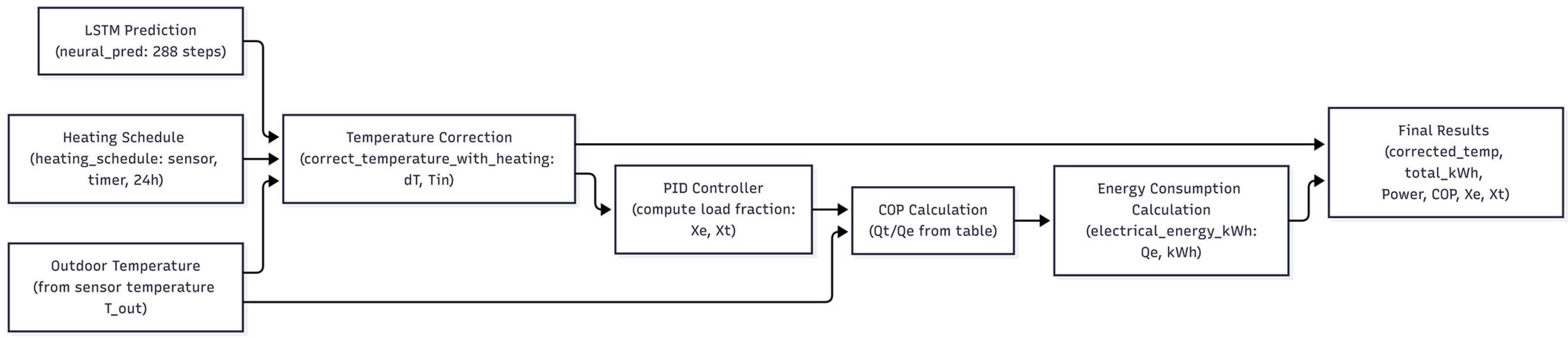
Following
Figure 2, the coefficient of performance (COP) is modelled by interpolating the manufacturer’s data as a function of outdoor temperature and electrical load fraction. An additional correction factor of 0.95 is applied for outdoor temperatures below 15 °C to account for installation and transient effects. This results in real COP values that are typically 85–95% of the tabulated ones, which is consistent with extensive in situ measurements and systematic reviews of air-source heat pumps in real residential conditions [
18,
19].
Based on the calculated COP, the thermal output and electrical power input are determined dynamically, with nominal and minimum capacities adapted to the prevailing external conditions. The model also tracks the dimensionless electrical (Xe) and thermal (Xt) load fractions to analyse deviations from nominal efficiency. The simulation framework supports various operating modes, including temperature-controlled operation (e.g., switch-on threshold of 19.5 °C), time-controlled on/off cycles, and continuous 24-h operation.
In the hybrid approach, the physical model is coupled with an LSTM-based predictive model, and their outputs are combined through adaptive weighting. This enables a realistic simulation of indoor temperature dynamics and electricity consumption under varying climatic and operating conditions.
The performance characteristics of the Toshiba SEIYA RAS-18J2KVG R32,Toshiba Corporation, Tokyo, Japan [
15] air-to-air inverter heat pump used in the simulations are given in
Table 2. The table presents heating capacity and electrical power input as a function of outdoor temperature and electrical load fraction (
Xe). These data were obtained from the manufacturer’s COP tables and are used for dynamic interpolation within the physical model.
2.4. Data Splitting and Model Training Procedure
The dataset of 52,128 records was split chronologically into training (70%), validation (15%), and testing (15%) sets. The LSTM model was trained on the training set, while hyperparameters were optimised via 5-fold cross-validation on the validation set by selecting the configuration with the lowest validation loss. All closed-loop simulations presented in this paper were performed using the fixed trained model without any further retraining.
3. Creating a Hybrid Model
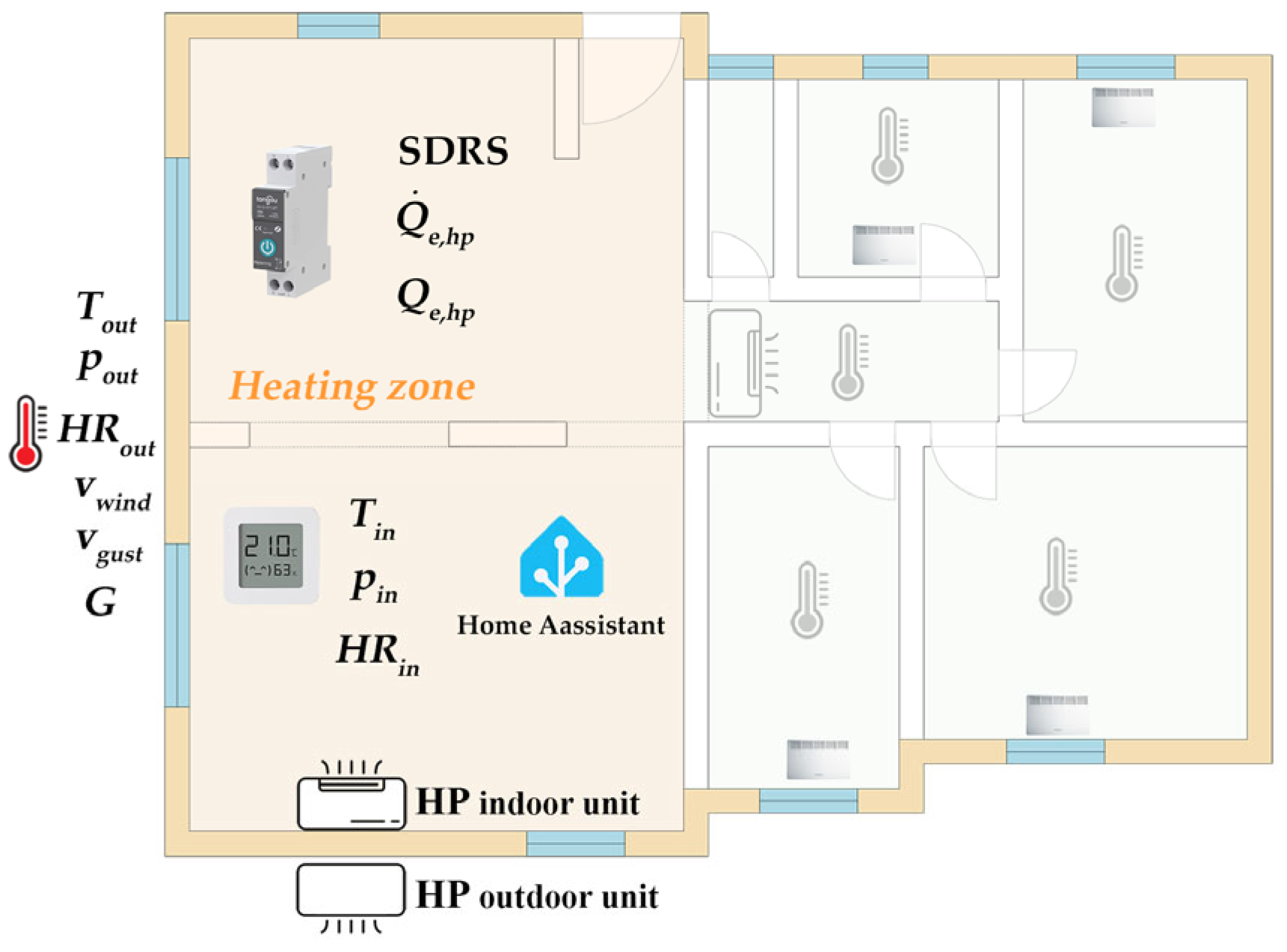
The hybrid model was developed based on the actual house shown in
Figure 3. It is an open-space residential building located in Zadar–Privlaka (southern Croatia, Dalmatia). Space heating is achieved by means of air-to-air heat pumps. The house is divided into two thermal zones, with each zone being served by a separate heat pump. In this paper, the focus is on modeling one zone of 57.2 m
2 [
15].
For the purposes of the physical model, the total heat transfer coefficient Utot was calculated based on the construction characteristics (thickness and thermal conductivity of the material, surface area of the elements), while the time constant τ was estimated from the ratio of heat capacity and losses. These values were used as starting points in the optimization process, whereby the final parameters Utot and τ were fine-tuned to the measured data from the real system, thus ensuring high physical accuracy of the model.
The indoor unit of the Toshiba SEIYA RAS-18J2KVG, Toshiba Corporation, Tokyo, Japanheat pump is wall-mounted at a height of 2.7 m in the living room, as shown in the simplified 2D schematic in
Figure 3. Air is drawn in from the top of the unit and blown downward into the room. The outdoor unit SEIYA RAS-18J2AVG is installed directly on the opposite side of the external wall, resulting in the minimum allowable refrigerant pipe length. All pipes are thermally insulated to minimise heat losses and ensure optimal operation. Room temperature is measured by three independent sensors positioned at a height of 1.5 m. The built-in sensor of the indoor unit (located at approximately 2.6 m) registers higher temperatures due to thermal stratification and is therefore not used for control purposes. The 1.5 m sensors provide more representative values for the occupied zone and are used for automation and comfort control.
3.1. Data Collection
The data used to calibrate the physical model and develop the hybrid model were collected through the home automation system during the 2024/2025 heating season in a residential building on the Croatian Mediterranean coast [
15]. The analysed period covers the winter season (November–April), providing representative thermal dynamics under dominant heating conditions. In total, 52,128 time-stamped records were collected and used for physical model calibration, LSTM training, and hybrid model validation. Indoor temperature was measured simultaneously with three co-located low-cost sensors (Aqara and Xiaomi Air Gradient) that exhibited excellent mutual agreement, with differences well within their specified accuracy of ±0.5 °C. The achieved model calibration RMSE (≈0.076 °C) is substantially lower than this sensor uncertainty, confirming the reliability of the validation results.
3.2. Measured Variables
The dataset was collected through the IoT platform developed in the previous paper [
15] and includes internal and external climate variables, energy parameters of the system, and meteorological influences. The measured quantities include indoor and outdoor air temperature, relative humidity, atmospheric pressure, electrical power and operating condition of the inverter heat pump (5 kW), wind speed and gusts, and global solar radiation. In addition, cyclical time features (hour of the day and day of the year) were used. The data was collected with a resolution of 5 min. All variables and their application in the model are shown in
Table 3.
3.3. Data Processing and Selection
Raw data is pre-filtered to remove invalid and missing tracks and timed to a unique 5-min raster. For the calibration of the physical model, night segments without active heating were selected, thereby minimizing the impact of solar gains and system control actions. Additional criteria include a minimum segment duration of 2 h and a sufficient change in the internal temperature, to ensure reliable identification of the parameters.
For the proposed model, complete time series, including exogenous meteorological variables, were used, with standardized data normalization.
3.4. Application in Models
The collected and processed data were used to calibrate key parameters of the physical model (e.g., Utot and τ) and to train and validate the LSTM component of the hybrid system. This ensured the empirical validity of the simulations and the robustness of the model in changing winter conditions.
3.5. Calibration of Physical Model Parameters
The calibration of the parameters of the total heat loss coefficient
Utot (W/K) and the time constant
τ (s) was carried out on the basis of data collected by the home automation system (Home Assistant, open-source platform developed by Nabu Casa, USA) during the heating season of 2024/2025 [
15] on the test residential building. The data includes indoor and outdoor temperature, humidity, electrical power, heat pump status, solar radiation and wind speed, with a focus on nighttime periods without active heating to isolate the natural cooling dynamics and minimize the impact of external disturbances.
These values serve as initial conditions for numerical optimization, ensuring physical reality and stable convergence. Optimization of the parameters total loss coefficient (W/K) and time constant τ (s) was performed by nonlinear least squares regression, using the Levenberg–Marquardt algorithm to minimize the square error between the measured and modeled internal temperature. Night periods were chosen due to stable boundary conditions and minimal impact of solar gains, thus increasing the accuracy of identification.
For these periods, the dynamics of the system is described by a simplified differential equation from the general physical model (see 2.2), excluding heating (
=
0) and solar gains
. The dynamics of the system are described by the differential equation without heating:
with an analytical solution in exponential form:
where the parameters
are optimized by minimizing the target function:
Parameter constraints () are set to ensure physically realistic values and stable convergence. The model does not include multi-zone dynamics or explicit solar gains, which is acceptable for night segments.
The implementation includes numerical integration of RK4 for model validation. The segments were selected according to the following criteria: periods without heating (heat_on = 0, power < 220 W), duration ≥ 2 h and temperature change ≥ 0.5 °C, which ensures sufficient dynamic variation for a reliable fit. The resulting optimized parameters of the physical model are presented in
Table 4.
Optimized values were obtained for RMSE = 0.076 °C and R2 = 0.94, which shows a very good agreement between the model and the measurements. This calibration ensures high reliability of the physical model in real-world conditions, supporting integration into a hybrid system for energy efficiency simulations.
3.6. A Python-Based Hybrid Modelling Framework
The hybrid model was developed in the Python (ver. 3.13.5) programming language as a platform-independent solution that can run on Windows, Linux and Raspberry Pi systems. This model combines a physical and data approach: an LSTM-type neural network was trained in a Keras (ver. 3.13)/TensorFlow (ver. 2.20) [
20,
21] environment to predict indoor temperature based on historical measurements (temperature, humidity, heat pump operation), while the physical part of the model was implemented using the NumPy (ver. 2.3.2) [
22,
23] and SciPy (ver. 1.16.1) [
24,
25] libraries through numerical simulation of the energy balance of the space using the fourth-order Runge–Kutta method.
Input data is loaded from CSV files or directly from the home automation system (Home assistant) and normalized using the MinMaxScaler algorithm [
26], and model training includes mechanisms such as EarlyStopping and ReduceLROnPlateau to prevent overlearning. Hybrid integration is achieved by adaptive weighting between the physical and neural models, while the control of heat pump operation is based on a proportional–integral–derivative (PID) controller.
The script enables simulation of system operation in time horizons from a few days to multi-day scenarios, with the calculation of performance metrics such as RMSE, MAE, MAPA and NMB and energy efficiency indicators. The results are visualized graphically to analyze the stability and behavior of the model under real climatic conditions. The actual coefficient of performance (COP) of the heat pump is calculated per energy consumed based on actual measurements of electrical power and temperatures, using the interpolation of the manufacturer’s data with the iterative determination of load fractions (Xe and Xt) for real installation conditions. The calculation was performed in a Python script using the RegularGridInterpolator, with a check of consistency with the electricity meter.
The neural model can be exported to the ONNX (Open Neural Network Exchange) format [
27], which ensures interoperability and performance in different software environments and on devices with limited resources. Such an approach allows the model to be implemented on “edge” platforms and its integration into real energy management and home automation systems.
3.7. Training and Generalization Performance of the LSTM Model
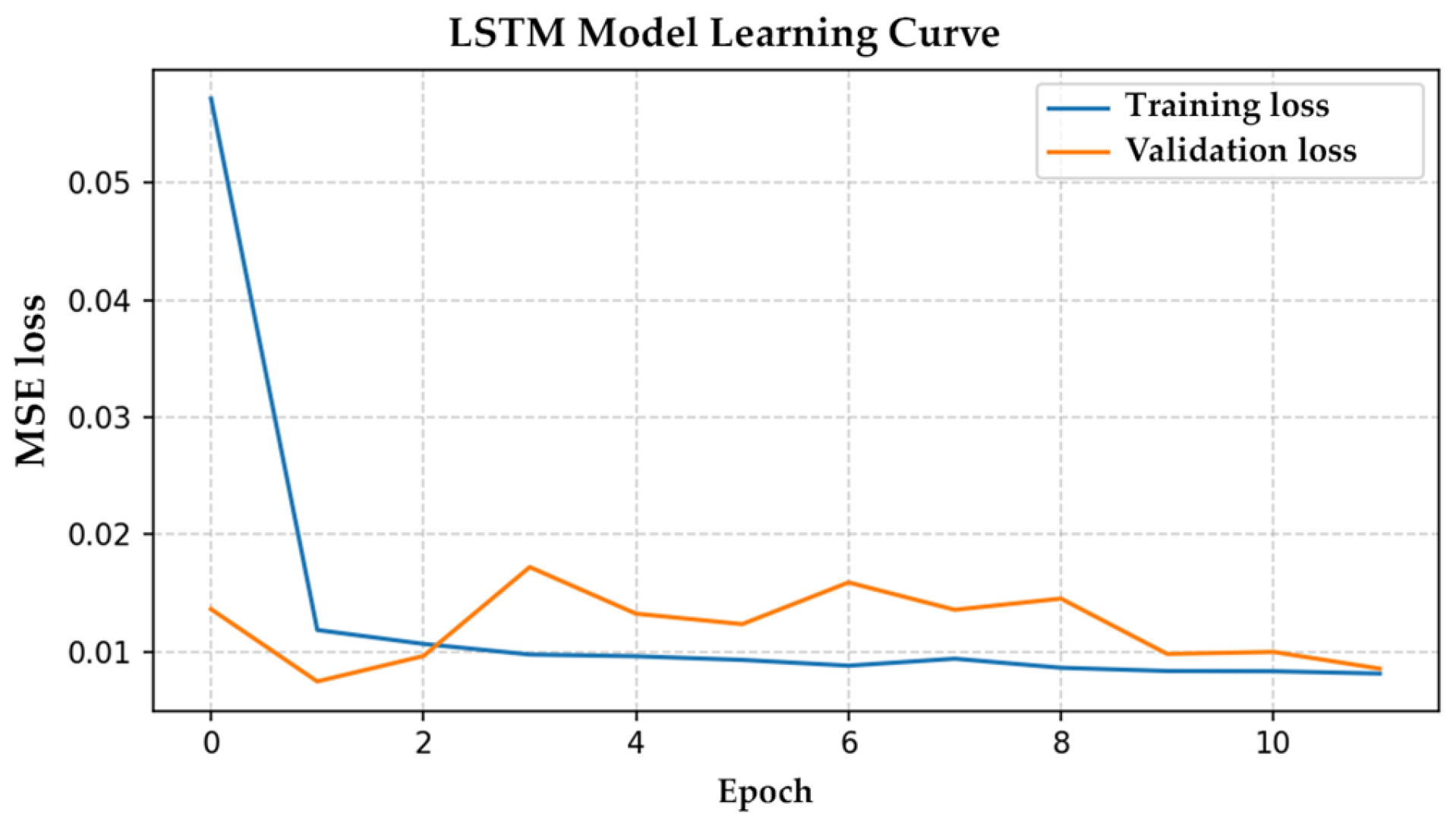
The LSTM model was trained using early stopping and adaptive learning rate reduction (ReduceLROnPlateau) in order to achieve stable convergence and prevent overfitting. The learning curve presented in
Figure 4 shows a rapid decrease in both training and validation loss during the initial training phase, followed by a stable convergence with only minor oscillations in the validation loss.
The small gap between the training and validation losses throughout the training process indicates that the model generalizes well and does not exhibit significant overfitting. The early stabilization of the loss values suggests that the input variables provide sufficient information for capturing the short-term thermal dynamics of the building zone.
On the independent test dataset, the model achieves MSE = 0.0131, corresponding to RMSE ≈ 0.11 °C, which represents a high level of predictive accuracy in the context of building thermal dynamics. The difference between the validation and test performance remains small, further confirming the stability and generalization capability of the trained model.
The obtained results indicate that the LSTM component successfully captures short-term system dynamics and local nonlinear effects that are not explicitly represented in the physical model. At the same time, the relatively small prediction error suggests that the data-driven component does not dominate the prediction process but rather acts as a corrective layer over the physics-based formulation.
Such a distribution of roles confirms the suitability of the hybrid modeling approach, where the physical model ensures energy consistency and long-term stability, while the LSTM component improves short-term prediction accuracy and adapts the model to changing operating conditions.
These findings support the interpretation of the proposed hybrid framework as a physics-informed modeling approach, in which the data-driven component compensates for unmodeled influences such as user behavior, air infiltration, or microclimatic variations, without disrupting the underlying physical structure of the model.
4. Simulation Scenario and Model Validation
An extensive numerical simulation of a hybrid model for predicting the operation of an inverter heat pump with a nominal output of 5 kW was carried out in this paper. Three main scenarios were evaluated: rolling one-day simulations (day-to-day with realistic initial conditions), continuous 3-day simulations and one 15-day continuous simulation. The simulations covered a period of 20 days, starting on 4 February 2025, in a typical winter season.
4.1. Simulation Settings
The simulations were carried out with a time step of 5 min, which corresponds to the resolution of the measurement data. The target indoor temperature is set at 21 °C. The operation of the heat pump is regulated by a proportional–integral–derivative (PID) controller with a dead zone (deadband 0.03–0.1 °C), an anti-windup mechanism and a minimum load fraction to prevent oscillations and frequent cycling.
The hybrid model uses an adaptive weighted coupling of LSTM prediction and physical model results according to Equation (4). Meteorological inputs (outside temperature, wind speed and solar radiation) are taken from actual measurements. The room temperature is limited to a physically realistic range (5–35 °C).
4.2. Objectives and Criteria of Validation
The main objectives of the simulation were:
Assessment of the energy efficiency of the system (total electricity consumption and COP);
Analysis of the dynamic response of the indoor temperature during active heating and periods without heating;
Evaluation of the stability and limitations of the hybrid model compared to the pure physical model under changing meteorological conditions.
Validation was carried out by comparing simulated and measured temperature profiles and energy quantities using standard metrics (RMSE, MAPE, NMB and R2). Special attention is paid to the behavior of the models on different time horizons. Several-day off-period breaks of the heating system were used as a sensitive test of the correctness of calibrated parameters ( and τ).
The quantitative analysis also included the energy consistency of the models, while the results were stored in the form of time series and graphical representations (temperature profiles, thermal output, electrical power and COP). These representations serve as a basis for comparing the performance of the hybrid and physical models and for identifying their limitations in the real conditions of the Mediterranean climate.
4.3. Simulations
4.3.1. One-Day Simulation
A one-day simulation (scenario S1) was conducted as an initial validation scenario with the aim of assessing the dynamic response of the model and the influence of the hybrid weighting ω on the prediction of internal temperature and energy indicators of the system. The simulated results were compared with the measured data of the actual operation of the heat pump and the associated space, where scenario S0 represents a set of data based on the measured values of the actual operation of the heat pump, and scenario S1 represents the simulation results obtained for different values of the weight factor.
This short-term scenario allows us to assess the stability of the control, the response of the model to changes in external conditions, and the sensitivity of the simulation to the weighting between the physical and data-driven parts of the model before conducting multi-day simulations. Special emphasis is placed on the reproduction of the internal temperature of the Tin space, electricity consumption Qe, and the estimation of the derived energy quantities of the coefficient of efficiency (COP) and system load (Xe, Xt).
Table 5 shows a summary of the characteristic variables for the corresponding weighting factor values. The results show that the change in the ω factor has a very limited impact on the average indoor temperature, while differences appear in the estimated energy indicators, especially in energy consumption and derived COP values. This confirms that the one-day simulation is primarily used to assess the dynamic response of the model and the initial analysis of the impact of hybridization, while the full evaluation of the stability and long-term behavior of the model is carried out in multi-day scenarios.
Although the one-day simulation shows an increase in the estimated COP of the hybrid model, this effect does not represent a real improvement in energy efficiency, but is a consequence of short-term load redistribution, which proves to be unstable in continuous simulations. In this sense, the contribution of the data-driven component in the short term remains limited and is manifested primarily through a change in load distribution, and not through an improvement in temperature accuracy.
4.3.2. Multi-Day Simulation
Scenario S2
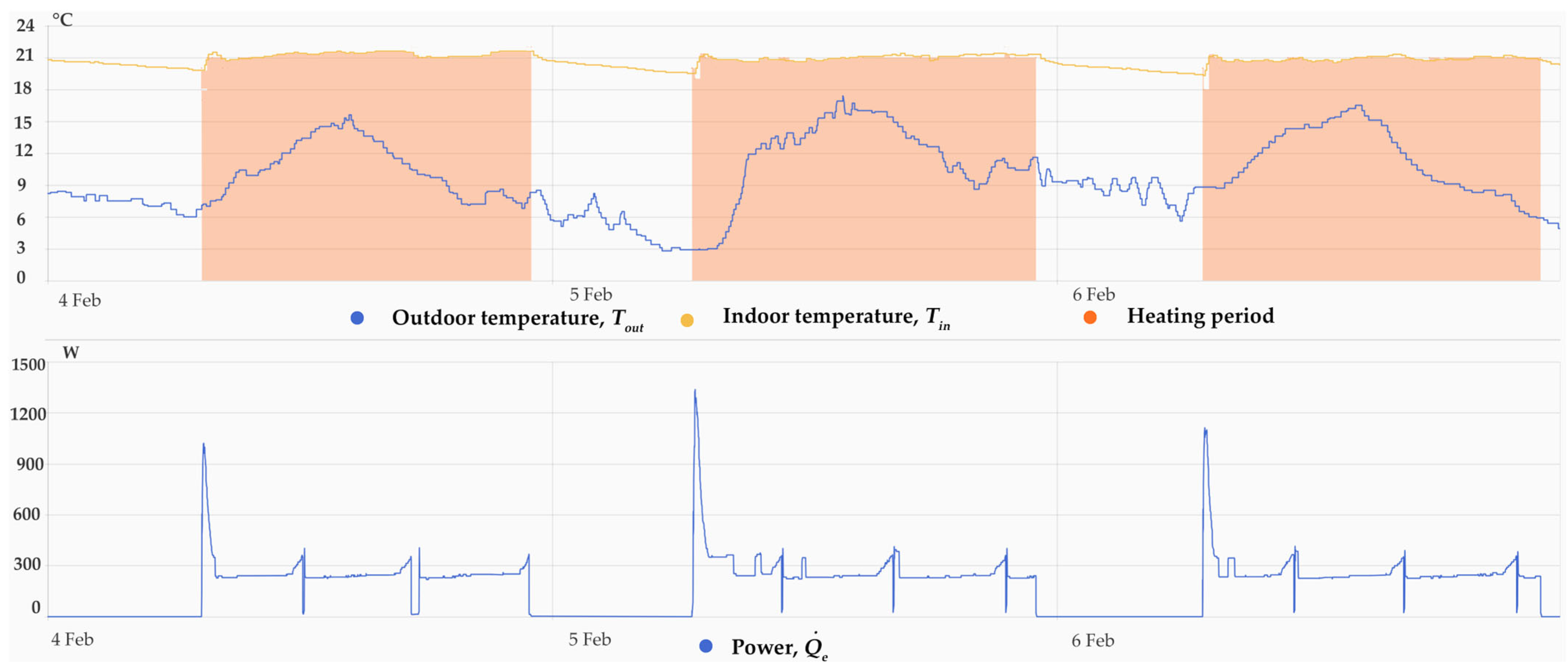
Multi-day simulations include characteristic periods of 3 days (scenario S2,
Figure 5) and an extended cycle of 20 days, which includes 15 days of continuous operation (scenario S3,
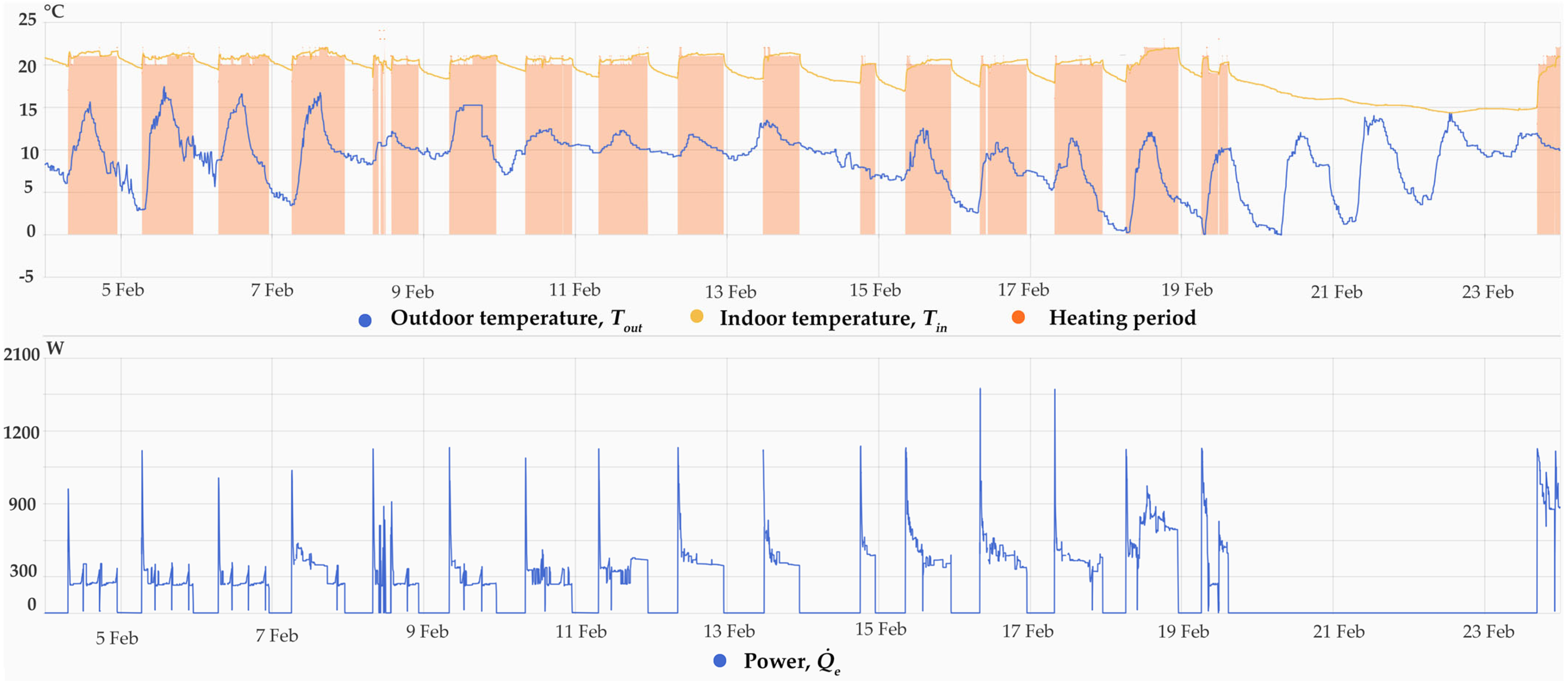
Figure 6) and a three-day heating interruption (scenario S4, e.g., from 20 to 23 February 2025). The energy quantities for the 3-day continuous simulation (scenario S2) are summarized in
Table 6, while the energy quantities and performance metrics for the 15-day continuous simulation (scenario S3) are summarized in
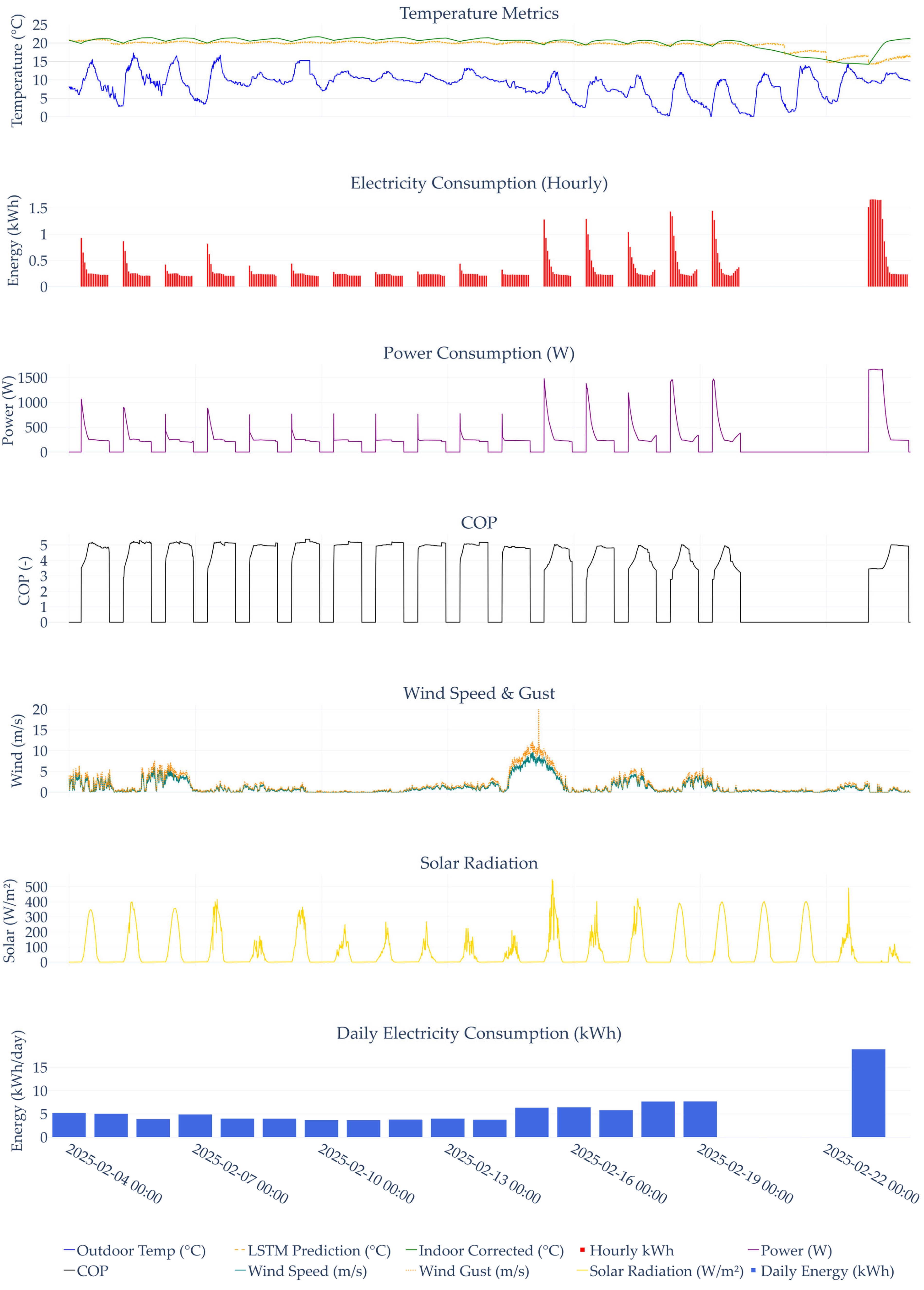
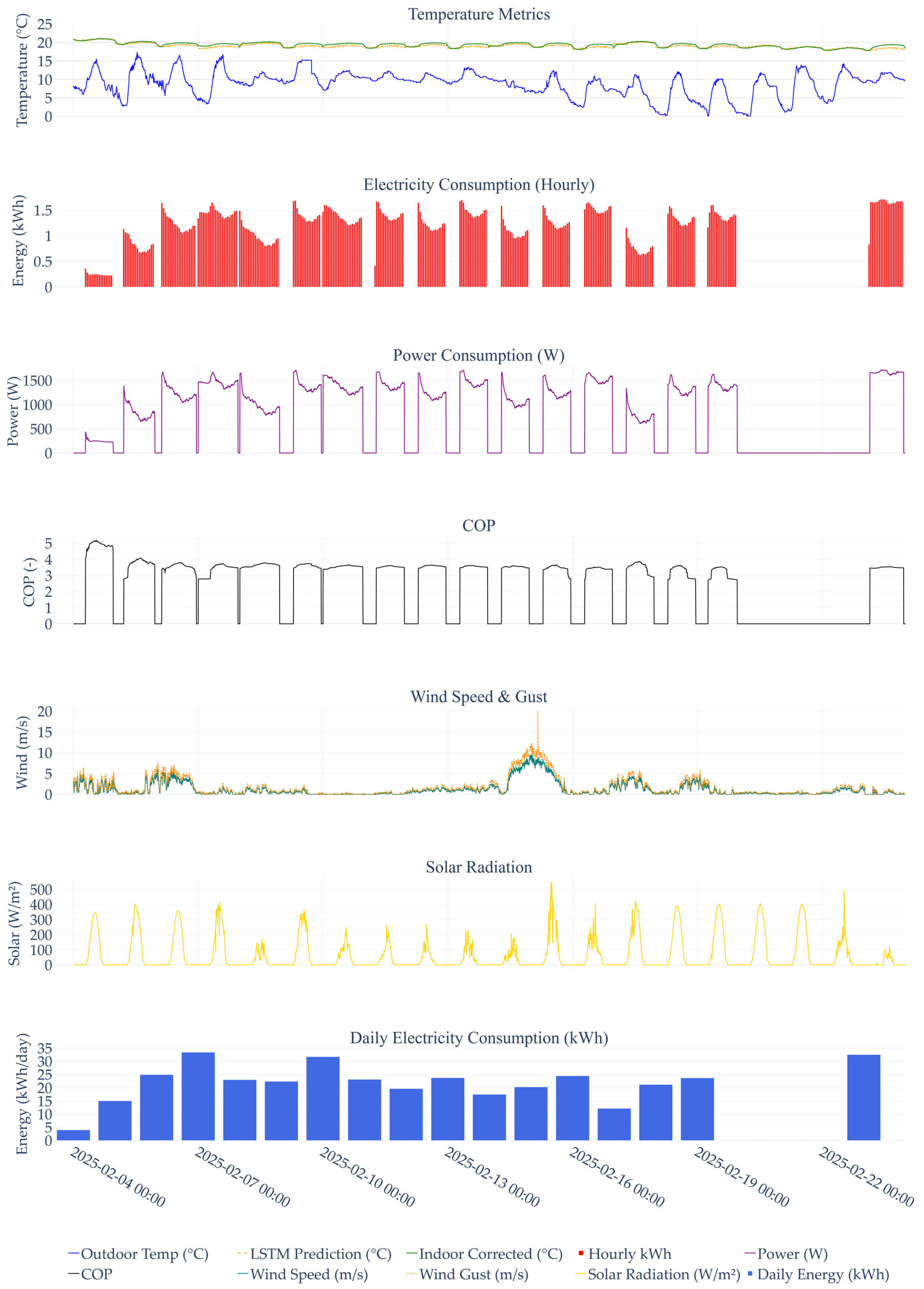
Table 7. The temporal evolution of key variables (indoor temperature, electrical power, and coefficient of performance) during the 20-day simulation period is shown in
Figure 7 (pure physical model, ω = 0.0) and
Figure 8 (hybrid model, ω = 0.1).This approach allows for an in-depth assessment of the integration of LSTM predictions, based on 24-h history and short-term forecasts, with a physical model, with an emphasis on the impact of meteorological fluctuations and weather parameters on the overall stability of the hybrid system.
A special focus is placed on the period without active heating, where the natural cooling of the building is analyzed, key parameters such as total heat loss () and time constant (τ) are validated, and the response to system restarts is examined.
These findings serve as the basis for future optimizations, including adaptive weight factor adjustment, analysis of the influence of constants, and scaling capabilities on objects with different thermal properties.
Figure 5.
Measured value of heat pump operation, Home Assistant history, 3 days.
Figure 5.
Measured value of heat pump operation, Home Assistant history, 3 days.
Table 6.
Summary of energy quantities for the 3-day continuous simulation (4–6 February 2025, Scenario S2).
Table 6.
Summary of energy quantities for the 3-day continuous simulation (4–6 February 2025, Scenario S2).
| Parameter | Mark | Units | Scenario S0 * | Scenario
S2 | Note |
|---|
| Weight factor | ω | — | — | 0.0 | 0.05 | 0.1 | — |
| Average internal temperature | Tin | °C | 20.83 | 20.89 | 20.26 | 20.16 | Temperature drop in hybrids |
| Electricity consumption | Qe | kWh | 12.80 | 14.18 | 39.61 | 47.52 | A jump in consumption in hybrids ω > 0, the beginning of divergence |
| Coefficient of Performance | COP | — | 4.47 | 4.64 | 3.78 | 3.69 | Decline in COP in hybrids—a sign of degradation |
| Average electrical load | Xe | % | 29.9 | 17.4 | 40.0 | 46.4 | Increase in load in hybrids |
| Average heat load | Xt | % | 35.2 | 23.1 | 44.2 | 50.0 | Increase in load in hybrids |
Scenario S3
Figure 6.
Measured value of heat pump operation, Home Assistant history, 20 days.
Figure 6.
Measured value of heat pump operation, Home Assistant history, 20 days.
Table 7.
Summary of energy quantities for a 15-day continuous simulation (4–18 February 2025, Scenario S3).
Table 7.
Summary of energy quantities for a 15-day continuous simulation (4–18 February 2025, Scenario S3).
| Parameter | Mark | Units | Scenario S0 * | Scenario
S3 | Note |
|---|
| Weight factor | ω | — | — | 0.0 | 0.05 | 0.1 | — |
| Average internal temperature | Tin | °C | 20.10 | 20.83 | 19.52 | 19.58 | Systematic temperature drop in hybrids |
| Electricity consumption | Qe | kWh | 87.00 | 72.31 | 315.55 | 316.42 | Extreme jump in consumption in hybrids—full divergence |
| Coefficient of Performance | COP | — | 3.97 | 4.44 | 3.48 | 3.51 | Decline in COP in hybrids |
| Average electrical load | Xe | % | 40.6 | 18.2 | 72.4 | 71.5 | Increase in load in hybrids at ω = 0.05 |
| Average heat load | Xt | % | 45.2 | 23.8 | 74.3 | 73.4 | Load increase in hybrid ω = 0.05 |
Scenario S4—Off Period
Model validation was conducted using a 72-h dataset collected during a heat pump off-period, enabling assessment of the building thermal envelope model under passive cooling conditions. The simulated indoor temperature showed strong agreement with measurements, with a Pearson correlation coefficient of r = 0.976, indicating that the model reliably reproduces the temporal dynamics of indoor temperature decay. Error metrics confirm good predictive performance for a simplified single-zone thermal model. The mean absolute error was (MAE) 0.83 °C, while the root mean square error (RMSE) reached 1.00 °C. These values fall within the range typically reported for building thermal simulations under real operating conditions, where uncertainties related to infiltration, internal gains, and thermal mass distribution are unavoidable. The simulation successfully captured the overall cooling trend and thermal inertia of the building envelope during passive operation. Remaining discrepancies are attributed primarily to unmodeled internal heat gains, variability in air exchange rates, and spatial thermal heterogeneity not represented in the lumped parameter model. Despite these limitations, the strong correlation and moderate error levels indicate that the calibrated model provides a reliable representation of dominant heat loss mechanisms during off-cycle periods. These results support the suitability of the model for further use in system-level simulations and control strategy evaluation, where accurate representation of envelope dynamics during heat pump cycling is essential.
Figure 7.
Multi-day (20 days) simulated values of a hybrid heat pump model, ω = 0.0.
Figure 7.
Multi-day (20 days) simulated values of a hybrid heat pump model, ω = 0.0.
Figure 8.
Multi-day (20 days) simulated values of a hybrid heat pump model, ω = 0.1.
Figure 8.
Multi-day (20 days) simulated values of a hybrid heat pump model, ω = 0.1.
5. Simulation Results and Discussion
The assumptions and calibration of the first-order physical model (energy balance, wind correction, and solar gains) are directly reflected in all simulation results. Any deviation observed in the hybrid model can therefore be attributed to the LSTM correction rather than to deficiencies in the physical component.
A comparison of the simulated temperature profiles with the measured data confirms that both models capture the basic thermal dynamics during active heating and off-periods (off-period validation: r = 0.976, RMSE = 1.00 °C). However, the performance of the hybrid model depends significantly on the simulation horizon and the implementation method (rolling versus continuous).
5.1. Comparison of Simulated and Measured Temperature Profiles
On short- and medium-term horizons (1–3 days), the pure physical model achieves lower RMSE values for indoor temperature. In a 15-day continuous simulation, the physical model better maintains the target temperature (average 20.83 °C, close to the setpoint of 21.0 °C), while the hybrid model causes a significant drop in the average indoor temperature (19.52 °C at ω = 0.05 and 19.58 °C at ω = 0.10). Although the hybrid model shows a slightly lower RMSE_T_corr on this horizon (0.76–0.78 °C vs. 0.94 °C), this result does not indicate better performance. A lower RMSE is an artifact of a systematic underestimation of temperature: the hybrid model consistently predicts a lower mean, thereby reducing variation around the wrong mean temperature. The physical model, in contrast, better maintains the target temperature but shows a higher RMSE due to larger deviations around the higher average. Therefore, RMSE is not a reliable indicator of model quality here.
The energy quantities and performance metrics for the 15-day continuous simulation (scenario S3) are summarized in
Table 7. The performance metrics for the different simulation horizons and hybrid weights (including 1-day and 3-day periods) are given in
Table 8. The “Rolling 15 days (day-for-day)” scenario represents the average of metrics from 15 separate one-day simulations, where each day is simulated independently with the real measured initial conditions of that day. The “Continuous 3 days” and “Continuous 15 days” scenarios were implemented as full continuous simulations without resetting the state of the LSTM model between days. All metrics are calculated in relation to the actual measured data (scenario S0). The degradation slope (°C/day) represents the linear increase in the absolute error of the internal temperature prediction over time, calculated by linear regression of the daily absolute deviations of the simulated and measured temperature.
5.2. Analysis of Energy Indicators and Impact of Hybrid Weighting
The analysis of energy indicators shows that the hybrid model causes a systematic decrease in the average indoor temperature in continuous simulations (19.52 °C at ω = 0.05 and 19.58 °C at ω = 0.10). This negative bias causes the PID controller to continuously increase the load on the heat pump in an attempt to compensate for the temperature. The consequence is drastically higher simulated electricity consumption (315–316 kWh) compared to the physical model (72 kWh) and real measurements (~87 kWh).
The extremely high MAPE_Qe (311–321%) is precisely the result of this compensatory overpower in the simulation. The relative error becomes extremely large because too high a simulated consumption is compared with an actual lower consumption at a higher indoor temperature.
At the same time, there is a change in the sign of NMB_Xe: in the rolling approach, the hybrid model shows negative bias (–60.64% to –61.88%), while in the continuous simulation it becomes positive (+35.17% to +77.63%). This change reflects the different behavior of the model—in rolling mode, LSTM tends to underestimate the need for heating, while in continuous mode, the accumulated temperature error leads to a compensatory increase in the load factor (higher Xe).
These results confirm that the apparent improvements in short-term simulations are not due to better prediction, but to the implicit virtual heat flux of the LSTM correction, which is analyzed in more detail in
Section 6.
5.3. Model Behavior During System Outages
In multi-day simulations with heating breaks, the model faithfully reproduces the exponential temperature drop (RMSE ≈ 1.00 °C during the off-period), thus confirming a good calibration of heat loss parameters and time constants. A similar level of accuracy in these conditions is shown by a pure physical model.
5.4. Role of the Physical Model, Hybridisation Limits and Influence of the Time Horizon
The calibrated physical model achieved high accuracy in periods without heating (RMSE ≈ 1.00 °C), confirming that the energy-balance approach reliably describes the dominant dynamics when the parameters (Utot, τ, internal gains) are correctly estimated. Under such conditions, the contribution of LSTM is limited, as the physical model already captures most of the variability. Hybridization does not bring significant improvement, and can cause degradation due to sensitivity to distribution shift outside the training domain.
The analysis of simulations shows a pronounced dependence of performance on the time horizon (
Table 8). For short-term rolling simulations (up to 24 h), the hybrid model provides marginal adaptive correction, slightly improving energy prediction (MAPE_Qe ≈ 34%) at the cost of reduced temperature accuracy (RMSE ≈ 0.8 °C vs. 0.3 °C for the physical model). However, in longer continuous simulations (15 days), a systematic degradation emerges: the hybrid models exhibit a significant negative bias (−0.5 to −0.6 °C), causing the average indoor temperature to drop to approximately 19.5 °C—well below the setpoint (21 °C) and below the physical model (20.83 °C). At the same time, energy inconsistency becomes extreme, with MAPE_Qe exceeding 300% (compared to 27% for the physical model). The lower RMSE of the hybrid models (0.76–0.78 °C vs. 0.94 °C) is therefore misleading—it reflects reduced variability around an incorrect mean, not improved physical fidelity. This, combined with the energy inconsistency from Chapter 5 (implicit virtual heat flow), confirms that apparent improvements (e.g., higher COP with lower consumption) are not realistic, but an artifact of the model. Hybrid models are not universally superior—their effectiveness depends critically on the quality of the physical calibration, the prediction horizon, and the preservation of energy conservation principles.
5.5. Specificities of the System and Climate Context
In the conditions of the Mediterranean climate, characterized by low heat loads and the complete absence of defrost cycles, the key challenge is the cyclic operation of the heat pump stabilized by PID regulation, with the average COP ranging between 3.5 and 4.9 (depending on ω). These results are consistent with extensive in situ measurements and systematic reviews of air source heat pumps in real-world residential settings (Chesser et al., 2021; Carroll et al., 2020) [
18,
19], which report similar COP values (most commonly 2.8–4.5) in temperate climates, with an emphasis on the high dependence on actual load, installation and climatic conditions.
5.6. Implications for Digital Twins and MPC
The results support the development of digital twins: physical models ensure interpretability and efficiency on edge devices, while hybrid models can compensate for uncertainties (e.g., weather forecasts). For MPC, a hybrid framework is relevant in short-term management, but requires consistency validation to avoid degradation.
5.7. Limitations of Research and Future Work
The present study is limited to a single residential building and one heating season in the Mediterranean climate, with the LSTM model trained on data lacking seasonal variation or changes in occupant behaviour.
Future work should include validation across different climatic conditions, multi-season training to improve generalisation, testing on other buildings and HVAC systems, and the integration of online learning or physics-informed neural networks. In addition, real-world model predictive control (MPC) scenarios with simultaneous optimisation of energy consumption and thermal comfort should be explored.
Comparison of the proposed hybrid model with alternative machine learning approaches (e.g., Random Forest, XGBoost, or standalone LSTM) was outside the scope of the present study, which focused specifically on the interaction between a well-calibrated physical model and LSTM-based correction in closed-loop operation. Such comparisons are planned for future work.
6. Energy Inconsistency of the Hybrid Physical-Data Model
Hybrid models that combine physical equations with data-driven components offer the possibility of compensating for phenomena that are difficult to describe with purely physical approaches. However, when the data-driven component directly corrects the system state without an explicit adjustment to the energy balance, a fundamental problem of energy inconsistency arises. This paper demonstrates that such inconsistency can produce apparently improved results that are not physically grounded, particularly in long-term simulations.
6.1. Introduction to Hybrid Modeling
When a data-driven component (here, LSTM) directly corrects the system state—the indoor temperature—without a corresponding term in the energy balance equation, a fundamental inconsistency arises. The LSTM correction effectively acts as an implicit virtual heat flux: it adds or removes thermal energy from the space without causing any change in the actual heat pump output, internal gains, or transmission losses. This chapter formalizes this concept mathematically, quantifies it using simulation results, and illustrates how it distorts controller behaviors and long-term energy predictions. The analysis shows that short-term apparent improvements are not physically meaningful and that energy consistency must be explicitly enforced for reliable hybrid modelling in real-world applications.
6.2. Description of the Hybrid Approach and Correction
In the proposed model, the indoor temperature is computed as a weighted combination of the physical model output and the LSTM prediction (Equation (4),
Section 2.3). While this formulation improves short-term temperature prediction accuracy, it simultaneously introduces an implicit virtual heat flux. The LSTM correction modifies the estimated temperature state, but this thermal effect is not compensated in the energy balance of the space nor in the calculation of heat pump output and electrical consumption.
6.3. Implicit Energy Balance of the Hybrid Model
In a pure physical model, the change in internal energy of space is given by Equation (1) from the methodology, since internal energy is proportional to temperature (
U = Ceq⋅T); this equation can also be written in the form of a change in internal energy:
where
represents the net effect of all real energy flows: heat pump output, effective internal gains, and transmission losses through the building envelope.
In the hybrid model, the LSTM correction alters the temperature directly, which is equivalent to introducing an additional fictitious term:
where
is the implicit virtual heat flux induced by the LSTM correction:
This term does not correspond to any actual heat flux—it is a pure mathematical artefact.
6.4. Implications for Regulation, Energy Consumption and Physical Consistency
The LSTM temperature correction directly affects the PID controller’s setpoint error, but the direction of this effect is not consistent across simulation horizons. In short-term rolling simulations (1 day, ω = 0.05–0.10), the correction typically introduces a positive bias, resulting in higher simulated indoor temperature, reduced control error, and an artificially lower energy consumption and higher COP — the so-called “free lunch” artefact. In continuous multi-day simulations (3 and 15 days), however, the same correction develops a negative bias (lower simulated temperature), increasing control error and leading to excessive simulated electricity consumption (up to 316 kWh vs. 72 kWh after 15 days, see
Table 7).
Both behaviours originate from the same fundamental issue: the hybrid model modifies the thermal state without accounting for the corresponding energy input or removal. This non-conservative perturbation violates the energy balance equation. The cumulative virtual heat flux introduced by the LSTM correction over the 15-day period was estimated at approximately +248 kWh (ω = 0.05) and +244 kWh (ω = 0.10). These values closely match the observed excess electricity consumption of 243–244 kWh relative to the pure physical model, confirming that the LSTM correction acts as a non-conservative perturbation outside the physical energy balance.
Physical consistency
In a real physical system, any sustained change in mean indoor temperature under identical boundary conditions must be accompanied by a corresponding change in net heat input. The hybrid model produces combinations that are physically impossible: higher temperature with lower consumption (short horizons), or dramatically higher consumption with lower temperature (long horizons).
This inconsistency is embedded at the formulation level: the state correction introduces or removes heat without a corresponding term in the energy balance equation.
This phenomenon can be understood through an analogy with numerical integrators in dynamics. The physical model preserves the fundamental structure of the system—every temperature change must pass through a real heat flux (). The LSTM correction, however, acts as a non-conservative perturbation: it changes the state directly, without passing through the energy balance. The result is integrator drift—a small systematic bias accumulates over time, analogous to classical integrators that do not preserve the geometric structure of the system. The observed behaviour (smaller local RMSE accompanied by global energy drift) is exactly the expected outcome of such structural inconsistency. Most previous hybrid studies avoid this problem because they validate models in open-loop mode, without a closed control loop with a regulator.
6.5. Significance of Results for Hybrid Modelling
This work highlights three key implications for hybrid modelling in building energy systems:
Statistical performance metrics (RMSE, COP) can be misleading when state corrections lack explicit energy accounting.
Energy consistency must be enforced explicitly: without compensation for the implicit virtual heat flux, hybrid models risk becoming physically inconsistent, especially in long-term and closed-loop applications.
These findings provide practical guidance for developing reliable digital twins of heat pump systems: machine learning should enhance, not circumvent, the underlying physics. A well-calibrated physical model remains more robust for long-term simulations and edge deployment. Hybrid approaches can be valuable only if they include an explicit energy compensation loop.
7. Conclusions
This study demonstrates that hybrid physical–LSTM models do not offer a systematic advantage over a well-calibrated physical model when applied to the closed-loop control of an air-to-air inverter heat pump in Mediterranean climate conditions. The key innovations of this work are the use of an adaptive weighting mechanism (ω) between the physical and LSTM components and the explicit identification and quantification of the implicit virtual heat flux introduced by the LSTM correction. These contributions reveal a previously under-reported limitation of hybrid models: while they can produce apparently better short-term RMSE, they violate thermodynamic consistency in long-term closed-loop operation.
The physical model, calibrated and validated against 52,128 real IoT measurements from a residential building in Zadar, Croatia, provides high accuracy and serves as a thermodynamically consistent reference. In rolling one-day simulations, the hybrid model slightly degrades temperature prediction accuracy compared to the pure physical model. In continuous multi-day simulations (up to 15 days), it yields marginally lower RMSE values. However, this apparent statistical improvement is accompanied by systematic underestimation of indoor temperature and substantially higher simulated energy consumption. The discrepancy arises from an implicit virtual heat flux introduced by the LSTM correction, which violates energy balance within the closed control loop and accumulates as integrator drift over time.
These results indicate that short-term statistical metrics such as RMSE are insufficient for evaluating hybrid models intended for real-world operation. Well-calibrated physical models exhibit greater long-term stability, interpretability, and energy consistency. Hybrid approaches may provide useful short-horizon corrections, but they require explicit mechanisms to preserve thermodynamic consistency before deployment in model predictive control (MPC) or digital twin applications.
In 15-day continuous simulations, the hybrid model (ω = 0.05–0.10) caused an indoor temperature underestimation of 1.25–1.31 °C and increased electricity consumption by more than 300% (316 kWh vs. 72 kWh) relative to the physical model. For practical applications on edge devices, the physical model remains the more reliable foundation.
Future research should focus on energy-consistent hybrid architectures, multi-season validation, and real-world MPC testing. Overall, this study confirms that hybrid modelling is not a universal solution, but a methodologically demanding approach that must remain firmly grounded in physical principles and rigorously verified for long-term thermodynamic consistency.