Successive Overrelaxation–Progressive Interpolation for Loop Subdivision Surfaces

Abstract

The Loop subdivision scheme is one of the most widely used approximation subdivision methods for generating smooth surfaces. However, the limiting surface of the Loop subdivision scheme does not interpolate the vertices of the original mesh and may exhibit shrinkage in certain cases. To overcome this limitation, we propose the Successive Overrelaxation–Progressive Iterative Approximation (SOR-PIA) method, which adjusts the positions of the original vertices so that the corresponding limit surface of the Loop subdivision scheme can interpolate the vertices of the given mesh. The optimal relaxation parameter for the SOR-PIA method is also provided. Compared to classical PIA, Weighted PIA (W-PIA), Hermitian and skew-Hermitian PIA (HSS-PIA), and Weighted Hermitian and skew-Hermitian PIA (WHSS-PIA), the proposed method converges faster while maintaining accuracy, as demonstrated by numerical examples.

1. Introduction

The reason why subdivision surface techniques are so common in computer graphics, animation, geometric modeling, and industrial design is that they are able to produce smooth surfaces of high quality based on relatively coarse control meshes. The subdivision schemes can be broadly categorized into two groups: interpolatory schemes and approximation schemes.

In interpolatory subdivision schemes, the limit surface interpolates the vertices of the original mesh. Some typical examples would be the Butterfly scheme [1], the improved Butterfly scheme [2], and the Kobbelt scheme [3]. Approximation subdivision schemes, on the other hand, generate smooth surfaces that are approximations, not interpolations of the original mesh vertices. 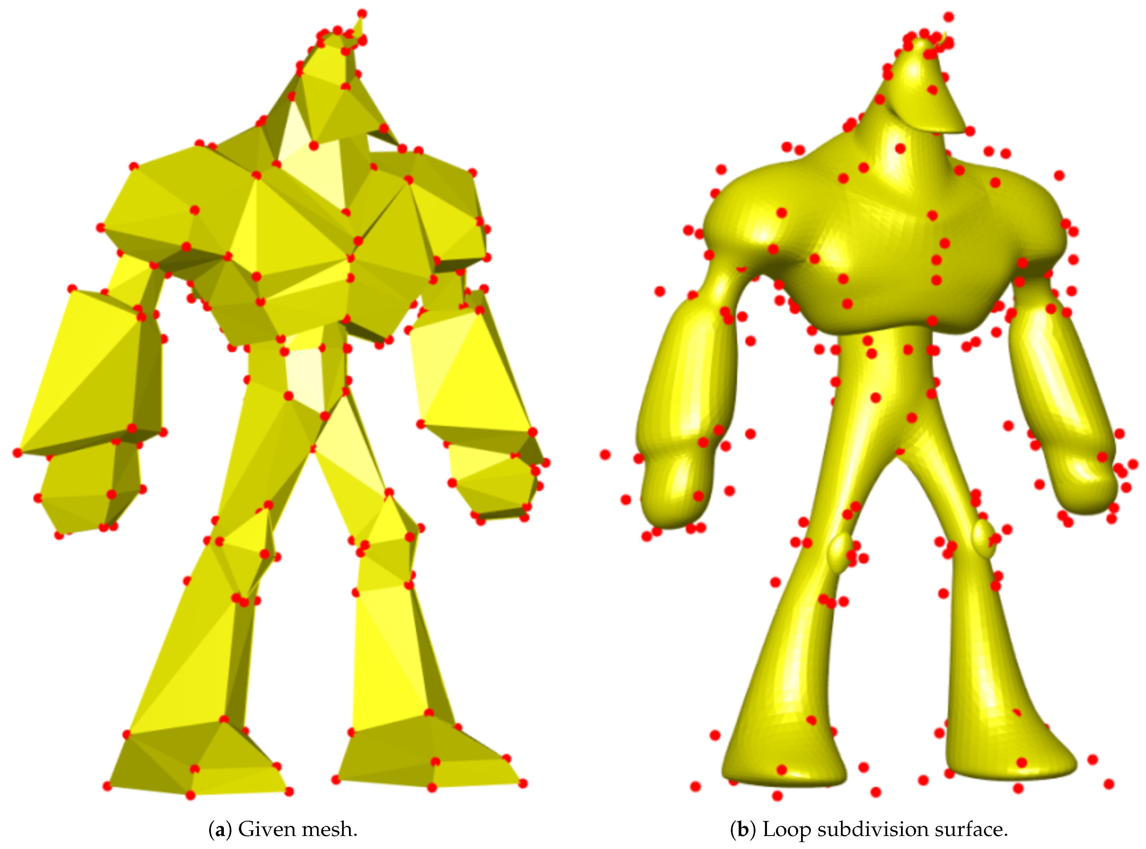Some classical examples of this class are the Loop subdivision scheme [4] and the Catmull–Clark subdivision scheme [5]. The main weakness of approximation schemes is that they can have a visible shrinkage of limit surfaces in some cases (see Figure 1).

Interpolatory schemes are subdivision schemes that can preserve vertex positions; however, irregular mesh topology is not always well-behaved and can give rise to objectionable artifacts in instances where the initial mesh has extraordinary vertices [1]. In triangular meshes, a vertex with a valence that deviates from the standard valence (for example, a valence other than six) is referred to as an extraordinary vertex. Such irregular vertices may lead to undesirable artifacts in interpolatory subdivision surfaces. In order to overcome this weakness, a number of researchers have suggested techniques that impose interpolation on approximation subdivision surfaces [6,7,8,9,10,11]. The first papers to use Progressive Iterative Approximation to Catmull–Clark and Loop subdivision surfaces were written by Chen et al. [6] and Cheng et al. [7], respectively. Such schemes are now called classical Progressive Iterative Approximation (PIA) of stationary subdivision schemes. Classical PIA is, however, known to have slow convergence.

Deng and Ma [8] proposed the Weighted PIA (W-PIA) to enhance convergence performance. An extension of acceleration techniques was to formulate Conjugate-Gradient PIA [9] and Gauss–Seidel PIA [10]. Recently, Hamza et al. [11] included Hermitian and skew-Hermitian splitting methods in the PIA framework and achieved faster convergence than classical PIA.

Recent studies have extended subdivision surface methodologies beyond conventional formulations, with particular attention given to enhanced smoothness regulation, adaptive refinement strategies, and application-oriented improvements. In particular, modified Loop and Catmull–Clark subdivision approaches have been introduced to improve surface fairness and minimize geometric artifacts, especially in the vicinity of extraordinary vertices [12,13]. Furthermore, optimization-based techniques have been employed to achieve a better balance between geometric fidelity and surface smoothness in subdivision modeling frameworks [14].

Liu et al. [15] introduced a neural subdivision framework that combines Loop subdivision topology with neural-network-based geometric refinement. In contrast to traditional subdivision schemes that depend on fixed linear masks, the proposed approach learns nonlinear subdivision rules directly from high-resolution mesh datasets using a self-supervised learning mechanism. The framework supports adaptive coarse-to-fine mesh generation, improves the preservation of geometric features, and alleviates common artifacts such as over-smoothing, volume shrinkage, and tessellation distortion associated with classical subdivision techniques.

More recently, subdivision surfaces have also been incorporated into isogeometric analysis [16]. These developments demonstrate that stationary subdivision schemes remain an active research area with increasing relevance in both theoretical and applied geometric modeling.

2. Problem Statement and Notation

Let $M=(V,E)$ represent an input triangular mesh, where $V={\left\{v_i\right\}}_{i=1}^m\subset {\mathbb{R}}^3$ is the set of control vertices and E is the edge set. Let $B\in {\mathbb{R}}^{m\times m}$ symbolize the Loop subdivision limit matrix, given that the limit positions of the control vertices are

$$V_{\infty }=BV,$$

(1)

where $V={[v_1,v_2,\dots ,v_m]}^T$ and $V_{\infty }$ assembles the corresponding Loop subdivision limit points.

The original mesh vertices are given by $V^{\left(0\right)}$. The subdivision surface interpolation problem considered in this paper is to determine a modified control mesh $V^{\ast }$, such that the Loop subdivision surface interpolates the original vertices, that is,

$$B{V}^{\ast }=V^{\left(0\right)}.$$

(2)

Throughout this paper, the superscript $\left(k\right)$ represents the iteration index, $\omega \in (0, 2)$ is the relaxation parameter used in the SOR iteration, and $\parallel ·\parallel$ denotes the Euclidean norm unless otherwise specified.

This paper is inspired by the effectiveness of classical iterative solvers of linear systems and suggests a new interpolation procedure as a progressive interpolation technique with the help of the successive overrelaxation (SOR) technique. The proposed SOR-PIA process will hasten the convergence of progressive interpolation of Loop subdivision surfaces, with interpolation accuracy being preserved. The interpolating surfaces result in surfaces that not only interpolate the vertices of the original mesh but also better preserve the geometry.

Progressive Iterative Approximation (PIA) was initially described by Lin et al. [17] as an iterative method for solving linear equations that occur in the process of geometrical modeling. PIA has since been extensively used in solving curve and surface fitting problems [17,18,19,20,21]. Hamza et al. [22] generalized PIA to implicit curve and surface reconstruction, and Jiang et al. [23] applied PIA to geometric fairing. A complete survey of the geometric iterative approaches to PIA, among others, is provided in [24].

The main contributions of this paper are summarized as follows:

1.

A novel SOR-based advanced interpolation framework is developed for Loop subdivision surfaces.

2.

A convergence analysis is provided, demonstrating that the proposed approach converges under standard SOR conditions.

3.

An expression for the optimal relaxation parameter is presented.

4.

Numerical examples demonstrate that SOR-PIA converges extensively faster than PIA, W-PIA, HSS-PIA, and WHSS-PIA.

The remainder of the paper is organized as follows. Section 3 reviews the Loop subdivision scheme and the classical PIA method. Section 4 presents the proposed SOR-PIA algorithm and its convergence analysis. Section 5 provides results and discussions. Finally, Section 6 concludes the paper.

3. Definition and Preliminaries

In this section, the Loop subdivision scheme is reviewed, and the matrix formulation required to develop the proposed interpolation method is presented.

3.1. Rules of the Loop Subdivision Scheme

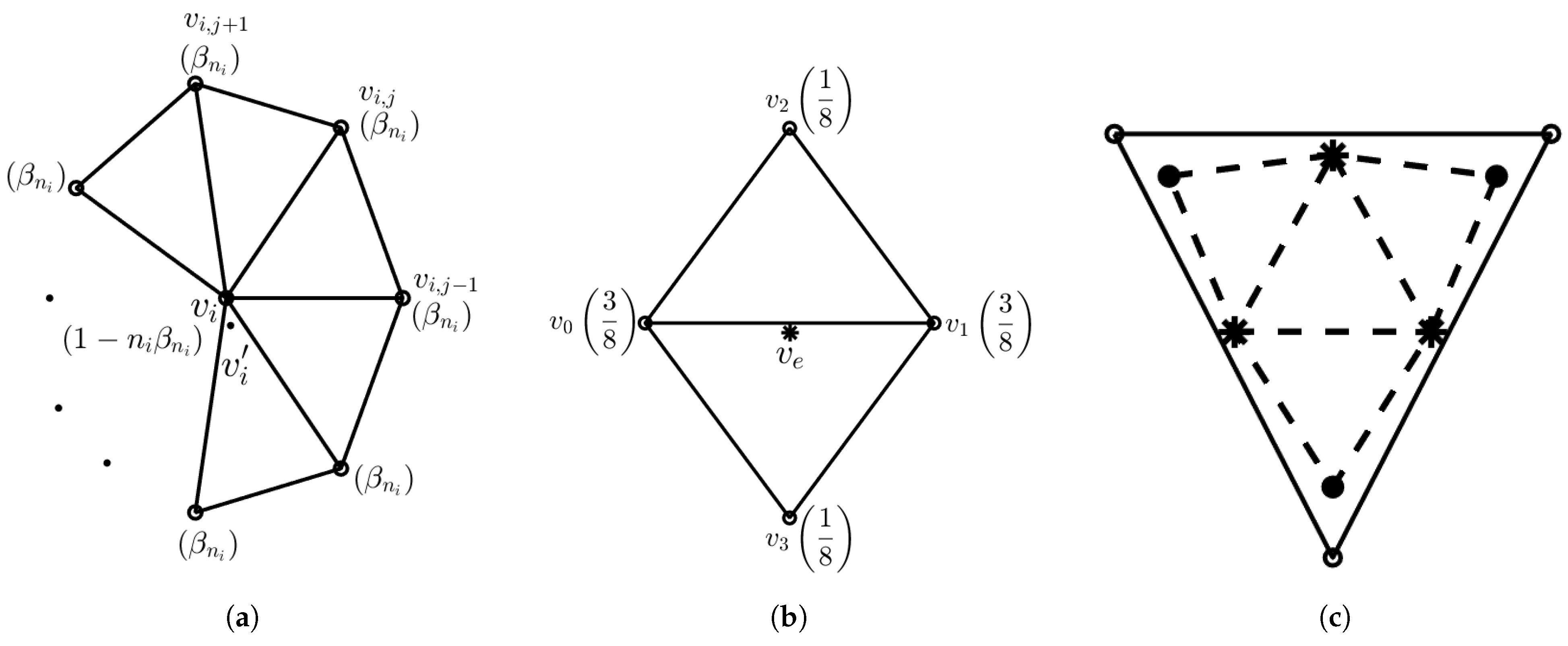
Assume that M is a triangular mesh, with a vertex set $V=\left\{v_i\right\}$ and an edge set $E=\left\{e_j\right\}$. The Loop subdivision rules are divided into two; the first rule is the geometry rule and the second rule is the topology rule. The geometry rule is the working procedure for generating new vertices, while the topology rule specifies the connections among the vertices.

1.

Generation of new vertex points: For an original vertex $v_i$ with valence $n_i$, the updated vertex $v_i^{\prime }$ is computed as

$$v_i^{\prime }=(1-n_i{\beta }_{n_i})v_i+{\beta }_{n_i}{\displaystyle \sum _{j=1}^{n_i}}{v}_{i,j},$$

(3)

where $v_{i,j}$ are the neighboring vertices of $v_i$, and

$${\beta }_{n_i}={\displaystyle \frac{1}{n_i}}\left({\displaystyle \frac{5}{8}}-{\left({\displaystyle \frac{3}{8}}+{\displaystyle \frac{1}{4}}cos{\displaystyle \frac{2\pi }{n_i}}\right)}^2\right).$$

See Figure 2a.

2.

Generation of new edge points: Consider two adjacent triangles $(v_0,v_1,v_2)$ and $(v_0,v_1,v_3)$ sharing the common edge $v_0{v}_1$ (see Figure 2b). The new edge point $v_e$ is defined as

$$v_e={\displaystyle \frac{3}{8}}(v_0+v_1)+{\displaystyle \frac{1}{8}}(v_2+v_3).$$

(4)

This edge-point computation rule is applied during each Loop subdivision refinement step to generate the refined triangular mesh and the corresponding smooth limit surface.

3.

Topological rules: Each newly computed vertex is connected to the surrounding new edge points, and neighboring edge points are also connected to produce the refined mesh, (see Figure 2c).

The repeated application of these rules produces a sequence of refined meshes converging to a smooth Loop subdivision surface.

3.2. Limit Point of Loop Subdivision Vertices

For a vertex $v_i$ with valence $n_i$, the limit position on the Loop subdivision surface denoted by $v_{i,\infty }$ is given by

$$v_{i,\infty }={\alpha }_{n_i}{v}_i+Q_i,$$

(5)

where

$${\alpha }_{n_i}={\displaystyle \frac{3}{11-8\left(\frac{3}{8}+{\left(\frac{3}{8}+\frac{1}{4}cos\frac{2\pi }{n_i}\right)}^2\right)}},Q_i={\displaystyle \frac{1-{\alpha }_{n_i}}{n_i}}\sum _j{v}_{i,j},$$

and $v_{i,j}$ are the vertices adjacent to $v_i$.

Let $V={[v_1,v_2,\dots ,v_m]}^T$ denote the vector of control vertices. The limit positions of all vertices can then be written in matrix form as

$$V_{\infty }=BV.$$

(6)

Here, B is the Loop subdivision limit matrix, defined as

$$B=\left(\begin{array}{cccc}{\alpha }_{n_1}& \dots & {\displaystyle \frac{1-{\alpha }_{n_1}}{n_1}}& \dots \\ ⋮& \ddots & ⋮& \\ {\displaystyle \frac{1-{\alpha }_{n_i}}{n_i}}& \dots & {\alpha }_{n_i}& \dots \\ ⋮& & & {\alpha }_{n_m}\end{array}\right).$$

(7)

Following [7], the matrix B admits the decomposition $B=\Gamma {\rm Y}$, where $\Gamma$ is a diagonal matrix with positive entries:

$$\Gamma =\left(\begin{array}{cccc}{\displaystyle \frac{1-{\alpha }_{n_1}}{n_1}}& 0& \dots & 0\\ 0& {\displaystyle \frac{1-{\alpha }_{n_2}}{n_2}}& \dots & 0\\ ⋮& & \ddots & ⋮\\ 0& \dots & & {\displaystyle \frac{1-{\alpha }_{n_m}}{n_m}}\end{array}\right),$$

(8)

and ${\rm Y}$ is a symmetric positive-definite (see [7] for more details):

$${\rm Y}=\left(\begin{array}{cccc}{\displaystyle \frac{n_1{\alpha }_{n_1}}{1-{\alpha }_{n_1}}}& \dots & 1& \dots \\ ⋮& \ddots & ⋮& \\ 1& \dots & {\displaystyle \frac{n_i{\alpha }_{n_i}}{1-{\alpha }_{n_i}}}& \dots \\ ⋮& \dots & & {\displaystyle \frac{n_m{\alpha }_{n_m}}{1-{\alpha }_{n_m}}}\end{array}\right).$$

(9)

Since $\Gamma$ is a diagonal matrix with strictly positive diagonal entries and ${\rm Y}$ is symmetric positive-definite, the matrix

$$B=\Gamma {\rm Y}$$

is also positive-definite. Moreover, the positivity of the subdivision weights together with the symmetric adjacency structure ensures that the resulting matrix satisfies the requirements of symmetric positive-definiteness. Consequently, the standard SOR convergence theory is applicable to the proposed SOR-PIA iteration. This matrix representation will play an essential role in the convergence analysis of the proposed algorithm. This matrix formulation will play a key role in the convergence analysis of the proposed SOR-PIA algorithm presented in Section 4.

3.3. Classical PIA for Loop Subdivision Surfaces

Let $M^{\left(0\right)}=(V,E)$ denote the initial mesh. After k iterations, the updated mesh is denoted by $M^{\left(k\right)}=(V^{\left(k\right)},E)$. The vector of Loop subdivision limit positions corresponding to the control mesh after the k-th iteration is denoted by $V_{\infty }^k$ and is given by

$$V_{\infty }^{\left(k\right)}=B{V}^{\left(k\right)}.$$

This classical PIA process can be interpreted as a stationary iterative method for solving the linear system

$$BV=V^{\left(0\right)},$$

where $V^{\left(0\right)}$ denotes the vector of original given mesh vertices. The difference vector between the original vertices and the current limit positions is defined as

$$d^{\left(k\right)}=V^{\left(0\right)}-V_{\infty }^{\left(k\right)}.$$

(10)

The new vertex $V^{(k+1)}$ is obtained according to the classical PIA scheme:

$$V^{(k+1)}=V^{\left(k\right)}+d^{\left(k\right)}.$$

(11)

To improve convergence, Weighted PIA (W-PIA) introduces a relaxation parameter $\sigma$:

$$V^{(k+1)}=V^{\left(k\right)}+\sigma d^{\left(k\right)}.$$

(12)

Additional PIA-based subdivision interpolation methods can be found in [9,10,11].

4. Methods

This section introduces the proposed Successive Overrelaxation–Progressive Iterative Approximation (SOR-PIA) technique for interpolating Loop subdivision surfaces. The essence is that the method iteratively adjusts the control mesh so that the limit surface of the Loop subdivision scheme interpolates the vertices of the initially given mesh.

Let $M=(V,E)$ represent the original mesh, where

$$V={\left\{v_i^0\right\}}_{i=0}^m$$

is the set of vertices, and

$$E={\left\{e_j\right\}}_{j=0}^n$$

is the set of edges.

At the initial step, we set $M^0=M$. The limit position of a vertex $v_i^0$, represented by $v_{i,\infty }^0$, is calculated using Equation (5). The equivalent difference vector is defined as

$$d_0^0={\displaystyle \frac{v_0^0-v_{0,\infty }^0}{{\alpha }_{n_0}}}.$$

(13)

The vertex $v_0^0$ is then updated using the SOR relaxation parameter $\omega \in (0, 2)$:

$$v_0^1=v_0^0+\omega d_0^0.$$

(14)

Let $V_i^0$ be the vertices of the control mesh $M_i^0$ define as $V_i^0=\{v_0^1,v_1^1,\cdots ,v_{i-1}^1,v_i^0,\cdots$, $v_m^0{\}}_{i=0}^m$. The limit point $v_{i,\infty }^0$ of $v_i^0$ on $M_i^0$ is computed as

$$v_{i,\infty }^0={\alpha }_{n_i}{v}_i^0+Q_i^0,$$

(15)

The difference vector $d_i^0$ and the updated vertex $v_i^1$ is, respectively, obtained in the same way as follows:

$$d_i^0={\displaystyle \frac{v_i^0-v_{i,\infty }^0}{{\alpha }_{n_i}}},v_i^1=v_i^0+\omega d_i^0.$$

(16)

When $i=m$ all vertices have been updated and the mesh $M^1$ has vertices $V^1={\left\{v_i^1\right\}}_{i=0}^m,$ where

$$v_i^1=v_i^0+\omega d_i^0,i=0,1,2,\cdots ,m.$$

Now the first iteration is completed.

Assume that, after the k-th SOR-PIA iteration, the control mesh is expressed by $M^k$ with vertex set

$$V^k={\left\{v_i^k\right\}}_{i=0}^m.$$

The limit position of vertex $v_i^k$ is given by

$$v_{i,\infty }^k={\alpha }_{n_i}{v}_i^k+Q_i^k.$$

The corresponding difference vector is calculated as

$$d_i^k={\displaystyle \frac{v_i^0-v_{i,\infty }^k}{{\alpha }_{n_i}}},i=0,1,2,\cdots ,m.$$

(17)

The new vertex $v_i^{k+1}$ is then expressed using SOR-PIA update rule as

$$\begin{array}{cc}\hfill v_i^{k+1}& =v_i^k+\omega d_i^k\hfill \\ \hfill & ={\displaystyle \frac{{\alpha }_{n_i}{v}_i^k+\omega v_i^0-\omega v_{i,\infty }^k}{{\alpha }_{n_i}}}\hfill \\ \hfill & ={\displaystyle \frac{(1-\omega ){\alpha }_{n_i}{v}_i^k+\omega (v_i^0-Q_i^k)}{{\alpha }_{n_i}}}\hfill \\ \hfill & =(1-\omega )v_i^k+{\displaystyle \frac{\omega }{{\alpha }_{n_i}}}(v_i^0-Q_i^k).\hfill \end{array}$$

(18)

In this manner, a sequence of control meshes

$${\left\{M^k\right\}}_{k=0}^{\infty }$$

is generated. In the next subsection, it is proved that the sequence converges to a limit mesh $M^{\infty }$, whose Loop subdivision surface interpolates the vertices of the original mesh.

Convergence of the SOR–PIA Algorithm for Loop Subdivision Surfaces

Let $V^k={[v_0^k,v_1^k,\dots ,v_m^k]}^T$ represent the vertex vector found after the k-th SOR-PIA iteration. Comparable to Equation (6), the subsequent limit positions can be written in matrix form as

$$V_{\infty }^k=B{V}^k,$$

(19)

where B is the Loop subdivision limit matrix defined in Equation (7). Using the decomposition $B=D-L-U$, where $D,L,$ and U denote the diagonal, strictly lower triangular, and strictly upper triangular parts of B, respectively, the term $Q_i^{\left(k\right)}$ can be represented collectively in matrix form through the neighboring vertex contributions contained in $L{V}^{(k+1)}+U{V}^{\left(k\right)}$. Consequently, the vertex-wise update relation in Equation (18) can be rewritten in matrix form as Equation (20).

From Equation (18), the SOR–PIA iteration can be expressed in matrix form as

$$V^{k+1}=(1-\omega )V^k+\omega D^{-1}\left(V^0+L{V}^{k+1}+U{V}^k\right),$$

(20)

Rearranging Equation (20) yields

$$\begin{array}{cc}\hfill V^{k+1}& ={(D-\omega L)}^{-1}\left[(1-\omega )D+\omega U\right]V^k+\omega {(D-\omega L)}^{-1}{V}^0,\hfill \\ \hfill & k=0,1,2,\dots .\hfill \end{array}$$

(21)

Define the iteration matrix

$${\mathcal{L}}_{\omega }={(D-\omega L)}^{-1}\left[(1-\omega )D+\omega U\right],I_{\omega }=\omega {(D-\omega L)}^{-1}.$$

Then, Equation (21) becomes

$$V^{k+1}={\mathcal{L}}_{\omega }{V}^k+I_{\omega }{V}^0,k=0,1,2,\dots .$$

(22)

Here, ${\mathcal{L}}_{\omega }$ is the SOR–PIA iteration matrix. Let $\rho \left({\mathcal{L}}_{\omega }\right)$ denote its spectral radius. It is well known that SOR iteration converges if $0<\omega <2$.

Theorem 1

([25]). Let $A=D-L-U$ be an $m\times m$ Hermitian matrix, where D is positive-definite. If $D-\omega L$ is nonsingular for $0\le \omega \le 2$, then the SOR iteration converges if and only if A is positive-definite and $0<\omega <2$.

Corollary 1

([25]). Let A be the coefficient matrix of the linear system $Ax=b$. Suppose that $A=D-L-U$ is an $n\times n$ Hermitian matrix with D positive-definite. Then, the block-successive overrelaxation method,

$$(D-\omega L)x^{k+1}=\left((1-\omega )D+\omega U\right)x^k+\omega b$$

, is convergent for any initial vector $x^0$ if, and only if, $0<\omega <2$ and A are positive-definite.

Theorem 2.

The SOR–PIA interpolation process for Loop subdivision surfaces is convergent.

Proof. 

From Section 3.2, the Loop subdivision limit matrix admits the decomposition

$$B=\Gamma {\rm Y},$$

where ${\rm Y}$ is symmetric positive-definite [7]. Since $\Gamma$ is a diagonal matrix with strictly positive entries and ${\rm Y}$ is symmetric positive-definite, the matrix B is also symmetric positive-definite. Consequently, the SOR iteration applied to the linear system

$$BV=V^{\left(0\right)}$$

satisfies the standard convergence conditions for symmetric positive-definite systems. Therefore, the SOR-PIA iteration defined in Equation (22) is convergent for any relaxation parameter $0<\omega <2$.

$\Gamma$ is a diagonal matrix with strictly positive values and ${\rm Y}$ is a symmetric positive-definite matrix, and B is a symmetric positive-definite matrix. Therefore, the SOR process of the linear system $BV=V^{\left(0\right)}$ meets the classical convergence criteria of symmetric positive-definite systems. Thus, for any relaxation parameter $0<\omega <2$, the SOR-PIA iteration given in Equation (22) is convergent.

By Theorem 1 and the classical SOR convergence theory [26], it follows that

$$\rho \left({\mathcal{L}}_{\omega }\right)<1,0<\omega <2.$$

Thus, the SOR-PIA iteration described in Equation (22) converges, and the sequence of control meshes produced by the algorithm converges to a limit mesh whose Loop subdivision surface interpolates the original mesh vertices. □

Remark 1

([26]). [Optimal relaxation parameter ω] For symmetric positive-definite matrices, the optimal relaxation parameter for the SOR iteration is given by

$$\omega ={\displaystyle \frac{2}{1+\sqrt{1-{\rho }^2(I_n-D^{-1}B)}}},$$

(23)

where $\rho (·)$ denotes the spectral radius, $I_n$ is the identity matrix, and B is symmetric positive-definite. This is the case when B is symmetric positive-definite.

In practical applications, the spectral radius is numerically approximated using a limited number of power-method iterations applied to the iteration matrix. Owing to the sparse and structured nature of Loop subdivision matrices, the computational expense of this estimation remains relatively small, even for moderately large mesh models. Moreover, the relaxation parameter can be determined once prior to the interpolation procedure and subsequently reused throughout the simulation process. The corresponding values of $\omega$ are presented in

Table 1. Number of iterations required for Loop surface interpolation for the mesh models shown in Figure 4.

Model	$\mathit{\omega }$	Method	${10}^{-1}$	${10}^{-2}$	${10}^{-3}$	${10}^{-4}$	${10}^{-5}$	${10}^{-6}$	${10}^{-7}$	${10}^{-8}$	${10}^{-9}$	${10}^{-10}$	CPU Time (s)
Ninja-Turtle	$1.9778$	PIA	1	5	12	19	27	35	43	51	60	68	1.8479
		W-PIA	1	4	8	12	17	22	26	31	36	41	1.1929
		HSS-PIA	1	3	7	11	16	20	25	29	34	39	1.7789
		WHSS-PIA	1	2	4	7	9	11	14	16	18	21	0.8774
		SOR-PIA	-	-	1	3	4	6	7	9	11	13	0.6265
Pumpkin	$1.9453$	PIA	1	6	13	20	28	36	43	51	59	67	3.0395
		W-PIA	1	4	8	12	16	21	26	30	35	40	1.8481
		HSS-PIA	1	4	8	12	16	20	25	29	34	38	2.6126
		WHSS-PIA	1	2	4	6	8	10	12	14	17	19	1.4453
		SOR-PIA	-	-	1	3	5	7	9	11	13	15	1.2002
Kangaroo	$1.9778$	PIA	1	6	16	26	37	48	60	71	83	95	2.7521
		W-PIA	1	3	7	12	17	22	27	32	37	43	1.5205
		HSS-PIA	1	4	9	15	21	26	33	40	46	52	2.2476
		WHSS-PIA	1	2	5	8	10	13	16	18	21	24	1.0606
		SOR-PIA	-	1	2	4	6	7	9	11	13	24	0.8122

.

The proposed SOR-PIA algorithm primarily stores sparse subdivision matrices together with vertex coordinate vectors. As a result, the memory requirement increases approximately linearly with the number of mesh vertices. Due to the sparsity of the Loop subdivision matrices, the proposed method remains memory-efficient even for comparatively dense meshes.

5. Results and Discussions

This section provides some numerical illustrations to show the effectiveness and efficiency of the proposed SOR-PIA in the interpolation of a Loop subdivision surface. Following all the examples, the red points are the original vertices of the initially given mesh, and the blue points are the control vertices modified by the SOR-PIA algorithm.

All iterative methods considered in this study were terminated when the relative fitting error satisfied

$${\displaystyle \frac{E_k}{E_0}}<\epsilon ,$$

where $E_k={max}_i∥v_i^{\left(0\right)}-v_{i,\infty }^{\left(k\right)}∥$ is the maximum variance between the original mesh vertices and their subdivision limit positions after k iterations, and $\epsilon$ is a tolerance. The same stopping strategy was used throughout SOR-PIA and all the comparison methods, so that the convergence performance can be fairly evaluated. In all experiments, the stopping tolerance was selected as $\epsilon ={10}^{(-10)}$ unless otherwise stated.

5.1. Interpolation Behavior of SOR-PIA

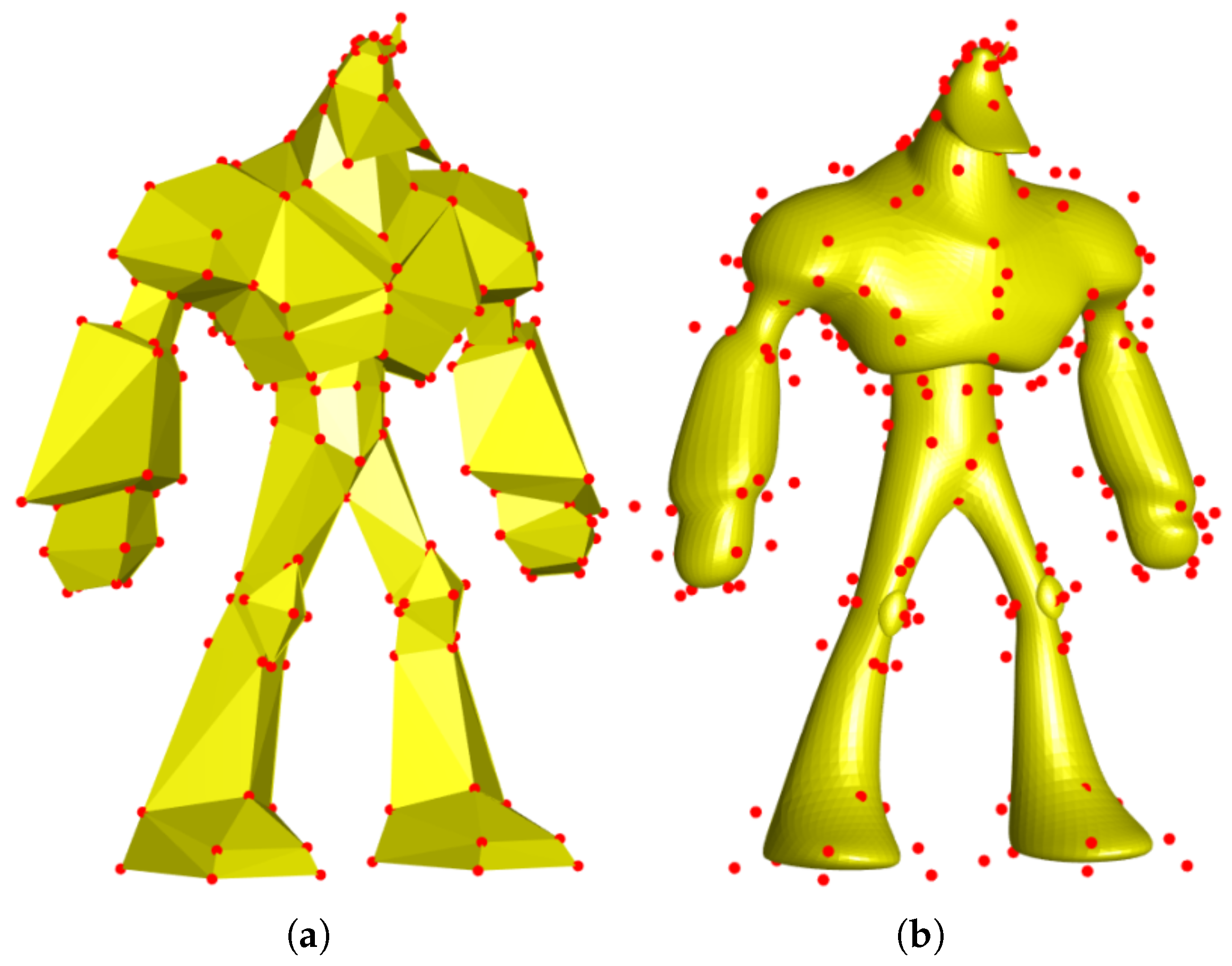
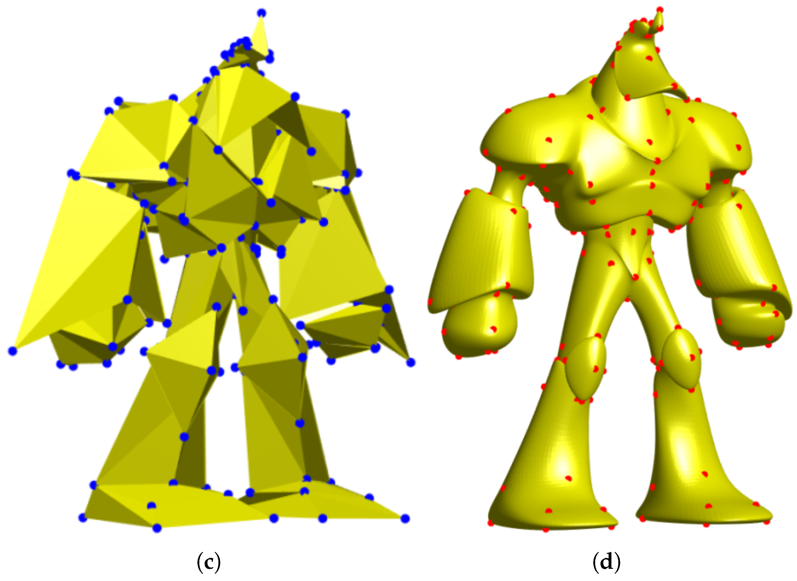
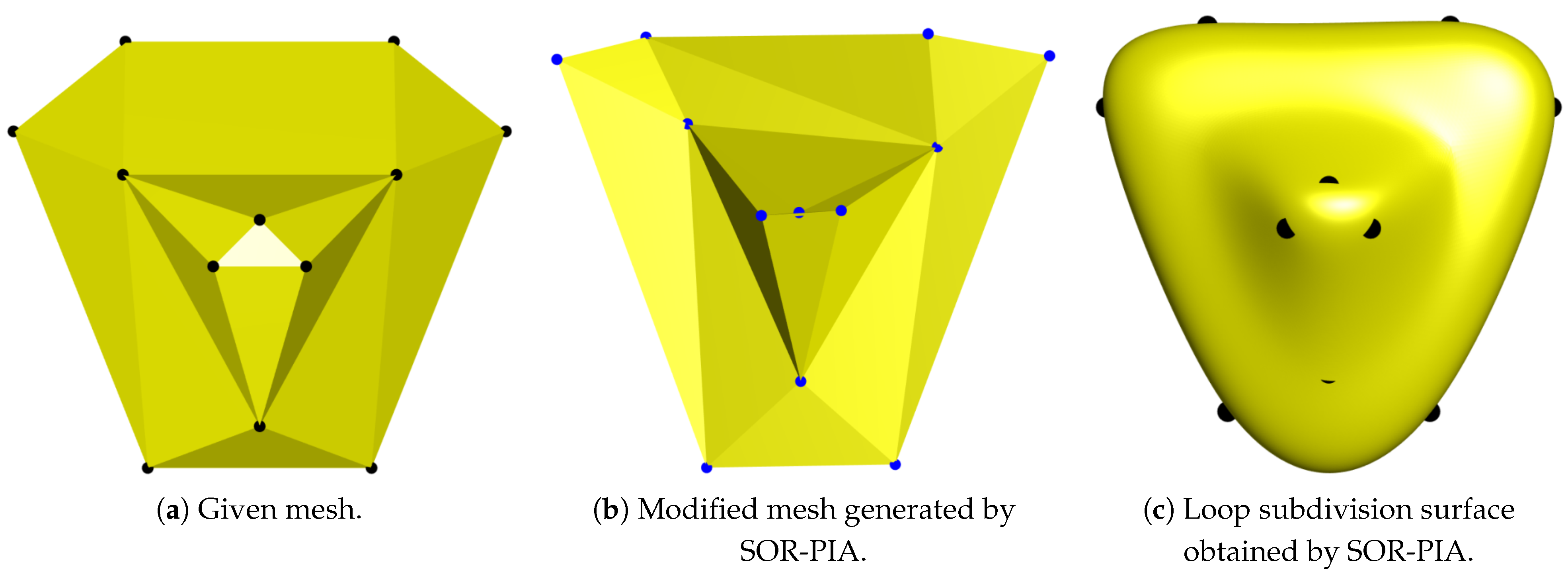
Figure 3 shows the disparity between the classical Loop subdivision surface and the surface obtained with the proposed SOR-PIA method. Figure 3a illustrates the mesh provided, which is the original. Figure 3b shows the Loop subdivision surface generated by the original mesh. Figure 3c represents the control mesh that is modified after five SOR-PIA iterations. The resultant Loop subdivision limit surface created using the modified mesh is shown in Figure 3d. The modified control mesh produced by the proposed SOR-PIA method effectively compensates for the shrinkage behavior associated with the classical Loop subdivision scheme. Consequently, the resulting subdivision surface approaches the original mesh vertices more closely while maintaining surface smoothness. This indicates that the proposed iterative correction strategy improves interpolation accuracy without introducing noticeable geometric artifacts. Furthermore, the surface generated using SOR-PIA (Figure 3d) preserves the shape characteristics of the original mesh more effectively and exhibits sharper geometric features compared with the classical Loop subdivision surface shown in (Figure 3b).

5.2. Surface Interpolation on Complex Mesh Models

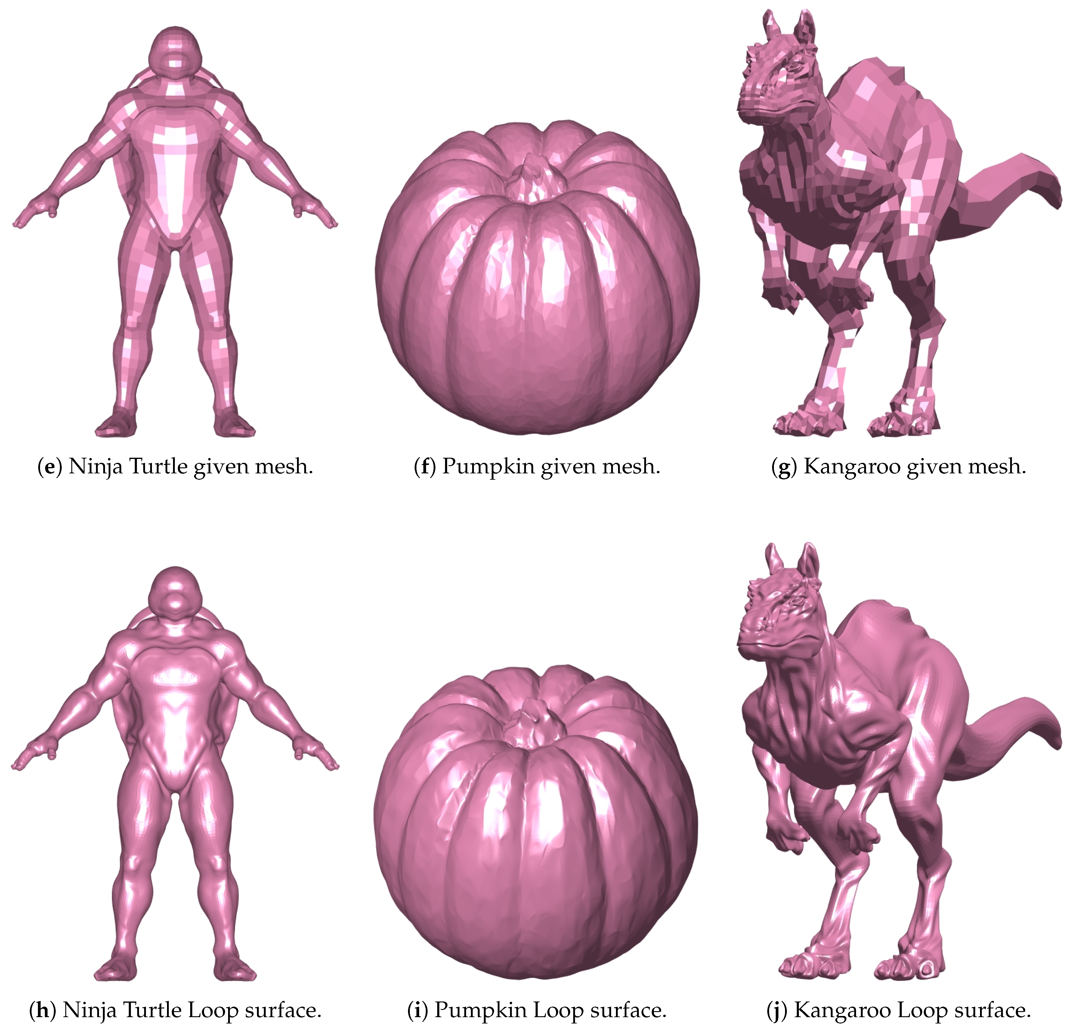
In order to further prove the strength of the proposed approach, three complicated mesh models are addressed: Ninja Turtle, Pumpkin, and Kangaroo. These models have varied mesh resolutions, with which the performance of the proposed method can be assessed. The original meshes are presented in the first row of Figure 4 and the respective interpolated Loop subdivision surfaces obtained by the SOR-PIA method are presented in the second row. The results obtained for the Ninja Turtle, Pumpkin, and Kangaroo models indicate that the proposed SOR-PIA approach remains robust and effective for meshes with varying geometric complexities and resolutions. The generated subdivision surfaces preserve the dominant geometric characteristics of the original models while providing improved interpolation performance compared with the classical Loop subdivision surface. For all three test models, the surfaces generated by SOR-PIA exhibit closer agreement with the original meshes.

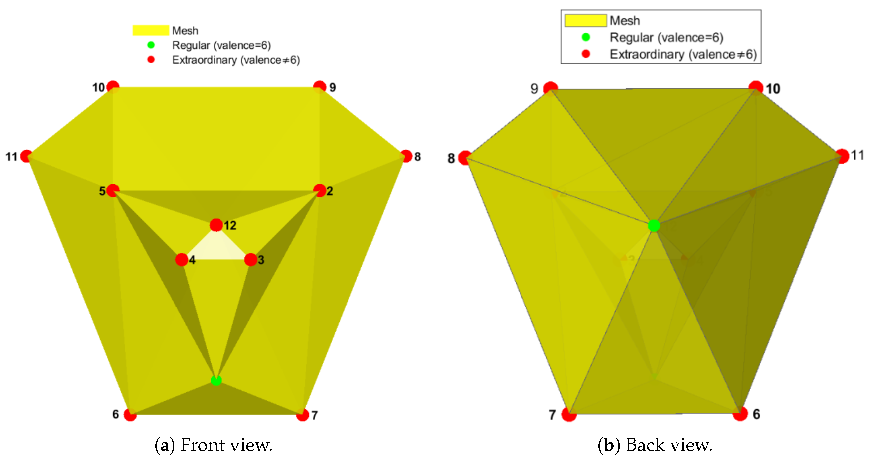
To further examine the robustness of the proposed approach, an additional experiment was performed using the Costa model (see Figure 5 and Figure 6), which contains a large number of extraordinary vertices with highly irregular valences (see

Table 2. Balance of the vertices of Costa model presented in Figure 5.

Vertex	1	2	3	4	5	6	7	8	9	10	11	12	13
Valence	6	8	4	4	7	5	5	4	4	5	4	4	6

). The obtained results show that the proposed method maintains stability and generates smooth subdivision surfaces even under severe topological irregularities (see Figure 6).

5.3. Convergence Performance Comparison

In order to assess the effectiveness of the proposed approach, we compare the rate of convergence of the proposed SOR-PIA with classical PIA [7], PIA with weights (W-PIA) [8], HSS-PIA [11], and WHSS-PIA [11].

Table 1 reports the number of iterations required for each method to satisfy the relative error criteria

$${\displaystyle \frac{E_k}{E_0}}<{10}^{-1},{10}^{-2},\dots ,{10}^{-10}.$$

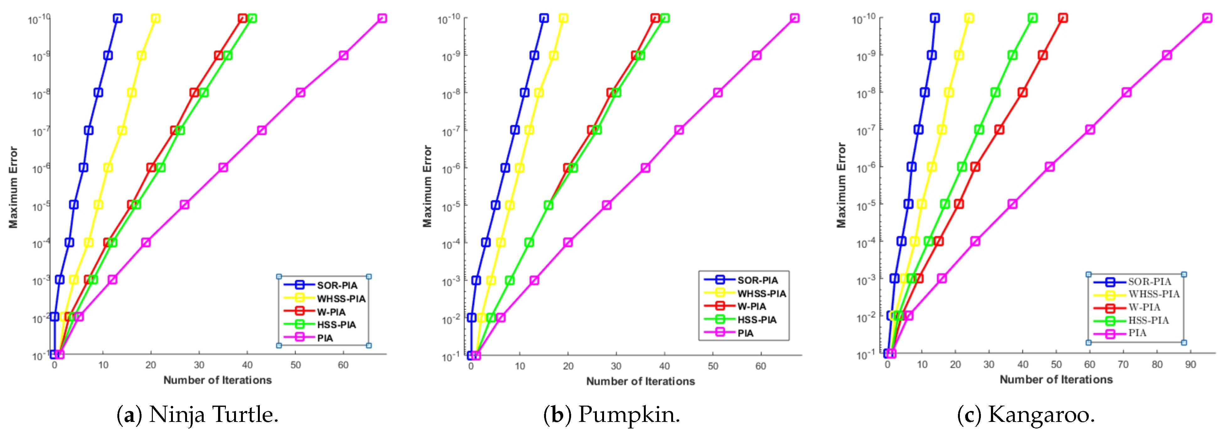
To further show the convergence performance, Figure 7 plots the fitting error versus the number of iterations for the several approaches applied to the three mesh models.

Based on Table 1 and Figure 7, it can be observed that the proposed SOR-PIA method always requires fewer iterations compared to classical PIA, W-PIA, HSS-PIA, and WHSS-PIA to attain the same level of accuracy. This proves the fact that the use of the successive overrelaxation technique highly boosts the convergence rate of PIA for Loop subdivision interpolation. As shown in Figure 4, it is evident that the proposed SOR-PIA method can generate smooth subdivision surfaces with a geometric shape similar to the original meshes. The interpolated surfaces produced by SOR-PIA faithfully reproduce the shapes of the original mesh models.

Table 1 shows that the proposed SOR-PIA method consistently attains the prescribed error tolerances using considerably fewer iterations than the competing approaches. The improvement becomes more pronounced for stricter tolerances, particularly for the Kangaroo model, where the classical PIA method requires 95 iterations to achieve an accuracy of ${10}^{-10}$ whereas SOR-PIA converges within only 24 iterations. The convergence curves presented in Figure 7 further demonstrate that SOR-PIA achieves a faster error decay rate, indicating a substantially accelerated convergence process. This enhancement is mainly attributed to the incorporation of the SOR relaxation strategy, which effectively decreases the spectral radius of the iteration matrix.

The final column of Table 1 reports the CPU execution time required by each method to attain the same accuracy level of ${10}^{-10}$. The timing results indicate that the accelerated convergence performance of SOR-PIA also contributes to lower computational cost. Although the SOR update step introduces additional arithmetic operations per iteration, the significant reduction in the overall number of iterations offsets this additional computational overhead.

6. Conclusions

This paper has proposed a novel progressive interpolation method for Loop subdivision surfaces on the basis of the successive overrelaxation (SOR) iterative method. In the proposed SOR-PIA algorithm, the control mesh is modified in such a manner that the limit surface produced by the Loop subdivision scheme interpolates the vertices of the initially provided mesh. The given method is much faster than classical PIA and its variations in terms of the convergence of the process of progressive interpolation. Theoretical analysis has determined the convergence of the SOR-PIA algorithm in the normal SOR conditions. A formula for the optimal relaxation parameter was also given to lead to practical implementation. Numerical results with various models of complex meshes showed that the proposed method is not only capable of producing interpolation but also of preserving geometric features, more than the classical Loop subdivision scheme. Furthermore, the SOR-PIA method always had fewer iterations to achieve the same error tolerance compared to PIA, W-PIA, HSS-PIA, and WHSS-PIA, which confirms its high level of effectiveness. Although the proposed method demonstrates promising convergence characteristics, several limitations still exist. In particular, determining the optimal relaxation parameter may become more difficult for extremely large-scale mesh models, and the current formulation is mainly developed for stationary Loop subdivision surfaces. Furthermore, the present study primarily emphasizes interpolation accuracy and convergence efficiency rather than real-time rendering applications. Future work will therefore focus on adaptive relaxation techniques, parallel GPU-based implementations, and the extension of the proposed framework to non-stationary and learning-assisted subdivision schemes.

References

- Dyn, N.; Levine, D.; Gregory, J.A. A butterfly subdivision scheme for surface interpolation with tension control. ACM Trans. Graph. 1990, 9, 160–169. [Google Scholar] [CrossRef] [Scilit]
- Zorin, D.; Schröder, P.; Sweldens, W. Interpolating subdivision for meshes with arbitrary topology. In Proceedings of the 23rd Annual Conference on Computer Graphics and Interactive Techniques (SIGGRAPH ’96), New Orleans, LA, USA, 4–9 August 1996; pp. 189–192. [Google Scholar]
- Kobbelt, L. Interpolatory subdivision on open quadrilateral nets with arbitrary topology. Comput. Graph. Forum 1996, 15, 409–420. [Google Scholar] [CrossRef] [Scilit]
- Loop, C. Smooth Subdivision Surfaces Based on Triangles. Master’s Thesis, University of Utah, Salt Lake City, UT, USA, 1987. [Google Scholar]
- Catmull, E.; Clark, J. Recursively generated B-spline surfaces on arbitrary topological meshes. Comput.-Aided Des. 1978, 10, 350–355. [Google Scholar] [CrossRef] [Scilit]
- Chen, Z.; Luo, X.; Tan, L.; Ye, B.; Chen, J. Progressive interpolation based on Catmull–Clark subdivision surfaces. Comput. Graph. Forum 2008, 27, 1823–1827. [Google Scholar] [CrossRef] [Scilit]
- Cheng, F.-H.; Fan, F.-T.; Lai, S.-H.; Huang, C.-L.; Wang, J.-X.; Yong, J.-H. Loop subdivision surface based progressive interpolation. J. Comput. Sci. Technol. 2009, 24, 39–46. [Google Scholar] [CrossRef] [Scilit]
- Deng, C.; Ma, W. Weighted progressive interpolation of Loop subdivision surfaces. Comput.-Aided Des. 2012, 44, 424–431. [Google Scholar] [CrossRef] [Scilit]
- Hamza, Y.F.; Lin, H. Conjugate-gradient progressive-iterative approximation for Loop and Catmull–Clark subdivision surface interpolation. J. Comput. Sci. Technol. 2022, 37, 487–504. [Google Scholar] [CrossRef] [Scilit]
- Wang, Z.; Li, Y.; Liu, J.; Ma, W.; Deng, C. Gauss–Seidel progressive iterative approximation (GS-PIA) for subdivision surface interpolation. Vis. Comput. 2023, 39, 139–148. [Google Scholar] [CrossRef] [Scilit]
- Hamza, Y.F.; Hamza, M.F.; Rababah, A.; Rano, S.A. HSS-progressive interpolation for Loop and Catmull–Clark subdivision surfaces. Sci. Afr. 2024, 23, e02070. [Google Scholar] [CrossRef] [Scilit]
- Zhang, B.; Zhang, Y.; Zheng, H. A symmetric non-stationary Loop subdivision with applications in initial point interpolation. Symmetry 2024, 16, 379. [Google Scholar] [CrossRef] [Scilit]
- Zhou, J.; Boonstra, J.; Kosinka, J. Subdivision shading for Catmull–Clark and Loop subdivision surfaces with semi-sharp creases. Computers 2023, 12, 85. [Google Scholar] [CrossRef] [Scilit]
- Liang, Y.; He, F.; Zeng, X.; Luo, J. An improved Loop subdivision to coordinate smoothness and number of faces via multi-objective optimization. J. Comput. Inf. Syst. 2022, 29, 1–10. [Google Scholar] [CrossRef] [Scilit]
- Liu, H.-T.D.; Kim, V.G.; Chaudhuri, S.; Aigerman, N.; Jacobson, A. Neural subdivision. ACM Trans. Graph. 2020, 39, 124. [Google Scholar] [CrossRef] [Scilit]
- Bandara, K.; Cirak, F. Subdivision surfaces in isogeometric analysis for shell structures. arXiv 2021, arXiv:2105.09288. [Google Scholar]
- Lin, H.; Bao, H.; Wang, G. Totally positive bases and progressive iteration approximation. Comput. Math. Appl. 2005, 50, 575–586. [Google Scholar] [CrossRef] [Scilit]
- Deng, C.; Lin, H. Progressive and iterative approximation for least squares B-spline curve and surface fitting. Comput.-Aided Des. 2014, 47, 32–44. [Google Scholar] [CrossRef] [Scilit]
- Jiang, Y.; Lin, H. IG-LSPIA: Least squares progressive iterative approximation for isogeometric collocation method. Mathematics 2023, 11, 898. [Google Scholar] [CrossRef] [Scilit]
- Shou, H.; Hu, L.; Fang, S. Progressive iterative approximation of non-uniform cubic B-spline curves and surfaces via successive over-relaxation iteration. Mathematics 2022, 10, 3766. [Google Scholar] [CrossRef] [Scilit]
- Hamza, Y.F.; Jiang, Y.; Lin, H. Gauss–Seidel progressive and iterative approximation for least squares fitting. J. Comput.-Aided Des. Comput. Graph. 2021, 33, 1–10. [Google Scholar]
- Hamza, Y.F.; Lin, H.; Li, Z. Implicit progressive-iterative approximation for curve and surface reconstruction. Comput. Aided Geom. Des. 2020, 77, 101829. [Google Scholar] [CrossRef] [Scilit]
- Jiang, Y.; Lin, H.; Huang, W. Fairing-PIA: Progressive-iterative approximation for fairing curve and surface generation. Vis. Comput. 2024, 77, 1467–1484. [Google Scholar]
- Lin, H.; Maekawa, T.; Deng, C. Survey on geometric iterative methods and their applications. Comput.-Aided Des. 2018, 95, 40–51. [Google Scholar]
- Varga, R.S. Matrix Iterative Analysis, 2nd ed.; Springer: Berlin/Heidelberg, Germany, 2009. [Google Scholar]
- Quarteroni, A.; Sacco, R.; Saleri, F. Numerical Mathematics; Springer: New York, NY, USA, 2000. [Google Scholar]