Improving Short-Term Gas Load Forecasting Accuracy: A Deep Learning Method with Dual Optimization of Dimensionality Reduction and Noise Reduction

Abstract

Accurate short-term (10–20 days) natural gas load forecasting is crucial for the “tactical planning” of gas utilities, yet it faces significant challenges from high volatility, strong noise, and the high-dimensional multicollinearity of influencing factors. To address these issues, this paper proposes a novel hybrid forecasting framework: PCCA-ISSA-GRU. The framework first employs Principal Component Correlation Analysis (PCCA), which improves upon traditional PCA by incorporating correlation analysis to effectively select orthogonal features most relevant to the load, resolving multicollinearity. Concurrently, an Improved Singular Spectrum Analysis utilizes statistical criteria (skewness and kurtosis) to adaptively separate signals from Gaussian noise, denoising the historical load sequence. Finally, the dually optimized data is fed into a Gated Recurrent Unit (GRU) neural network for prediction. Validated on real-world data from a large city in Northern China, the PCCA-ISSA-GRU model demonstrated superior performance. For a 20-day forecast horizon, it achieved a Mean Absolute Percentage Error (MAPE) of 6.09%. Results show its accuracy is not only significantly better than single models (BPNN, LSTM, GRU) and classic hybrids (ARIMA-ANN), but also outperforms the state-of-the-art (SOTA) model, Informer, within the 10–20 days tactical window. This superiority was confirmed to be statistically significant by the Diebold–Mariano test (p < 0.05). More importantly, the model exhibited exceptional robustness, with its error increase during extreme weather scenarios (e.g., cold waves, rapid temperature changes) being substantially lower (+56.7%) than that of Informer (+109.2%). The PCCA-ISSA-GRU framework provides a high-precision, highly robust, and cost-effective solution for urban gas short-term load forecasting, offering significant practical value for critical operational decisions and high-risk scenarios.

1. Introduction

1.1. Research Background

As the third global energy revolution progresses, the world’s energy system is undergoing a long and critical transition from traditional fossil fuels to renewable energy sources [1]. During this transformation, natural gas, owing to its relatively clean and efficient properties, is widely regarded as the “bridge fuel” connecting high-carbon energy sources with a zero-carbon future [2]. It plays a vital role in optimizing the global energy mix, reducing greenhouse gas emissions, and ensuring energy security [3]. Consequently, many nations are actively expanding the utilization of natural gas, driving a steady increase in its share of primary energy consumption.

In the current energy landscape, accurate natural gas load forecasting (NGLF) has become a critical technology for ensuring the economic and efficient operation of urban gas systems [4]. The global natural gas market is experiencing significant vulnerability, as geopolitical tensions and supply-side constraints exacerbate price volatility. Authoritative bodies, such as the International Energy Agency (IEA) and the U.S. Energy Information Administration (EIA), have persistently emphasized that the global natural gas balance remains delicate [5,6]. This uncertainty places immense pressure on gas utility companies, compelling them to optimize operational planning, manage inventories, and mitigate the financial risks arising from supply-demand imbalances.

A critical, yet frequently overlooked, challenge lies in the specific forecasting horizon. Planning for gas utilities is not monolithic; it is segmented by distinct time scales:

(1)

Operational Dispatch (<7 days): This horizon is primarily dictated by strict pipeline “Nomination Cycles” and typically requires “Day-ahead” or “Intra-day” forecasts for immediate scheduling [7].

(2)

Strategic Planning (>3 months): This scale involves long-term procurement and seasonal storage strategies, often guided by annual “Integrated Resource Planning” (IRPs) [8].

This paper addresses the critical “Tactical Planning Gap” that exists between these two horizons. Within this 10 to 20-day window, utilities must make high-stakes operational and financial decisions, such as scheduling storage withdrawals or procuring resources from the spot market to balance supply. Inaccurate forecasts during this period can lead to severe financial penalties or significant resource waste [9,10]. This study, therefore, selects a 10- to 20-day forecasting horizon specifically to provide decision-support tools for this tactical window.

Natural gas load forecasting (NGLF) is the process of predicting future gas demand over a specified period [11]. It involves utilizing historical load data, quantitatively analyzing various influencing factors—such as temperature, weather patterns, economic activity, and public holidays—and constructing mathematical models to uncover the underlying patterns in consumption. Given its significance, scholars and engineers worldwide have demonstrated considerable interest in this field, driving substantial advancements in forecasting theory and modeling methodologies [12,13].

1.2. Literature Review & Problem Identification

1.2.1. Traditional and AI Models

Short-term forecasting (on an hourly, daily, or weekly basis) is particularly critical for guiding the daily dispatch of gas companies, assessing transaction volumes, and formulating peak-shaving strategies. Research in this domain can be broadly categorized into three phases: the traditional model phase, the artificial intelligence (AI) model phase, and the hybrid model phase [14,15].

In the early stages of computational technology, research primarily relied on classical statistical and econometric models. For example, the Hubbert curve was used to describe the life cycle of resource production but exhibited significant errors when forecasting gas load during periods of economic fluctuation. Econometric methods, typified by the B&N model, began to incorporate external variables such as price, income, and weather, offering a new perspective on load forecasting [16]. Following advancements in computer technology, regression models (RM), time series (TS) models such as ARIMA, and grey models (GM) were applied [17]. These models, characterized by relatively simple structures, were capable of extracting trends from limited data and laid the theoretical foundation for load forecasting during that era. However, their capacity to handle the inherent non-linearity and high volatility characteristic of gas load data was limited, and their forecasting accuracy struggled to meet the demands of modern scheduling [18].

To overcome the limitations of traditional models, researchers turned to the field of artificial intelligence, developing models capable of effectively capturing non-linear relationships. Among these, Artificial Neural Networks (ANN) and Support Vector Regression (SVR) are the most representative techniques. ANNs, by emulating the structure of human neurons, demonstrated robust non-linear fitting capabilities [19]. SVR, based on the structural risk minimization (SRM) principle and the introduction of kernel functions, excelled in handling small-sample, high-dimensional data, effectively avoiding the local optima and overfitting issues prevalent in neural networks [20]. Extensive research confirmed that, compared to traditional models, ANNs and SVR achieved superior accuracy in short-term load forecasting tasks, signaling the advent of a new, data-driven, intelligent era for load forecasting [21,22].

1.2.2. Hybrid Models and Preprocessing

Since the early 21st century, with advancements in machine learning theory and the exponential growth in computational power, standalone models have become insufficient to meet the increasing demands for accuracy [23]. Consequently, natural gas load forecasting (NGLF) entered a comprehensive development phase characterized by “hybridization” and “deep learning.” Research during this period has exhibited several primary trends:

(1)

Data Decomposition Combined with Models: To address the non-stationarity and noise interference inherent in raw load sequences, researchers have widely adopted signal decomposition techniques, such as Wavelet Transform (WT), Empirical Mode Decomposition (EMD), and Variational Mode Decomposition (VMD). These methods decompose the complex original series into several more stationary and regular sub-sequences. Each sub-sequence is then forecasted separately, and the results are aggregated, significantly enhancing prediction accuracy [24,25].

(2)

Optimization Algorithms Combined with Models: To address the challenges of difficult parameter selection and susceptibility to local optima in predictive models (particularly ANNs and SVR), researchers have introduced swarm intelligence optimization algorithms, such as Particle Swarm Optimization (PSO), Grey Wolf Optimizer (GWO), and Harris Hawks Optimization (HHO) [26]. By employing these algorithms to automatically determine the optimal combination of model parameters, the performance and generalization capability of the models can be substantially enhanced.

Recent research has also emphasized the importance of performing data clustering prior to forecasting. In the energy domain, clustering algorithms (such as K-Means) are used not merely for simple grouping but are more frequently applied for “Load Profile Analysis” [27]. For instance, studies have utilized the K-Means algorithm to cluster industrial thermal loads based on their dependency on ambient temperature, which aligns with this paper’s emphasis on meteorological factors. Through clustering, heterogeneous data (such as different user types or seasons) can be partitioned into more homogeneous subsets, thereby enhancing the stability of subsequent AI models.

Furthermore, gas load data is often corrupted by discrete, non-physical outliers. Previous studies have employed density-based clustering algorithms such as DBSCAN for denoising purposes [28,29]. This differs from the “denoising” problem addressed by the ISSA algorithm in this paper (Section 2.2). DBSCAN captures large, isolated spikes, whereas ISSA (which is based on Singular Spectrum Analysis) is designed to identify and remove more widespread, approximately Gaussian random high-frequency “noise” by analyzing statistical properties (skewness and kurtosis).

1.2.3. SOTA Models: From RNN to Transformer

The Rise of Deep Learning Models: Deep learning (DL) models, typified by Long Short-Term Memory (LSTM), Gated Recurrent Unit (GRU), and Deep Belief Networks (DBN), have gained considerable favor due to their superior capability in handling long-term dependencies within time series data [30]. These models can more effectively learn complex dynamic patterns from historical data, establishing them as state-of-the-art (SOTA) predictive tools. However, despite the strong performance of LSTM and GRU, they still suffer from a sequential bottleneck, which hinders their ability to capture ultra-long-term dependencies. In recent years, models based on the Attention Mechanism have emerged as SOTA methods. The Transformer model [31] utilizes a Self-Attention mechanism, which permits the model to process sequences in parallel and directly capture dependencies between any two points in the sequence, demonstrating immense potential across multiple domains [32].

To address the computational complexity and memory bottlenecks of the standard Transformer when applied to Long-Series Time series Forecasting (LSTF) tasks, subsequent studies, such as the Informer, were proposed. The Informer introduced the ProbSparse Self-Attention mechanism, which significantly reduces the complexity from $O(L^2)$ to $O(L\log L)$ by sparsifying the attention weights through probabilistic sampling. Concurrently, it employs a “self-distilling” mechanism to progressively reduce the sequence length within the encoder, thereby efficiently extracting dominant features [33]. The Informer has demonstrated exceptional performance in energy-related tasks, including energy load forecasting [34]. A comparison of these advanced predictive models from the literature review is presented in

Table 1. Comparison of Advanced Predictive Models in the Literature Review.

Model	Core Mechanism	Advantages	Limitations
LSTM/GRU	Recurrent Gating Units	Efficient handling of temporal dependencies	Difficulty in capturing ultra-long-term dependencies; sequential computation
Transformer	Self-Attention	Parallel computation; strong long-term dependency capturing	$O(L^2)$ complexity; not suitable for extremely long sequences
Informer	ProbSparse Self-Attention	Complexity reduced to $O(L\log L)$; designed for long sequence forecasting	Complex structure; numerous hyperparameters

.

1.2.4. International Research and Regional Differences

Advancements in this field indeed exhibit strong regional contexts and divergent research focuses. In North America, researchers began using Deep Neural Networks (DNNs) for natural gas load forecasting in the U.S. Midwest relatively early, while recent studies have delved deeper into new challenges within the “electrification-decarbonization” paradigm. For instance, scholars have begun to concentrate on analyzing the coupled impacts of electric vehicle (EV) adoption and the large-scale replacement of traditional heating with heat pumps on the “gas-electric nexus” [35,36,37], which demands predictive models that transcend single-energy modalities.

In Europe, research is equally active: German studies focus on high-resolution, day-ahead supply and demand forecasting to cope with market volatility [38,39]; research targeting mature markets like the United Kingdom and the Netherlands has compared the performance of various advanced models, such as XGBoost, SSA, and LSTNet, across different time scales [40,41]. A notable recent trend since 2022 is the emergence of numerous studies urgently evaluating the impact of geopolitically induced price volatility on demand elasticity, as well as the challenges that supply uncertainty poses to short-term forecasting models [42,43,44].

Meanwhile, research in Asia, particularly in China, constitutes another significant branch. Unlike the mature markets of North America and Europe, China’s research priorities are often closely tied to rapid demand growth, the phased impacts of the large-scale “coal-to-gas” policy, and infrastructural constraints (such as LNG receiving terminals and pipeline network layouts) [45]. In terms of model application, besides mainstream deep learning models (like LSTM), Grey Models (GM) and their hybrid modified forms (e.g., ARIMA-GM or metabolic GM(1,1) models) still hold a significant position in China’s medium- and long-term aggregate demand forecasting, especially considering data availability limitations and abrupt policy shifts [46,47]. Furthermore, studies focusing on major LNG-importing countries like Japan and South Korea tend to concentrate more on the influence of global LNG spot prices, inventory strategies, and shifting nuclear power policies on their domestic demand [48,49].

1.2.5. Problem Identification and Contributions

Despite significant achievements by global scholars in the field of natural gas load forecasting, several challenges and limitations persist within the specific context of short-term load forecasting:

(1)

The “Information Misalignment” Defect in Feature Extraction Mechanisms: Traditional dimensionality reduction methods, such as Principal Component Analysis (PCA), rely primarily on variance maximization theory, prioritizing principal components with large eigenvalues. However, natural gas load forecasting presents a paradox of “low variance but high correlation.” Subtle meteorological changes or specific holiday factors, while statistically insignificant in terms of variance (corresponding to smaller eigenvalues), are highly correlated with load variations. Traditional PCA treats these features as “noise” and discards them. This sorting mechanism—based on variance rather than correlation—directly leads to the loss of critical predictive information. Although Kaib et al. (2023) [50] proposed an improved Kernel PCA based on fractal dimensions, this method is primarily designed for fault detection in non-linear industrial processes. It focuses on identifying abnormal states and lacks an explicit mechanism to reconstruct and rank features based on their “correlation with the prediction target,” making it unsuitable for directly resolving the issue of information loss in load forecasting.

(2)

Lack of Pertinence in Data Denoising: Short-term gas load series are characterized by high volatility and non-stationarity, containing significant noise caused by sudden user behaviors. Existing decomposition methods (e.g., EMD, VMD) often face challenges such as mode mixing or difficulty in parameter selection. While there is extensive research on improving Singular Spectrum Analysis (SSA)—such as the robust SSA proposed by Kazemi et al. (2025) [51] and the optimized SSA by Gupta (2025) [52]—these methods improve signal separation capabilities to a certain extent. However, most assume that noise follows a Gaussian distribution or rely on complex iterative optimization. Urban gas loads, aside from Gaussian noise, often exhibit non-Gaussian, high-skewness “spike” patterns. When handling such noise, existing methods tend to result in either excessive residual noise or over-smoothing, failing to restore the true fluctuation trend of the load.

(3)

Need for Improved Model Adaptability to Complex Features: Although deep learning models (such as LSTM and GRU) can effectively capture dynamic dependencies in time series, constructing a robust model that can adaptively learn features from multiple sub-sequences generated by complex decomposition remains a challenge [53]. Furthermore, while State-of-the-Art (SOTA) models like Transformer and Informer are powerful, they typically possess complex structures, require massive datasets, and demand fine-grained hyperparameter tuning and high computational power [32,33].

Therefore, investigating how to enhance the performance and robustness of lighter, deployable models (e.g., GRU) through advanced, domain-specific preprocessing techniques remains of significant academic value and application efficiency for the specific scenario of natural gas “tactical planning” (10–20 days) [54]. Given that PCA and SSA algorithms are characterized by clear structures and lightweight deployment, they are amenable to domain-specific tuning. Adhering to the principles of lightweight deployment and high predictive robustness, this study proposes a hybrid PCCA-ISSA-GRU (Principal Correlation Component Analysis-Improved Singular Spectrum Analysis-Gated Recurrent Unit) prediction model. This model adopts a strategy of “advanced domain-specific preprocessing + lightweight model” to achieve efficient natural gas load forecasting on low-computing power platforms and in specific scenarios, thereby addressing the issues faced by existing models in short-term forecasting.

2. Models & Methods

Short-term natural gas load forecasting (NGLF) is inherently a high-dimensional, large-data prediction problem. Both the volume of influencing factors and the length of the historical data series often exceed those of other forecasting types. This high dimensionality and large data volume not only impose a significant burden on predictive models but also amplify the overall complexity of the forecasting task [55]. Moreover, analyzing the impact of each factor individually would necessitate the design of numerous cross-combination scenarios, each requiring separate simulation. This approach unequivocally increases the analytical workload, while the practical utility of the method and the applicability of its results are severely limited.

Due to stochastic influences, historical NGLF data often contains numerous outliers. These outliers can interfere with the underlying patterns of the load data, disrupt the similarity of gas loads within the same period, and consequently degrade the model’s forecasting accuracy [56,57,58]. Addressing these outliers is therefore an essential preprocessing step.

To address the dual challenges of complex high-dimensional data processing and the presence of anomalous data, this study adopts an improved Principal Component Analysis algorithm (PCCA) for dimensionality reduction and key factor analysis. Concurrently, an improved Singular Spectrum Analysis algorithm (ISSA) is employed for data cleansing. Finally, these components are combined with a GRU neural network to form a hybrid forecasting model that integrates data analysis, preprocessing, and prediction. Overall, the proposed model utilizes a combination of improved, lightweight preprocessing algorithms and a lightweight predictive model to achieve efficient, rapid, and accurate short-term NGLF on low-computation platforms.

2.1. Improvement of the PCA Algorithm (PCCA)

2.1.1. Shortcomings of the PCA Algorithm in Gas Load Data Processing

The Principal Component Analysis (PCA) algorithm can transform several correlated variables into an equal number of uncorrelated components. By extracting the principal components from the data to replace the original dataset, it achieves the goal of reducing dataset dimensionality and eliminating redundant information. Utilizing the PCA algorithm to reduce the dimensionality of the original dataset retains the main data components while simultaneously reducing the input data dimensionality for the predictive model [59]. The PCA algorithm primarily involves three processes: mean centering and standardization, eigendecomposition, and reconstruction.

Although the PCA algorithm can extract the principal components of the original variables, its reconstruction process relies on ranking and filtering components based solely on the magnitude of their eigenvalues. This causes the linear relationship between each component and the target variable (natural gas load) to be disregarded, rendering the standard PCA process unsuitable for direct application in short-term NGLF [50].

The experimental data used is the gas load data from a large city in Northern China (identical to that used in subsequent forecasting experiments), with results shown in Figure 1. (In the figures, NG represents daily natural gas load, LT represents daily low temperature, AT represents daily average temperature, HT represents daily high temperature, LD represents daily low dew point, AD represents daily average dew point, and HD represents daily high dew point). Figure 1a shows the correlation heatmap of the original data, where temperature factors and dew point factors have a high correlation with natural gas load (all > 0.50). Concurrently, the correlation among these factors themselves is high (all > 0.80). In Figure 1b, which shows the principal components obtained by standard PCA, all components are uncorrelated variables, effectively reducing variable correlation and redundant input.

However, a critical issue is observed: the 4th component obtained by PCA has a correlation of only 0.01 with NG, whereas the 6th component has a correlation of 0.16. Although the eigenvalue of the 6th component is lower than that of the 4th, its correlation with NG is significantly higher. Therefore, if components are selected based on eigenvalue magnitude alone, it is highly probable that important components with high target correlation will be discarded in favor of components with low target correlation.

2.1.2. Introducing Correlation Analysis Correction to the PCA Algorithm

To address this issue, we propose an algorithm for processing influencing factors that is specifically tailored for short-term natural gas load forecasting. This method builds upon the traditional PCA algorithm by considering the correlation between each component and the natural gas load. It modifies the reconstruction process of PCA by introducing a correlation analysis step, thereby forming a new influencing factor processing algorithm, which we name Principal Component Correlation Analysis (PCCA).

The PCCA algorithm also comprises three stages: mean-centering and standardization, eigendecomposition, and reconstruction. The first two stages are identical to those of the standard PCA algorithm. However, in the reconstruction stage, after the eigenvector matrix U is obtained from eigendecomposition, a principal component matrix is formed. This matrix contains n principal components, where each component can be represented as $L_i=\left[L_{i,1},L_{i,2},L_{i,3}\dots L_{i,m}\right]$ for i = 1, 2, …, n. Let the daily natural gas load series be denoted by $Y=\left[y_1,y_2,\dots ,y_m\right]$. The direct correlation between each component and the daily load can then be calculated using Equations (1) and (2):

$$\mathrm{cov}(L_i,Y)={\displaystyle \frac{{\displaystyle \sum _{j=1}^m(L_{i,j}-\overline{L_i})(y_j-\overline{Y})}}{m-1}}$$

(1)

$${\rho }_{L_i,Y}={\displaystyle \frac{\left|\mathrm{cov}(L_i,Y)\right|}{\sqrt{D(L_i)D(Y)}}}$$

(2)

where $\mathrm{cov}(L_i,Y)$ is the covariance between component L_i and the load Y; $\overline{L_i}$ is the mean of L_i; $\overline{Y}$ is the mean of Y; $D(L_i)$ is the variance of L_i; D(Y) is the variance of Y;${\rho }_{L_i,Y}$ is the correlation coefficient between component L_i and the load Y, with its absolute value ranging from [0, 1], where 1 indicates perfect linear correlation and 0 indicates no linear correlation.

Subsequently, the correlation coefficients of all components are arranged in descending order, and the contribution rate of each component is calculated as shown in Equation (3):

$$p_i={\displaystyle \frac{{\rho }_{L_i,Y}}{{\displaystyle \sum _{i=1}^n{\rho }_{L_i,Y}}}}\times 100\%$$

(3)

where p_i is the contribution of component L_i.

A contribution threshold, S_P, is set within the range of 0% to 100%. We then select the top r components (where r < n) such that their cumulative contribution exceeds SP. Finally, the components corresponding to these selected contributions are extracted to serve as the input parameters for the forecasting model.

The results after processing with the PCCA algorithm are shown in Figure 2. Compared to the original PCA algorithm, the correlation of the new PCCA-derived features with the NG load is strictly monotonically decreasing, which provides a clear and meaningful ranking of information. Both methods perform consistently on the first three principal components. However, a significant divergence occurs at the 4th and 5th components: PCCA retains substantial correlation with NG (0.26 and 0.16, respectively), whereas the original PCA components lost nearly all relevant correlation (0.01 and 0.02). This demonstrates that the improved PCCA algorithm successfully retains more critical features relevant to the target variable.

2.2. Improvement of the SSA Algorithm (ISSA)

2.2.1. The Problem of Sub-Sequence Feature Loss in SSA

The Singular Spectrum Analysis (SSA) algorithm constructs a time-lag (trajectory) matrix from a time series of N samples based on a given embedding dimension. It then performs eigendecomposition (or Singular Value Decomposition, SVD) on this matrix to obtain eigenvalues and eigenvectors. The SSA algorithm can be broadly divided into two stages: Decomposition and Reconstruction. The Decomposition stage includes Embedding and Eigendecomposition; the Reconstruction stage includes Grouping, Diagonal Averaging, and Selection.

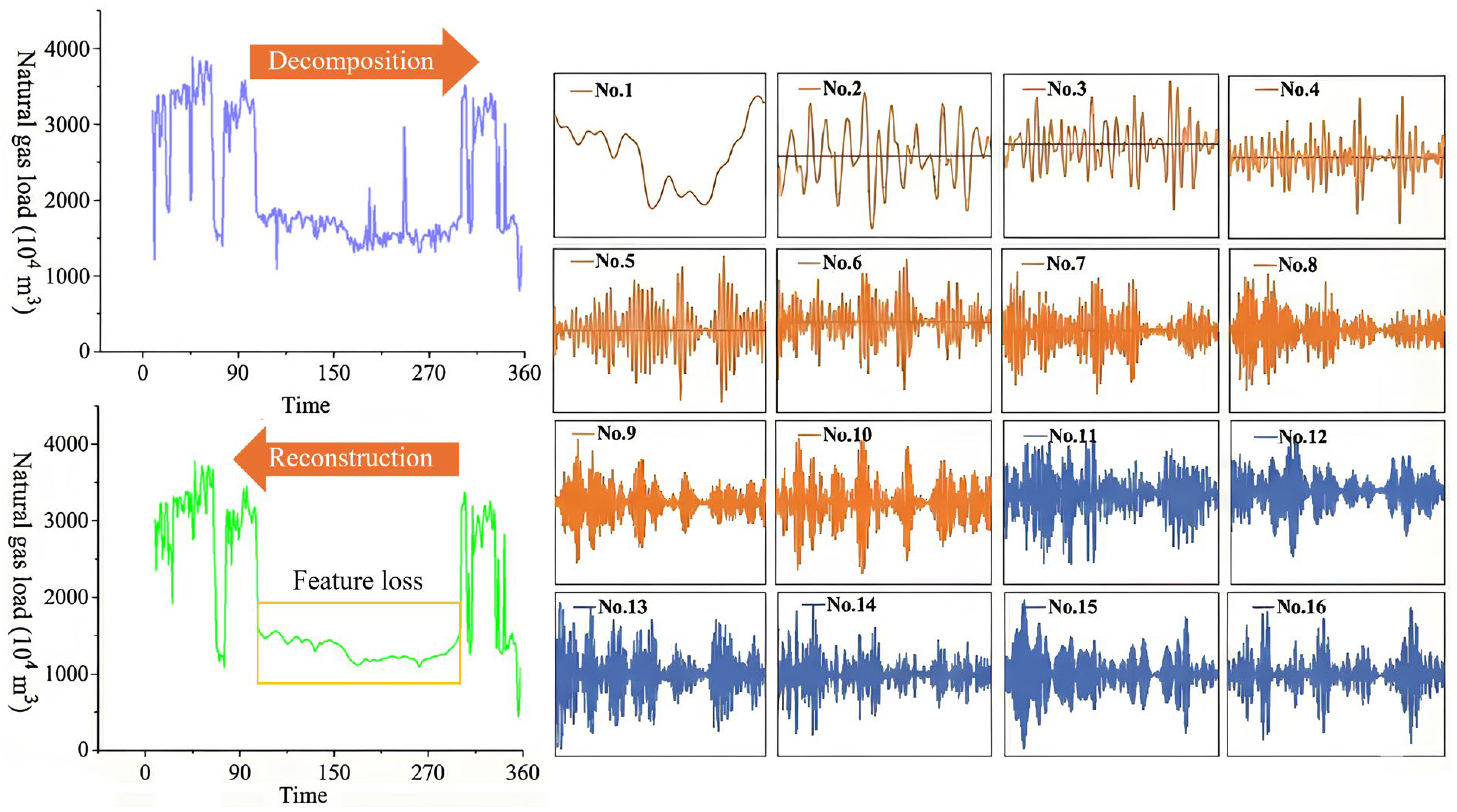
Figure 3 illustrates the denoising results of applying the original SSA algorithm to the same natural gas load data from the large city in Northern China (as used in subsequent experiments). The results clearly demonstrate a significant problem of data feature loss.

Based on these results, it is evident that the standard SSA algorithm, during time series reconstruction, selects sub-sequences solely based on their corresponding eigenvalues while disregarding the intrinsic characteristics of the sub-sequences themselves. This leads to unsatisfactory denoising performance, particularly when a large amount of noise is present [60,61]. When the SSA threshold is set too low, the resulting fitted curve is overly smooth, leading to low fidelity (underfitting); conversely, when the threshold is set too high, the curve fits the data closely but is prone to overfitting [51,52].

2.2.2. Introducing Skewness Logarithm and Kurtosis Logarithm into SSA

To enhance the denoising capability of the Singular Spectrum Analysis (SSA) algorithm for natural gas load data characterized by non-Gaussian distributions and high-skewness “spikes,” and to prevent the occurrence of overfitting or underfitting, this study proposes the Improved Singular Spectrum Analysis (ISSA) algorithm. Building upon the original algorithmic structure, ISSA introduces log-skewness and log-kurtosis to modify the selection process of the standard SSA. The structural framework of ISSA remains identical to that of SSA; the distinction lies in the selection methodology. Specifically, a log-skewness function, s, and a log-kurtosis function, k, are established to measure the probability distribution of the subsequences. The objective is to identify and eliminate high-frequency subsequences that contain significant noise components. The detailed process is described in Equations (4) through (7):

$$s_p=\lg (\left|Skew(Z_p)\right|)=\lg (\left|E\left[{({\displaystyle \frac{Z_p-{\mu }_p}{{\sigma }_p}})}^4\right]\right|)$$

(4)

$$k_p=\lg (\left|Kurt(Z_p)-3\right|)=\lg (\left|E\left[{({\displaystyle \frac{Z_p-{\mu }_p}{{\sigma }_p}})}^4\right]-3\right|)$$

(5)

$$Y_p=\left\{\begin{array}{l}{Z}_p,if{\mathrm{s}}_p\ge {\mathrm{s}}_{t}or{\mathrm{k}}_p\ge k_t,1\le p\le d\\ 0,otherwise,1\le p\le d\end{array}\right.$$

(6)

$$Y={\displaystyle \sum _{p=1}^d{Y}_p}$$

(7)

where s_p is the logarithmic skewness of the sub-series Z_p; k_p is the logarithmic kurtosis of the sub-series Z_p; Skew(Z_p) is the skewness coefficient of the sub-series Z_p; Kurt(Z_p) is the kurtosis coefficient of the sub-series Z_p; μ_p is the mean of the sub-series Z_p; σ_p is the variance of the sub-series Z_p; s_t is the skewness threshold; k_t is the kurtosis threshold; Y is the reconstructed time series.

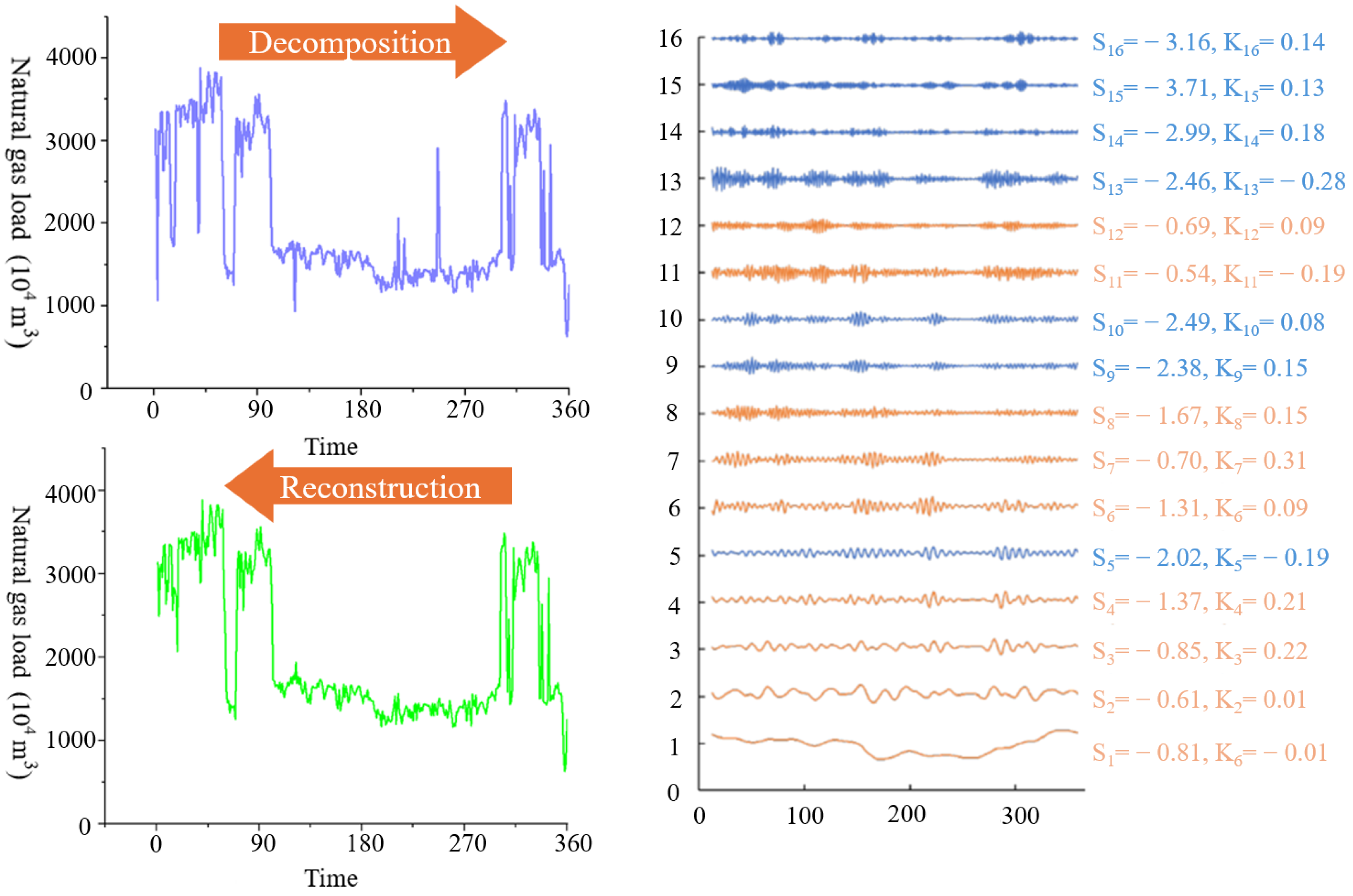
As illustrated in Figure 4, the original data is first decomposed into one low-frequency sub-series and several high-frequency sub-series. Then, the logarithmic skewness s and logarithmic kurtosis k are calculated for each sub-series, and the results are compared against the predefined thresholds s_t and k_t. The rationale is that the smaller the values of s_p and k_p, the more closely the sub-series Z_p approximates a Gaussian distribution. When these values fall below their respective thresholds, the component is identified as noise and is discarded from the dataset. Finally, the sub-series with s and k values greater than the given thresholds are summed to form the reconstructed time series.

As seen visually in the results from Figure 4, the improved ISSA algorithm achieves a significantly better denoising effect on the experimental data. It also markedly remedies the problem of data feature loss, as the key oscillation characteristics of the natural gas load in the central region are fully preserved.

2.3. GRU Neural Network

The Gated Recurrent Unit (GRU) neural network is characterized by its fast convergence speed and simple structure [62]. As shown in Figure 5, the hidden state h represents the degree to which the hidden state from the previous time step is combined with the candidate hidden state of the current time step, a process controlled by the update gate. The candidate hidden state $\tilde{h}$ represents whether the information from the previous time step’s hidden state (which contains historical time series information) is needed for the current time step’s candidate hidden state, as controlled by the reset gate.

The output of the GRU, the calculation formula for y_t is $y_t=\sigma (W_o·h_t)$. The parameters to be learned are the weight matrices W, Wr, Wz and Wo. The relationship between these weights is shown in Equation (8):

$$\begin{array}{l}{W}_r=W_{rx}+W_{rh}\\ W_z=W_{zx}+W_{zh}\\ W=W_{\tilde{h}x}+W_{\tilde{h}h}\end{array}$$

(8)

The specific training steps for these weight parameters are as follows:

(1)

Calculate the input to the output layer ${y_t}^i=W_{o}h$, and the final output $y_t^o=\sigma (y_t^i)$.

(2)

Define the loss function at time step t as $E_t={(y_d-y_t^o)}^2/2$. The total loss for a single sample is then given by $E={\sum }_{t=1}^T{E}_t$.

(3)

Compute the partial derivatives of the total loss function.

(4)

Calculate the relevant weight gradients to update Wr, Wz, W and Wo.

2.4. Construction of the PCCA-ISSA-GRU Model

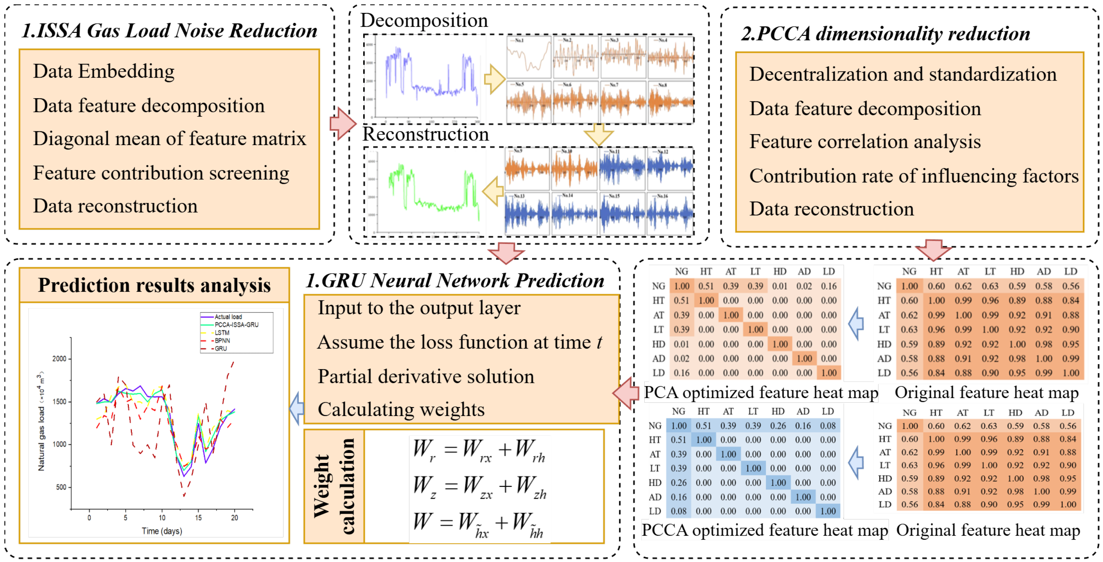
By integrating the improved dimensionality reduction and denoising methods with the GRU network, we establish a novel hybrid model for short-term gas load forecasting, named the PCCA-ISSA-GRU model. The specific workflow of this model is illustrated in Figure 6.

This model framework processes the data from two distinct perspectives: denoising the load data and reducing the dimensionality of the influencing factors. This comprehensive preprocessing aims to achieve higher forecasting accuracy. Specifically, the ISSA algorithm is applied to denoise the historical gas load data. Concurrently, the PCCA algorithm is used to perform a Pearson correlation analysis and extract the key features from the influencing factors after dimensionality reduction. Finally, the denoised and dimension-reduced data are fed into the GRU model to ensure the precision of the gas load forecast.

To ensure model reproducibility and strictly avoid “Data Leakage,” all experiments in this study adhere to a rigorous data partitioning and preprocessing workflow. Data leakage refers to the unintentional use of information from the test set during model training, a common pitfall in time series decomposition or normalization.

The PCCA-ISSA-GRU network processing workflow ensures that information from the test set remains “unseen” until model training is complete:

(1)

Data Splitting: First, the entire dataset is strictly divided into a training set and a test set. For example, in the 20-day prediction experiment, the dataset is split into the first 345 days (training set) and the subsequent 20 days (test set).

(2)

Fit: The parameters of the preprocessing algorithms are fitted only on the training set. Specifically,* The transformation matrix and correlation contribution rates for the PCCA algorithm are calculated based only on the 345-day training data.* The statistical thresholds (S_t and K_t) used by the ISSA algorithm for denoising are determined by analyzing only the historical load series of the 345-day training set.

(3)

Transform: Using the parameters fixed in step (2) (i.e., the PCCA transformation matrix and ISSA thresholds), the transformation is applied separately to both the training set and the test set.

(4)

Model Training: Finally, the preprocessed training set data is fed into the GRU network for training. The trained model is then used to predict the test set, which has undergone the same transformation as in step (3). This “Train-Fit, Test-Transform” workflow [45] ensures the fairness of the forecasting process and the validity of the results.

To ensure the transparency and reproducibility of the experiment,

Table 2. Key Hyperparameters for the PCCA-ISSA-GRU Model and Baseline Models.

Model	Parameter	Setting/Range	Search Space/Candidate Set	Selection Basis
PCCA	SP	90%	{80%, 85%, 90%, 95%, 99%}	Sensitivity Analysis
ISSA	St	0.5	{0.1, 0.3, 0.5, 0.7, 0.9}	Sensitivity Analysis
PCCA-ISSA-GRU	Hidden units	64	{32, 64, 128, 256}	Grid Search (Minimizing Validation Loss)
	Layers	2	{1, 2, 3}	Trial and Error
	Optimizer	Adam	{Adam, SGD, RMSprop}	Standard Algorithm
	Learning rate	0.001	[0.0001, 0.01]	Grid Search
	Batch size	32	{16, 32, 64, 128}	Trade-off between speed and stability
	Loss function	MSE	{MSE, MAE, RSE, RAE}	Standard Regression Metric
GRU	Hidden units	64	-	Consistent with Proposed Model (Fairness)
LSTM	Hidden units	64	-	Consistent with Proposed Model (Fairness)
BPNN	Hidden layers/units	[10, 10]	{[10], [10, 10], [20, 10]}	Empirical Tuning
ARIMA-ANN	Order (p, d, q)	(1, 1, 1)	Grid Search based on AIC	Akaike Information Criterion (AIC)
Informer (SOTA)	Encoder layers	2	{1, 2, 3, 4}	Standard Setting
	Decoder layers	1	{1, 2}	Standard Setting
	Attention heads	8	{4, 8, 16}	Default Configuration
	FFN dimension	2048	{1024, 2048}	Default Configuration
	Activation function	GeLU	{ReLU, GeLU}	Standard for Transformers

Note: The Adam optimizer follows the standard implementation by Kingma & Ba (2014) [63]. The Informer model parameters follow the original configuration by Zhou et al. (2021) [53].

details the key hyperparameters for the PCCA-ISSA-GRU model and the baseline models. Parameters for other baseline models were obtained using recommended values from the literature, combined with fine-tuning.

3. Load Characteristics and Influencing Factor Analysis

3.1. Load Feature Analysis

To validate the accuracy of the novel hybrid algorithm in short-term natural gas load forecasting (NGLF), this study conducts an empirical analysis based on actual gas load data from a large city in Northern China (using the same data as in the PCA and SSA algorithm improvement sections). Accurate load forecasting is the core link in ensuring the reliability of gas supply, optimizing pipeline network planning, and managing daily dispatch. It provides critical technical support for the decision-making of urban gas management departments.

The gas load data for this city exhibits complex, composite characteristics:

(1)

First: due to the regular patterns of social production and residential life, the load demonstrates significant periodicity on daily, weekly, and annual scales.

(2)

Second: in the absence of special events, the data changes smoothly, showing continuity.

At the same time, the presence of numerous users with diverse consumption habits, coupled with interference from various external factors such as weather and holidays, imparts strong randomicity and non-linearity to the load fluctuations, which poses a significant challenge for precise forecasting.

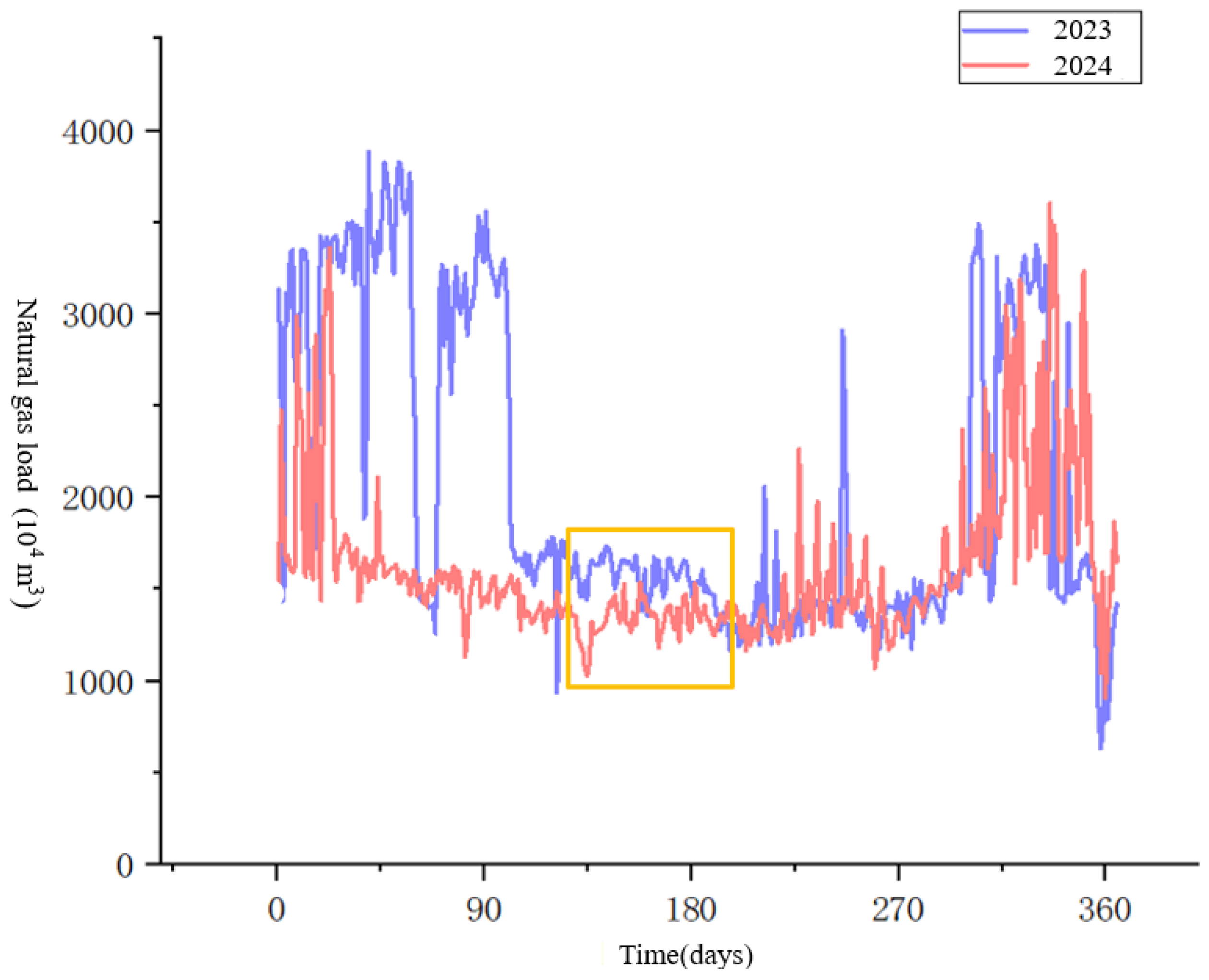
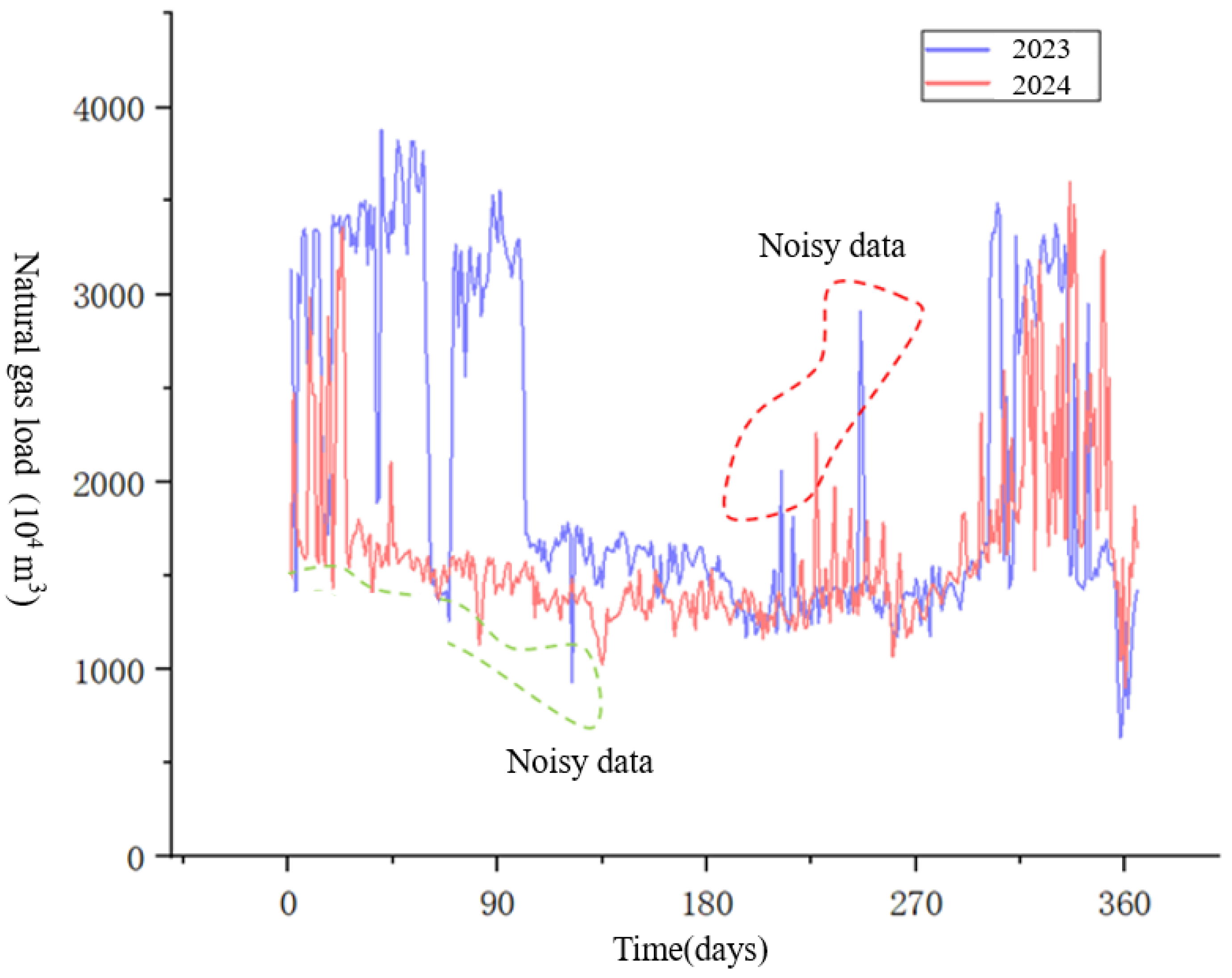
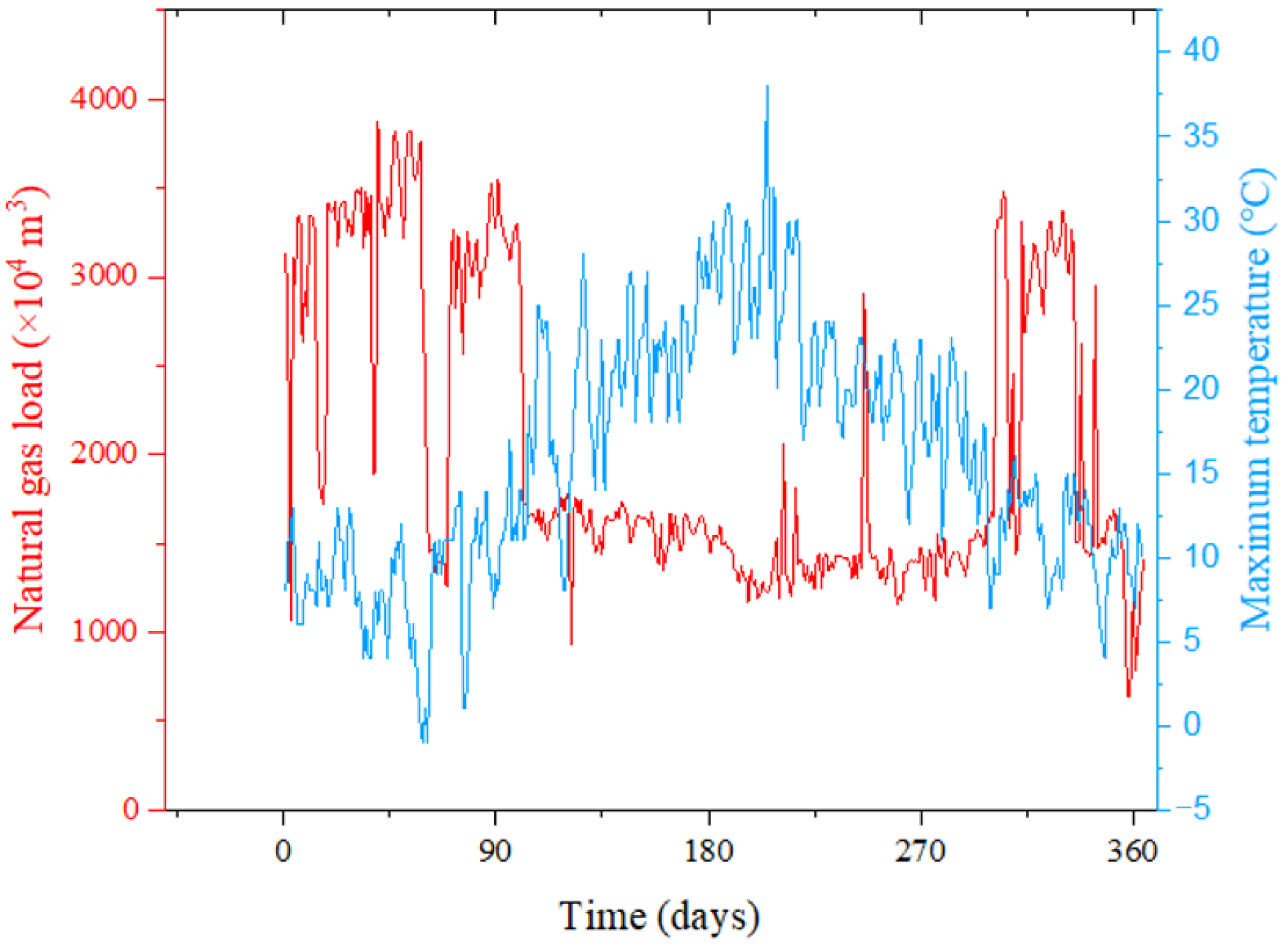
From a macroscopic trend perspective, the city’s daily load data presents a distinct seasonal pattern of being “high in winter and low in summer,” but it is also characterized by intense short-term volatility and data anomalies. As shown in Figure 7, the load curves for 2023 and 2024 intuitively verify this set of complex characteristics.

Noisy data, also known as outlier data in natural gas load forecasting (although the two are often distinct), refers to data that deviates from the true value due to factors such as metering instrument errors, operator recording errors, and statistical errors. Typically, it mainly refers to the high-frequency components in the raw data. The deviation of noisy data from the true value is difficult to identify by directly observing the load trend curve. Load data contains many outliers that differ significantly from the true value. As shown in Figure 8, the presence of these outliers severely affects prediction accuracy and reduces the performance of the prediction model. Therefore, how to handle outlier data is a primary issue to be addressed in short-term natural gas load forecasting. Improper handling will affect the training effect of the prediction model and increase the difficulty of prediction. Numerous studies have shown that using data denoising algorithms to reduce noise in the raw data can effectively improve prediction accuracy and reduce short-term load forecasting errors.

Thus, to obtain higher prediction accuracy, it is necessary to adopt effective denoising methods to mitigate the adverse effects of noise on NGLF. The improved ISSA algorithm can accurately identify data noise while preserving the original data characteristics, providing a reliable data source for subsequent prediction (the denoising results using ISSA are shown in Section 2.2).

3.2. Analysis of Influencing Factors

In short-term natural gas load forecasting (NGLF), it is necessary to analyze a large number of continuous daily load-influencing factors. Therefore, when considering these factors, one must account for not only their correlation with the gas load but also their feasibility (i.e., data availability and reliability for a predictive context). Based on these considerations, the primary factors ultimately identified for daily NGLF include weather conditions, date types, wind levels, and holiday factors. After analyzing the relevant factors using the improved PCCA algorithm, the following two key factor groups were identified (a detailed correlation analysis is provided in Section 2.1):

(1)

Meteorological Factors

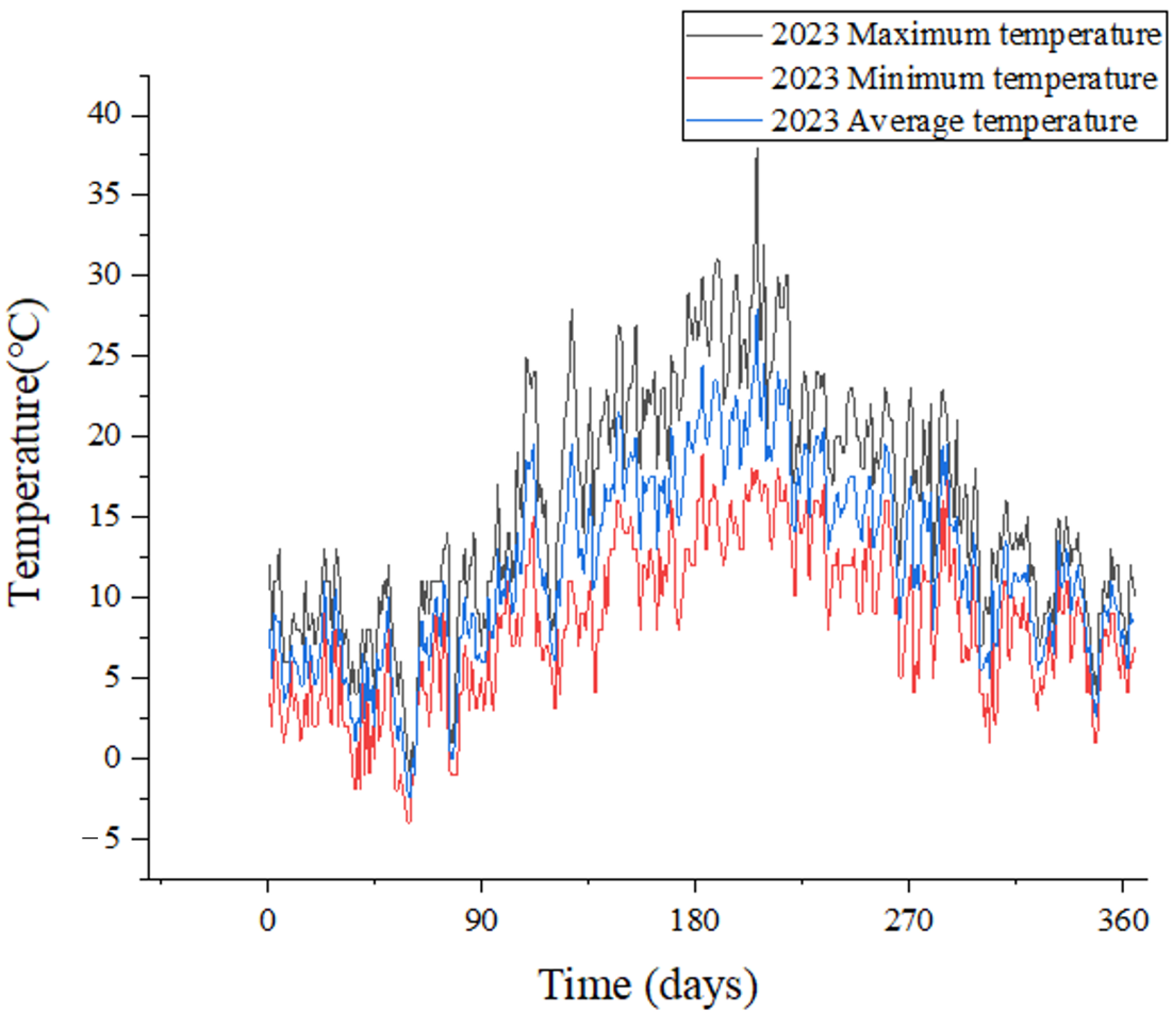
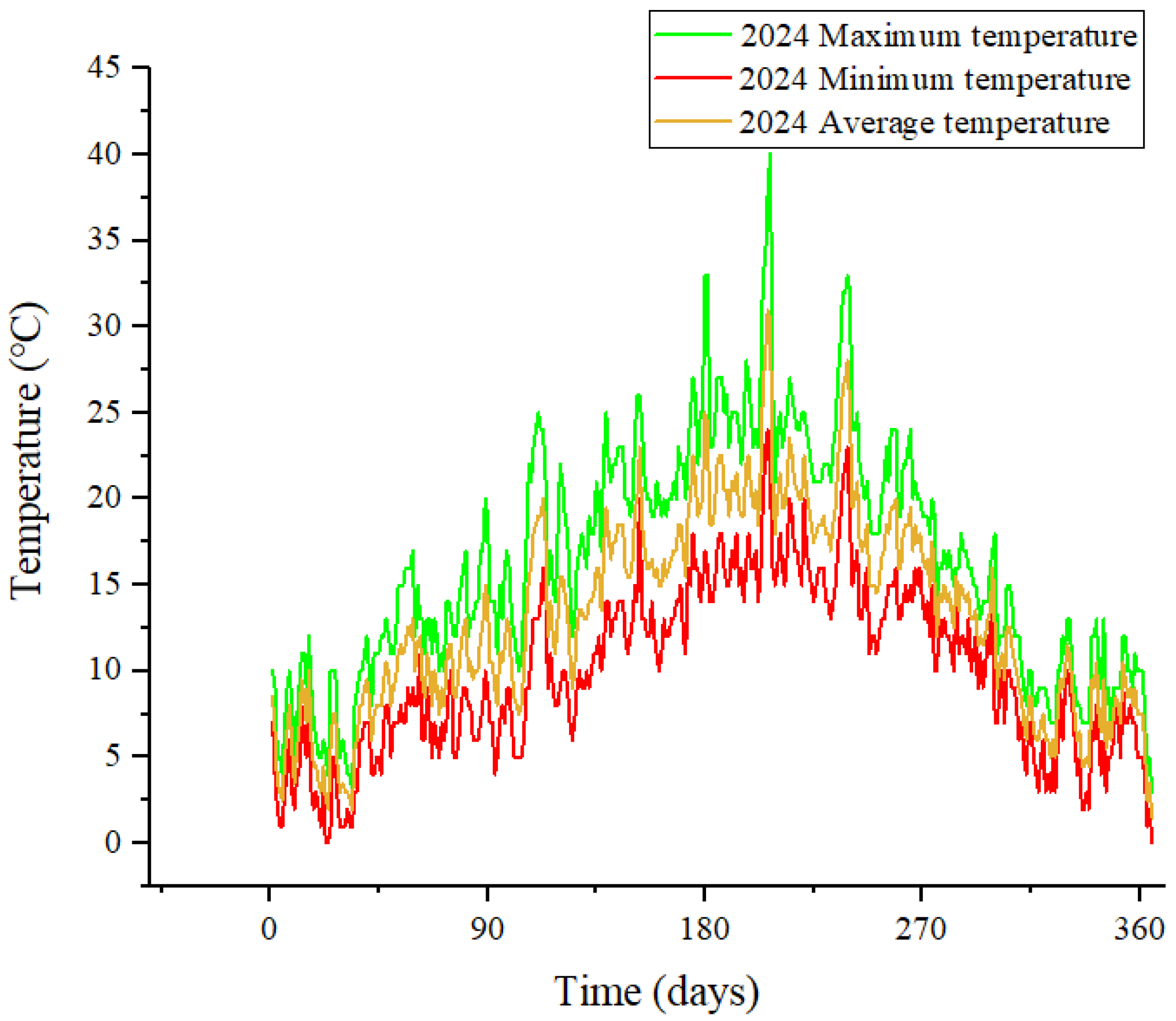
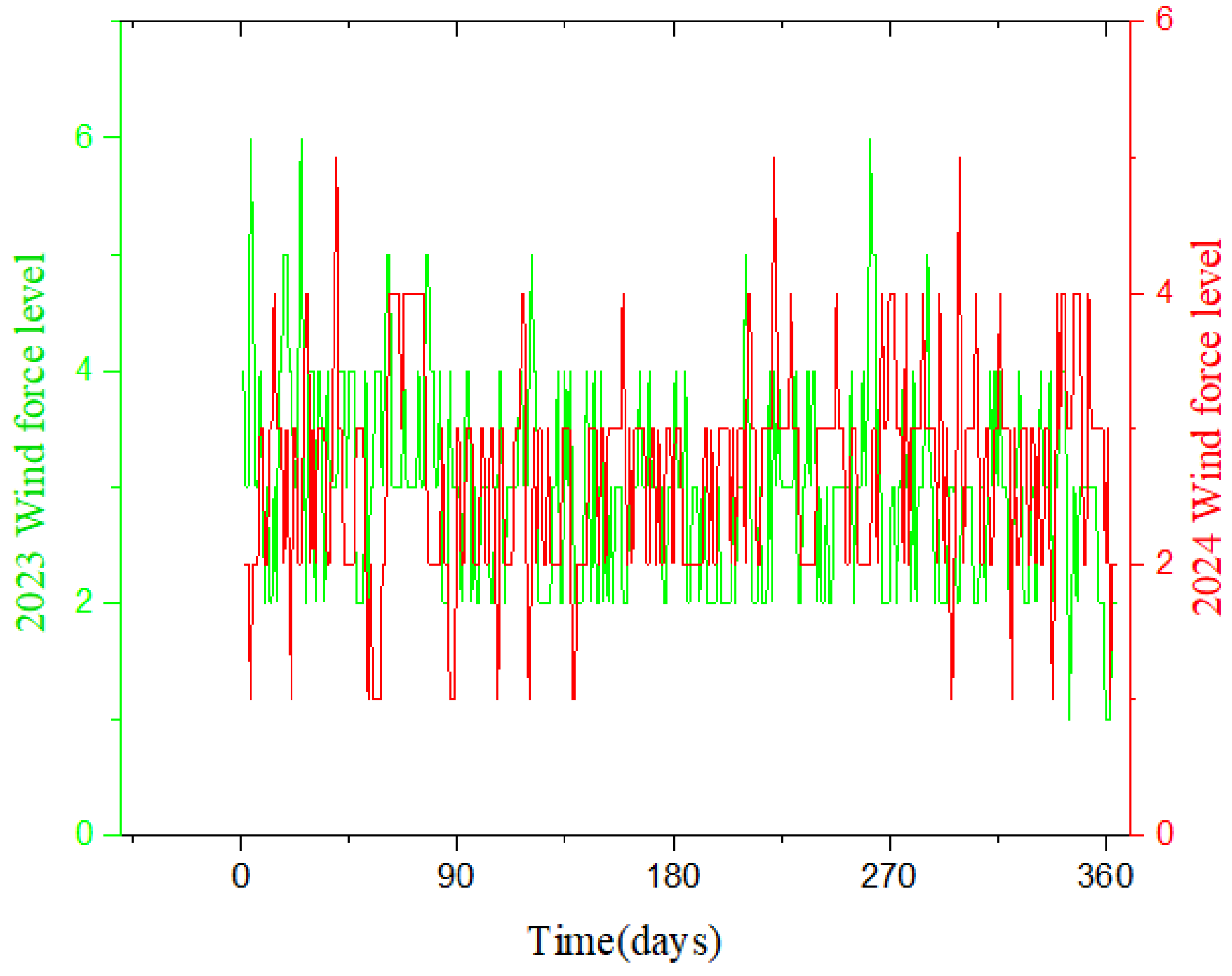
The analysis from the improved PCCA algorithm confirms that meteorological factors are the primary drivers influencing the natural gas load in the studied city. In different seasons, gas consumption is inextricably linked to changes in factors such as temperature and wind level. Consequently, meteorological factors are the foremost choice for short-term NGLF. Specific factors include daily maximum temperature, daily minimum temperature, daily average temperature, and wind level. This paper collected and organized relevant temperature and wind data for a specific city in China for the years 2023 and 2024, as shown in Figure 9, Figure 10 and Figure 11.

Among these, the maximum temperature is the single most significant factor influencing the load variation in this city. Figure 12 illustrates the correlation between load and maximum temperature. The horizontal and vertical axes represent time, temperature, and gas load value, respectively. As can be observed from the figure, the lower the temperature, the higher the gas load. As the temperature rises, the load value decreases, demonstrating a clear negative correlation between temperature and load.

(2)

Date and Price Factors

Date factors include the year, month, and day. These factors not only convey date information but also indirectly reflect holiday information, which is correlated with user gas consumption patterns. For example, during public holidays, many people choose to travel, leading to a significant drop in gas consumption, whereas consumption on weekdays remains relatively stable.

Regarding price factors, it was determined that gas price should not be used as an input variable for short-term NGLF. This decision is based on two facts: first, in the short term, the price of natural gas generally does not undergo drastic changes. Second, the gas price for a future (forecasted) period is often unknown. If a predicted gas price were used as an input variable to forecast the future gas load, the uncertainty inherent in the price prediction could itself lead to deviations in the final load forecast. Therefore, gas price is excluded as an input variable for the short-term model.

4. Results and Discussion

4.1. Parameter Sensitivity Analysis

To ensure model reproducibility, a sensitivity analysis was conducted on the most critical hyperparameters of the PCCA-ISSA-GRU model: (1) the number of GRU hidden units; and (2) the PCCA cumulative contribution threshold (S_P) and the ISSA skewness threshold (S_t).

Based on the experimental data samples, the analysis was performed under a 20-day forecast horizon. The impact of the number of GRU hidden units on MAPE was evaluated using a controlled variable approach, where one parameter was varied while others remained constant. The results are presented in

Table 3. PCCA-ISSA-GRU Key Hyperparameter Sensitivity Analysis (20-day forecast).

Parameter	Test Value	MAPE (%)
GRU Hidden Units	32	6.25
	64	6.09
	128	6.18
	256	6.75

.

As shown in Table 3, different numbers of hidden units were tested in the hyperparameter tuning experiments to evaluate their impact on prediction performance. The results indicate that the model achieved optimal performance with 64 hidden units, yielding the lowest MAPE of 6.09%. Insufficient units may lead to underfitting, whereas excessive units tend to induce overfitting.

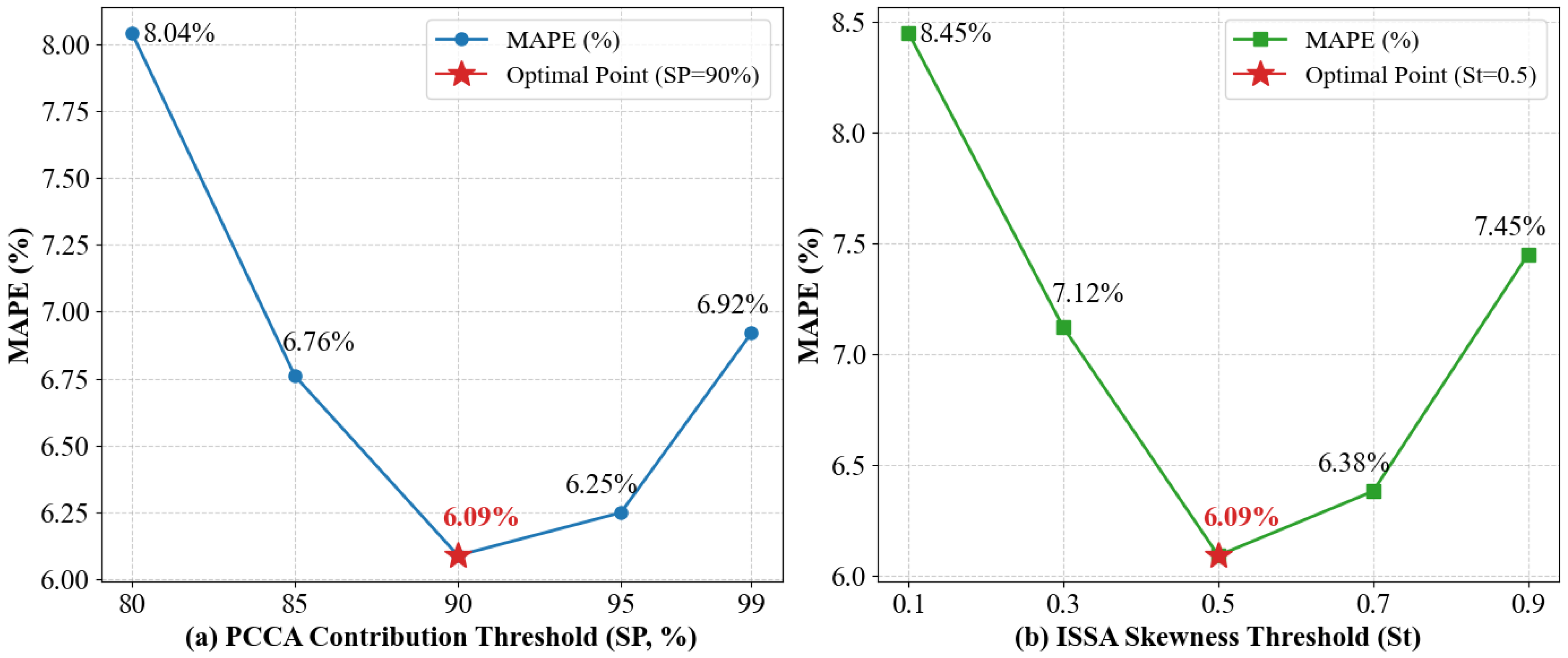
In the PCCA-ISSA-GRU model, the PCCA cumulative contribution rate threshold (S_P) and the ISSA skewness threshold (S_t) are crucial hyperparameters determining feature quality and signal purity. To validate the rationale of the selected parameters (S_P = 90, S_t = 0.5) and investigate the impact of parameter variations on prediction performance, a dual-parameter sensitivity analysis was conducted. Using the controlled variable approach, the model’s MAPE was tested under different parameter configurations, as illustrated in Figure 13.

As shown in Figure 13a, the selection of the PCCA threshold S_P requires a trade-off between “information integrity” and “feature redundancy”:

(1)

Underfitting Region (S_P < 90%): When S_P is low (e.g., 80%), the model discards critical features that are non-linearly correlated with the load, resulting in a high MAPE (8.04%).

(2)

Overfitting Region (S_P > 90%): When S_P is excessively high (e.g., 99%), the model incorporates numerous tail features containing noise. This increases computational complexity and interferes with prediction, causing the error to rise to 6.92%.

(3)

Optimal Point (S_P = 90%): At this level, the model retains the vast majority of valid information while eliminating redundancy, achieving the lowest error (6.09%).

As shown in Figure 13b, the ISSA threshold S_t determines the “intensity” of signal denoising, exhibiting a similar “decrease-then-increase” trend:

(1)

Over-smoothing (S_t < 0.5): When the threshold is set too low (e.g., 0.1), the screening criteria of the ISSA algorithm become overly strict. Consequently, many normal high-frequency signals containing sudden load changes are erroneously identified as noise and removed. This “over-cleaning” destroys the authentic structure of the raw data, keeping MAPE at a high level (8.45%).

(2)

Residual Noise (S_t > 0.5): When the threshold is set too high (e.g., 0.9), the screening criteria become too lenient. The algorithm fails to effectively identify non-Gaussian random noise, allowing significant interference signals to remain in the input sequence. This reduces the learning efficiency of the GRU, causing MAPE to rise to 7.45%.

(3)

Optimal Balance (S_t = 0.5): When S_t is set to 0.5, the model accurately distinguishes between valid high-frequency fluctuations and random noise, maximizing the restoration of the true load variation patterns and achieving optimal prediction accuracy.

The results indicate that the model’s performance remains relatively stable within the ranges of 64 to 128 for GRU hidden units, 90% to 95% for the PCCA threshold, and 0.5 to 0.7 for the ISSA threshold. This demonstrates that the PCCA-ISSA-GRU framework possesses excellent robustness and does not rely on extreme “fine-tuning” of hyperparameters.

4.2. Comparative Analysis with Classic Single Models

To comprehensively validate the effectiveness of the proposed framework, this section selects three representative types of standalone models as baselines: BPNN, LSTM, and GRU. The rationale for selecting these models is as follows:

(1)

Foundational ANN Baseline: The Back-Propagation Neural Network (BPNN) was chosen as the most fundamental neural network model. Its simple structure represents an early application of neural networks in the forecasting domain. Comparing against it serves to establish a performance “low-bar” baseline, used to measure the necessity of more complex models designed for time-series data.

(2)

“Gold-Standard” Sequential Baselines: Long Short-Term Memory (LSTM) and Gated Recurrent Unit (GRU) are the current “gold standard” and established best practices in the field of time-series forecasting. Both models are specifically designed to capture long-term temporal dependencies in data via sophisticated gating mechanisms, which is crucial for load forecasting. Comparing PCCA-ISSA-GRU against these two classic recurrent neural networks is a necessary step to evaluate whether its performance reaches the state-of-the-art (SOTA) level in the domain.

(3)

“Ablation” Validation of Core Components: Critically, the core of the model proposed in this study is the GRU. Therefore, comparing the PCCA-ISSA-GRU (i.e., “PCCA feature selection + ISSA data cleansing + GRU prediction”) with an original, unprocessed GRU model constitutes a key part of an ablation study. The purpose of this comparison is to clearly isolate and quantify the actual performance improvement brought about by our innovative PCCA-ISSA preprocessing framework, rather than attributing the success solely to the GRU architecture itself. This directly validates the effectiveness and contribution of this study’s primary innovation (the front-end preprocessing).

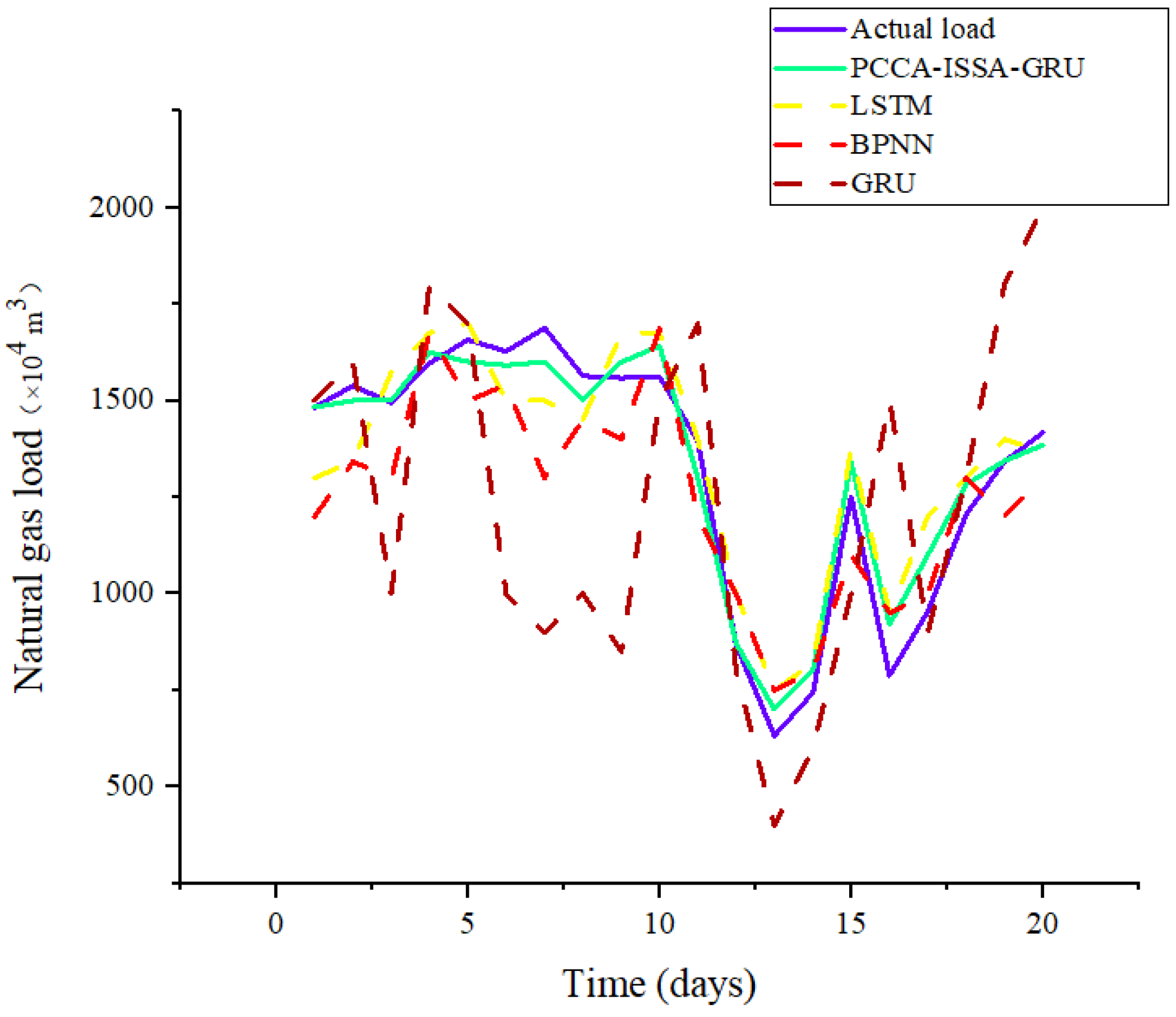
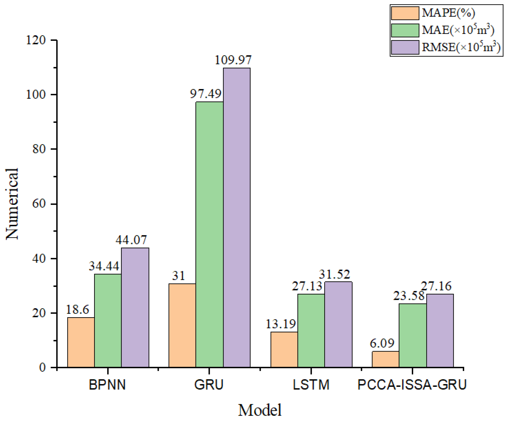
After analyzing the load data, the experiment was set with a forecast horizon of 20 days. The hybrid algorithm (PCCA-ISSA-GRU) applied the improved PCCA algorithm for dimensionality reduction in influencing factors and the improved ISSA algorithm for data cleansing to forecast the load data. A comparative analysis was conducted against the prediction results of the LSTM, BPNN, and GRU models. The comparison results are shown in Figure 14 and Figure 15.

As indicated by the prediction results, in the short-term forecasting scenario, the prediction accuracy of the PCCA-ISSA-GRU hybrid model is significantly higher than that of the traditional models, exhibiting the lowest MAPE, MAE, and RMSE.

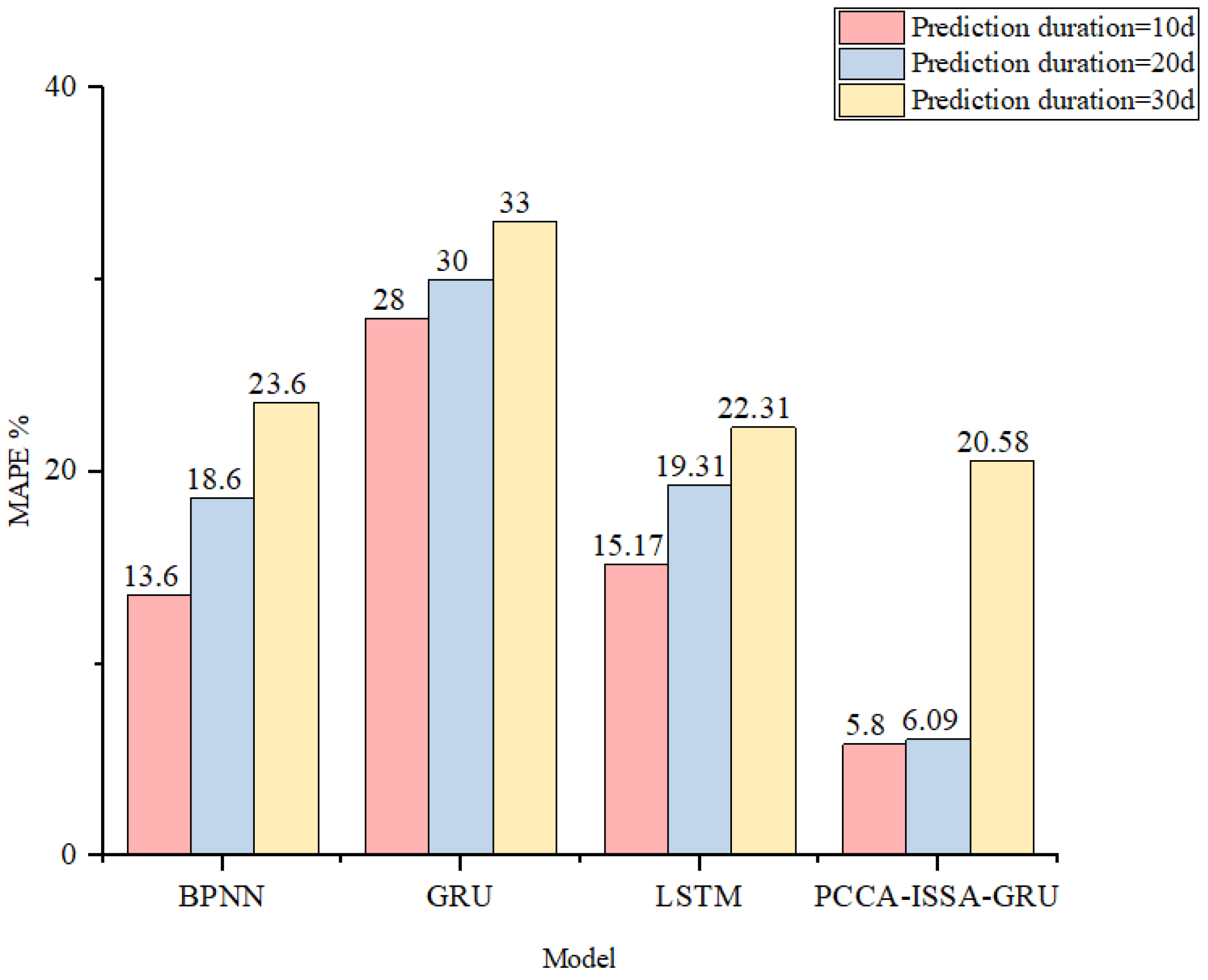
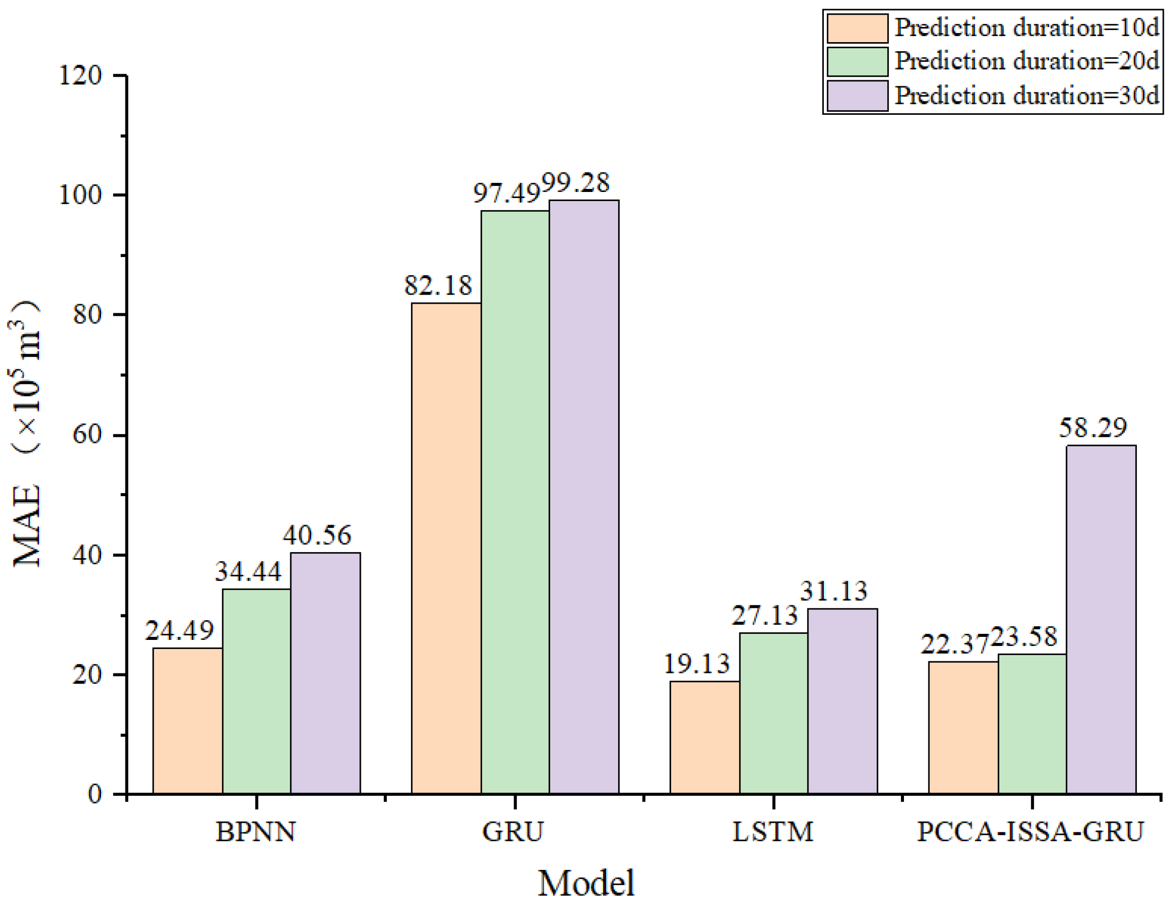
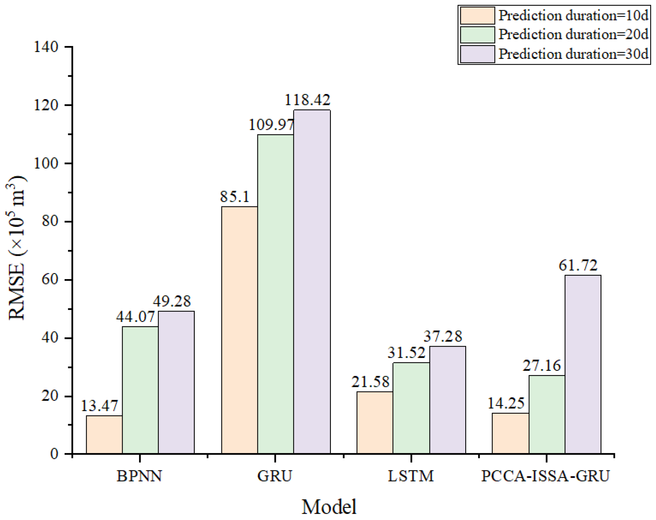
On this basis, to further verify the adaptability of the hybrid model for short-term NGLF, this paper designed three experimental groups using the PCCA-ISSA-GRU model, based on different forecast horizons. Each group has a training and test set of varying lengths, as shown in

Table 4. Summary of Different Prediction Durations.

Prediction Duration	Training Set (Data Volume)	Test Set (Data Volume)
10	1 January 2024–21 December 2024 (356)	22–31 December 2024 (10)
20	1 January 2024–11 December 2024 (346)	12–31 December 2024 (20)
30	1 January 2024–1 December 2024 (336)	2–31 December 2024 (30)

. The error results for the four models are shown in Figure 16, Figure 17 and Figure 18.

As can be seen from Figure 16, Figure 17 and Figure 18, when the forecast horizon is 20 days, the three error metrics for the hybrid forecasting model are likewise lower than those of the other three existing models. Furthermore, the same trend holds: the shorter the prediction horizon, the higher the accuracy.

Additionally, when extending the forecast horizon from 20 days to 30 days, the MAPE value for the PCCA-ISSA-GRU hybrid model triples (a 3-fold increase) compared to its 20-day MAPE. In contrast, the MAPE increases for the BPNN, GRU, and LSTM models were 26.88%, 10.00%, and 15.54%, respectively. The results show that all three baseline models and the PCCA-ISSA-GRU hybrid model experience a surge in error. This is related to the construction of the neural networks; whether it is the BP error back-propagation mechanism or the LSTM/GRU long-term memory mechanism, the iterative (step-by-step) forecasting process inevitably leads to error accumulation, causing the prediction results to gradually deviate from the true values. Therefore, the proposed hybrid model is more suitable for short-term load forecasting analysis within a 20-day horizon.

After the PCCA feature selection, the daily maximum temperature was selected as the characteristic variable for the predictive model, rather than the daily average temperature. To verify the accuracy of this selection, three sets of experiments were conducted using the daily average temperature as the characteristic variable, while all other feature variables remained unchanged.

Table 5. Model Errors for Different Temperature Types.

Model Type	Temperature Type	Prediction Duration (Days)	MAPE (%)	MAE (105 m3)	RMSE (105 m3)
PCCA-ISSA-GRU	Maximum temperature	10	5.80	22.30	14.25
		20	6.09	23.58	27.16
		30	20.58	58.29	61.71
PCCA-ISSA-GRU	Average temperature	10	10.47	37.71	43.15
		20	11.65	39.47	37.45
		30	27.45	70.14	88.54

displays the error values of the prediction results.

It is evident from Table 5 that for this particular city, the correlation between maximum temperature and users’ natural gas consumption is stronger than that between average temperature and consumption. This indicates that when applying this hybrid forecasting model, the maximum temperature should be considered a key factor. These experimental results indirectly validate the accuracy of the PCCA method for selecting the features of influencing factors.

4.3. Comparison with Classic Hybrid Algorithms and SOTA Algorithms

To further situate the PCCA-ISSA-GRU model within a broader academic context, this section introduces two more advanced predictive models for comparison: ARIMA-ANN and Informer. The rationale for their selection is as follows:

(1)

Classic Hybrid Model Baseline: The ARIMA-ANN model was selected as a representative of “classic hybrid forecasting models.” Before deep learning (especially Transformer) architectures became dominant, hybrid paradigms combining statistical models like ARIMA with ANNs were a powerful and widely adopted technique for handling complex time-series forecasting (addressing both linear and non-linear components). The comparison against ARIMA-ANN aims to demonstrate that the framework proposed in this study holds a performance advantage over these mature hybrid forecasting paradigms.

(2)

State-of-the-Art (SOTA) Baseline: The Informer model was selected as the SOTA baseline. As a highly academically influential Transformer-based architecture designed specifically for Long-Series Time-series Forecasting (LSTF), the Informer represents the cutting-edge technology in this field. A benchmark against a SOTA model is necessary to answer two key questions: (a) In terms of prediction accuracy, can the model proposed in this study compete with (or “be comparable to”) the most advanced and structurally complex architectures, such as the Informer? (b) Within the specific medium-to-short-term “tactical planning window” (e.g., 10–20 days), can this study’s “advanced domain-specific preprocessing + lightweight model” strategy prove to be a more cost-effective and practical solution than a complex SOTA model?

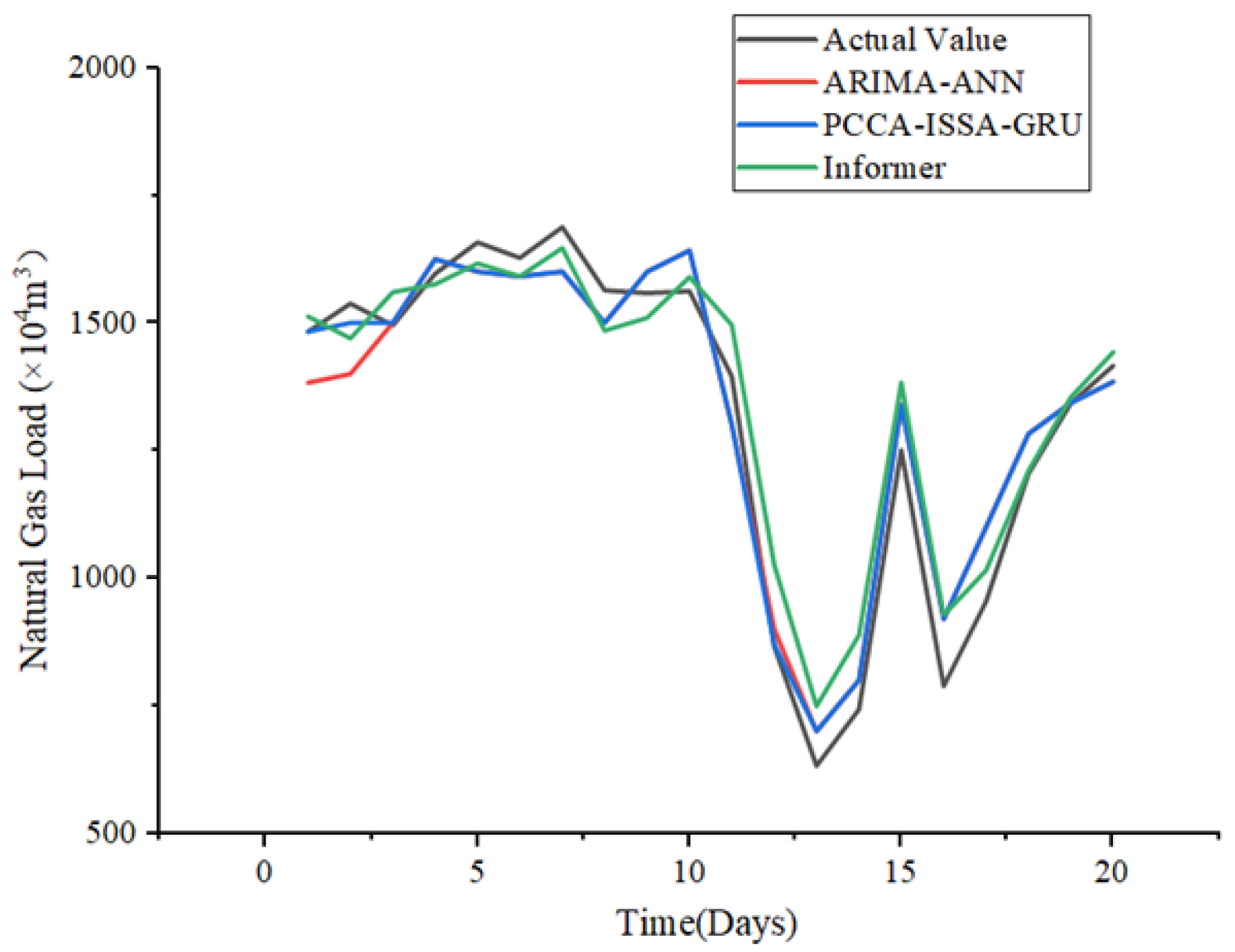
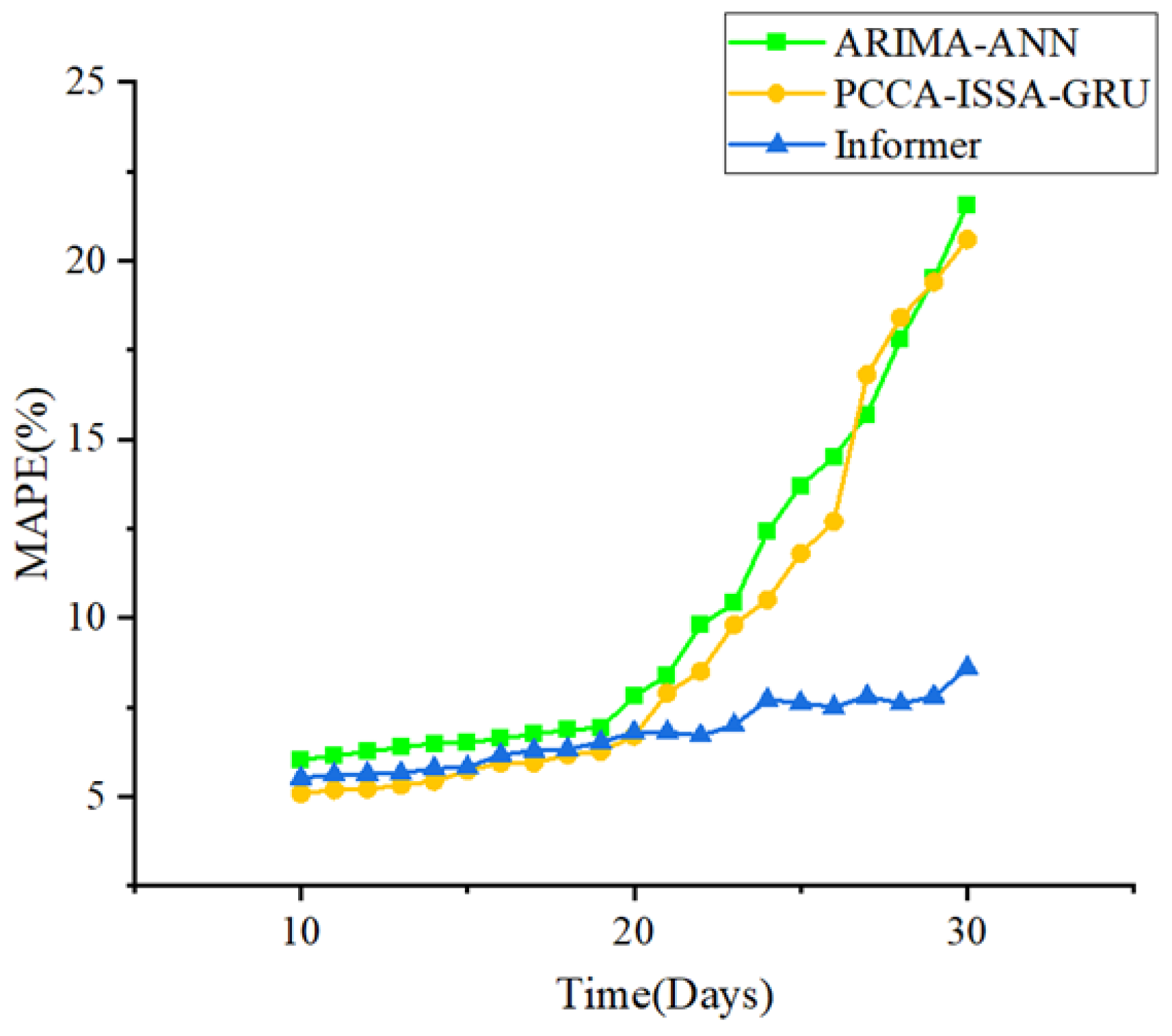
Taking the period from 12–31 December 2024, as an example, the predictive comparison results are shown in Figure 19, and the MAPE values are shown in Figure 20.

Through the comparative analysis of Figure 18 and Figure 19, it can be concluded that the classic ARIMA-ANN hybrid model exhibits some volatility in the initial forecasting stage. The novel PCCA-ISSA-GRU hybrid forecasting model’s results are more stable, whereas the Informer model shows an advantage in the later forecasting stage. Overall, the PCCA-ISSA-GRU hybrid model achieves ideal prediction results in both the early and late stages.

An analysis of the MAPE results reveals that the new hybrid model is more suitable for urban NGLF. Within the 10-day and 20-day “tactical planning window,” the MAPE metrics for PCCA-ISSA-GRU (5.80% and 6.09%) are both slightly superior to those of the Informer model (6.25% and 6.51%).

When the forecast horizon exceeds 20 days, the error of the PCCA-ISSA-GRU model increases significantly. This is attributed to the auto-regressive mechanism of its GRU core, which is prone to error accumulation in long-sequence forecasting, leading to a decline in accuracy in the later stages. In contrast, the Informer model, as the SOTA baseline, maintained high stability in its MAPE throughout the entire period. This is because it employs a Transformer-based direct multi-step prediction strategy, which circumvents the problem of error accumulation and demonstrates its architectural advantage in LSTF tasks.

During the comparative experiments, it was found that although the Informer, as a SOTA model, exhibited powerful predictive capabilities, it is a model with a complex structure, numerous hyperparameters, and requires substantial computational resources for training. In contrast, the PCCA-ISSA-GRU framework is based on a more lightweight GRU, and its core advantage lies in the efficient, targeted front-end preprocessing (PCCA and ISSA), rather than a complex model architecture.

For the NGLF “tactical planning window” (10–20 days), PCCA-ISSA-GRU achieves a level of accuracy comparable to or even slightly better than Informer, but it possesses significant advantages in terms of model simplicity, tuning difficulty, and training cost. This proves that the “advanced domain-specific preprocessing + lightweight model” strategy is a more cost-effective and practical solution than complex SOTA models in this specific application scenario.

4.4. Significance Testing and Effectiveness Analysis of Core Modules

To rigorously evaluate whether the predictive advantage of the PCCA-ISSA-GRU model over other benchmark models is statistically significant, we employed the Diebold–Mariano (DM) test. While metrics such as MAPE and MAE only indicate “average performance,” the DM test assesses whether the difference in prediction error sequences between two models is statistically meaningful. The DM test is a standard method in time series forecasting as it correctly handles the serially correlated errors inherent in multi-step forecasting.

Using the Mean Squared Error (MSE) of the 20-day forecast (h = 20) as the loss function, we tested whether PCCA-ISSA-GRU (Model A) is significantly superior to other benchmark models (Model B). The null hypothesis (H₀) of the DM test posits that the two models have equal predictive accuracy. If the p-value is less than 0.05, we reject the null hypothesis and conclude that Model A is significantly superior to Model B.

As shown in

Table 6. Diebold–Mariano (DM) Statistical Significance Test.

Comparison	Loss Function	DM Statistic	p-Value	Conclusion (p < 0.05)
vs. BPNN	MSE	4.31	0.0001	Significantly Superior
vs. GRU	MSE	4.52	<0.0001	Significantly Superior
vs. LSTM	MSE	3.28	0.001	Significantly Superior
vs. ARIMA-ANN	MSE	3.05	0.0023	Significantly Superior
vs. Informer	MSE	2.19	0.0285	Significantly Superior

, the p-values for the comparison between the PCCA-ISSA-GRU model and all traditional benchmarks (BPNN, GRU, LSTM, ARIMA-ANN) are well below 0.01, indicating that its advantage is highly statistically significant. More importantly, in the comparison with the SOTA model Informer, the p-value is 0.0285 (<0.05). This statistically confirms that although the lead of PCCA-ISSA-GRU in terms of MAPE for the 10–20-day forecast is relatively small (see Table 6), this advantage is not accidental but statistically significant.

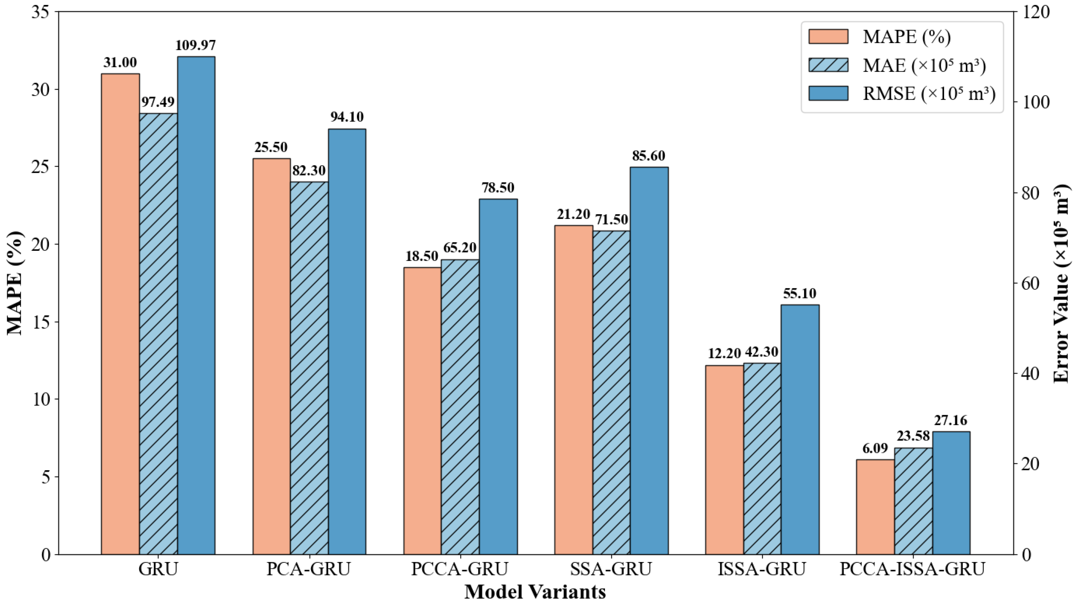
To deeply investigate the specific contributions of the proposed PCCA feature extraction module and the ISSA denoising module to prediction accuracy, and to verify the degree of improvement of PCCA and ISSA algorithms relative to traditional methods, this study conducted an ablation experiment. In addition to the benchmark GRU model, models based on original PCA (PCA-GRU) and original SSA (SSA-GRU) were introduced. Excluding the two unimproved models mentioned above, we used the standard GRU network as a baseline and progressively added innovation modules to construct four comparison models: GRU (baseline), PCCA-GRU (feature optimization only), ISSA-GRU (denoising optimization only), and PCCA-ISSA-GRU (complete hybrid model). The experiment used MAPE, MAE, and RMSE for comprehensive evaluation, and the results are shown in Figure 21.

(1)

PCCA Module Improves Feature Input Quality: Compared with the benchmark GRU model, the PCCA-GRU model showed significant improvement across all metrics. Notably, the Mean Absolute Error (MAE) decreased from 97.49 to 65.20. This indicates that while traditional PCA reduces dimensionality, it often overlooks the correlation between features and the target variable (gas load). By introducing the PCCA algorithm, the model can screen for meteorological factors most sensitive to load changes (e.g., maximum temperature), thereby reducing interference from invalid information at the input stage and enhancing the model’s fitting capability.

(2)

ISSA Module Significantly Reduces Random Fluctuation Interference: The ISSA-GRU model performed even better than PCCA-GRU, with its MAPE dropping to 12.20% and MAE further reducing to 42.30. Urban gas load data contains significant non-Gaussian noise due to sudden events and equipment measurement errors. The ISSA algorithm utilizes skewness and kurtosis metrics to accurately identify and eliminate these high-frequency noise components. Data smoothing enables the GRU network to more easily capture the intrinsic periodic patterns of the load, thereby significantly reducing the absolute bias of the prediction.

(3)

Dual Optimization Achieves Best Performance Superposition: The proposed PCCA-ISSA-GRU model combines the two improvement strategies mentioned above, achieving optimal prediction results. Its MAE ultimately dropped to 23.58, a reduction of approximately 75.8% compared to the benchmark GRU model. This confirms that PCCA and ISSA are not merely a simple stacking of functions but form complementary advantages: ISSA ensures the purity of the Target Data, while PCCA ensures the high correlation of the Explanatory Variables. The synergistic effect of the two maximizes the predictive potential of the deep learning model, fully addressing the limitations of single methods discussed earlier.

(4)

PCCA vs. PCA: Although PCA-GRU (MAPE = 25.50%) showed improvement over the benchmark model, PCCA-GRU (MAPE = 18.50%) performed significantly better. This confirms the limitation of traditional PCA mentioned by reviewers: traditional PCA screens features solely based on variance contribution rates, leading to the loss of critical features (such as specific meteorological factors) that have small variance but high correlation with gas load. PCCA salvages this information through correlation ranking, bringing about an accuracy improvement of approximately 7 percentage points.

(5)

ISSA vs. SSA: Similarly, ISSA-GRU (MAPE = 12.20%) is distinctly superior to SSA-GRU (MAPE = 21.20%). This indicates that when dealing with non-stationary gas load data, traditional SSA often struggles to determine the optimal reconstruction threshold, easily leading to residual noise or over-smoothing. The skewness and kurtosis statistical metrics introduced by ISSA provide an adaptive signal screening mechanism, more effectively separating valid signals from random noise.

To further confirm whether the model is overfitting and to assess its generalization ability,

Table 7. Comparison of training and testing errors to assess model generalization.

Model	Training MAPE (%)	Test MAPE (%)	Generalization Gap	Overfitting Risk
GRU	28.45	31	2.55	Moderate
PCA-GRU	23.1	25.5	2.4	Low
PCCA-GRU	17.8	18.5	0.7	Minimal
SSA-GRU	19.5	21.2	1.7	Low
ISSA-GRU	11.8	12.2	0.4	Minimal
PCCA-ISSA-GRU	5.85	6.09	0.24	None

presents the training and testing errors.

As shown in Table 7, the training error (5.85%) and testing error (6.09%) of the PCCA-ISSA-GRU model are extremely close, with a generalization gap of only 0.24%. In contrast, the benchmark GRU model shows a larger gap. This demonstrates that the noise reduction by ISSA and feature selection by PCCA effectively eliminated noise and redundant features that lead to overfitting, enabling the model to learn the true load patterns rather than memorizing the training data.

4.5. Error Analysis in Physical Contexts

The operational value of gas load forecasting lies not only in its accuracy on average days but, more critically, in its reliability under “high-risk” scenarios, such as extreme weather events. A model that performs well on average but “breaks down” during a cold snap holds no operational value.

To test the model’s robustness, we identified two critical physical scenarios from the 20-day test set:

(1)

Scenario A (Sustained Cold Snap): The 5 days with the lowest daily average temperatures in the test set.

(2)

Scenario B (Drastic Temperature Change): The 5 days with the largest 24-h temperature drop in the test set.

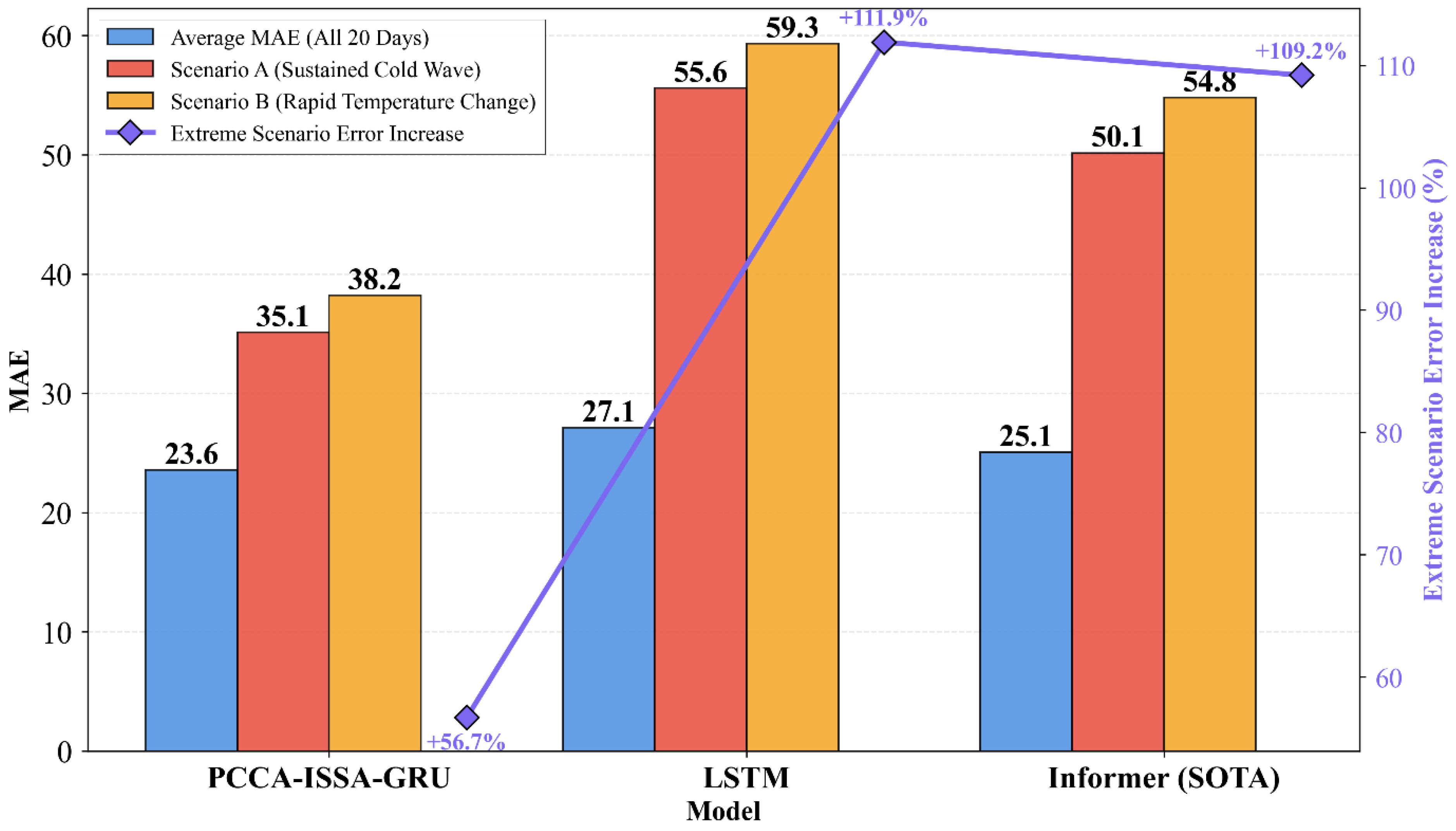
We then calculated the Mean Absolute Error (MAE) for the PCCA-ISSA-GRU model and the two primary comparison models (LSTM and Informer) across “All 20 Days” (average) and separately for these two “Extreme Scenario” subsets.

As shown in the MAE comparison results in Figure 22, under the average scenario, PCCA-ISSA-GRU achieved the lowest MAE (23.58). In Scenario A (Cold Snap) and Scenario B (Drastic Change), the errors for all models increased. However, the MAE for PCCA-ISSA-GRU (35.10 and 38.20) remained significantly lower than that of LSTM (55.60 and 59.30) and Informer (50.15 and 54.80). Furthermore, looking at the “Average Error Increase in Extreme Scenarios,” the error for PCCA-ISSA-GRU increased by only 56.7%, whereas the error amplification for both LSTM and Informer exceeded 100%.

This result demonstrates the superior robustness of the PCCA-ISSA-GRU framework. Standard deep learning models like LSTM and Informer are prone to “overfitting” or “panicking” when faced with extreme inputs (low temperatures or drastic temperature changes) that are uncommon in their training set, leading to severe deviations in their predictions.

Our model’s superior performance stems from its preprocessing:

(1)

The PCCA algorithm more clearly captures the core correlation between temperature and load. PCCA is effective because it re-sorts the principal components based on “correlation contribution,” ensuring the features input to the GRU are both orthogonal (from PCA) and target-relevant (from correlation analysis). This resolves the issue of redundant factors.

(2)

At the same time, ISSA provides statistics-based noise identification. By checking if a component approximates a Gaussian distribution (which typically represents random noise) using skewness and kurtosis, ISSA adaptively removes noise, rather than arbitrarily (as in standard SSA). This provides a “cleaner” signal for the GRU, allowing it to focus on learning the true load patterns.

PCCA provides “clean” external drivers, and ISSA provides a “clean” historical load signal. The combination of the two downgrades the GRU’s prediction task from “hard” mode to “simple” mode. This allows the GRU to make predictions on a more stable and cleaner data foundation, thereby maintaining higher reliability within the “tactical planning window” (10–20 days) and during critical high-risk moments.

This reliable forecast result provides Local Distribution Companies (LDCs) with the decision-making confidence needed to strike a balance between the “volatile spot market” and “limited contract/storage volumes.” It enables operators to make procurement decisions later (closer to the delivery date), thus better leveraging market price fluctuations while drastically reducing the risk of catastrophic financial consequences from “underestimating demand.”

5. Conclusions, Limitations, and Future Work

5.1. Conclusions

Addressing the issues of “information misalignment” in feature extraction and non-Gaussian noise interference prevalent in short-term urban gas load forecasting, this paper proposes a PCCA-ISSA-GRU hybrid framework designed for short-to-medium-term (10–20 days) natural gas load forecasting. By utilizing the PCCA algorithm, the framework resolves the issue of high multicollinearity among input features (particularly meteorological factors), ensuring both the orthogonality and high correlation of inputs. Simultaneously, through the ISSA algorithm, it utilizes statistical criteria such as skewness and kurtosis to adaptively identify and remove random high-frequency noise from historical load sequences.

Based on an empirical analysis of a real-world dataset from a major city in Northern China, the main conclusions are as follows:

(1)

Mechanism Effectiveness and Resolution of Pain Points: PCCA and ISSA effectively address the inherent defects of traditional methods. Traditional PCA, based on variance ranking, ignores subtle features strongly correlated with the load; PCCA retrieves this critical information through a correlation-based reconstruction mechanism. Meanwhile, ISSA achieves precise elimination of the non-Gaussian “spike” noise commonly found in gas data. Ablation experiments confirm that the combination of the two forms a complementary effect of “feature optimization” and “signal purification.”

(2)

Significant Accuracy Improvement and Marginal Benefit Analysis: Within the 10–20 day “tactical planning window,” the proposed model achieved the lowest prediction error (20-day MAPE of 6.09%). The marginal benefit analysis quantified the contribution of each module:

• Relative to the Benchmark: Compared to the unoptimized single GRU (MAPE = 31.00%), the model reduced the error by 80.35%.
• Relative to Traditional Improvements: Compared to PCA-GRU (MAPE = 25.50%), the introduction of PCCA further reduced the error by 76.12%. This figure directly proves the immense value of PCCA in salvaging “low variance but high correlation” features.
• Statistical Significance: The Diebold–Mariano test results indicate that the short-term prediction accuracy of this model is statistically significantly superior (p < 0.05) to all benchmark models, including BPNN, LSTM, GRU, ARIMA-ANN, and Informer.

(3)

Cost–Benefit Advantage Compared to SOTA Models: Although Transformer-based models (such as Informer) possess advantages in long-sequence forecasting, the PCCA-ISSA-GRU framework demonstrates higher practical value for the short-to-medium-term window (10–20 days) focused on in this study.

• Robustness Advantage: Under extreme weather scenarios such as continuous cold waves and drastic temperature changes (see Figure 22), the error increase of our model (+56.7%) was far lower than that of Informer (+109.2%), demonstrating its stability under small-sample fluctuations.
• Deployment Efficiency: Compared to the complex hyperparameter tuning and high computational demands of Informer, this framework offers shorter training times and more convenient tuning, making it a more cost-effective solution than complex SOTA models.

(4)

Commercial Value in Actual Operations: The contribution of this study lies not only in accuracy improvement but also in its significant operational implications. In the energy market, especially within the “tactical window,” the cost of forecast errors is non-linear and asymmetric. “Underestimating demand” may force gas companies to bear punitive high spot prices, while “overestimating demand” leads to unnecessary procurement and storage waste. Our model elevates prediction accuracy to the SOTA level while maintaining maximum reliability in critical extreme scenarios. This statistically verified improvement in accuracy and robustness provides key confidence for gas companies’ operational decisions, drastically reducing the risk of major financial losses caused by forecasting errors.

5.2. Limitations

Despite these positive results, this study has the following limitations:

(1)

Single Data Source: This study utilized a dataset from only one city. The model’s generalization capability (e.g., to industrial loads or different climatic zones) has yet to be validated.

(2)

Validation Strategy: We employed a fixed hold-out (back-testing) validation. Future work should adopt a more robust time-series rolling cross-validation to confirm the results.

(3)

SOTA Comparison: Although we included the Informer, we did not conduct a comprehensive comparison against the latest Foundation Models or other Transformer variants. This analysis will be further deepened in future research.

5.3. Prospects

This study focused on short-term urban gas load forecasting and has limitations in long-term prediction. Combining insights from previous research and future trends in predictive modeling, future studies can focus on the following aspects:

(1)

Further exploration of emerging technologies in NGLF. This study introduced deep learning networks into NGLF, showing clear advantages over classic models and the Informer model in the short term. However, it suffers from the error accumulation phenomenon in long-term forecasting. With the development of computer hardware, research in Large Language Models (LLMs) is rapidly advancing, and new predictive techniques are constantly emerging. How to apply LLMs to forecasting research to achieve intelligent long- and short-term prediction will become a new direction for future research.

(2)

Future research can be deepened at the mechanistic level (e.g., embedding physical constraints), the data level (e.g., constructing spatio-temporal graph neural networks), and the system level (e.g., establishing a Federated Learning-driven self-evolving framework). This will promote the forecasting paradigm to evolve from data-driven methods toward intelligent, knowledge-enhanced decision intelligence.