Interactions and Binding Energies in Carbon Nanotube Bundles

Abstract

On any size scale, it is important to know how strongly structural components are held together. The purpose of this work was to develop a means to estimate the collective binding energy holding together a bundle of aligned carbon nanotubes (CNTs). Carbon nanotubes in isolation and in bundles have unique and useful properties and applications within supramolecular structures and nanotechnology. Equations were derived to represent the total number of pairwise interactions between the CNTs found in various size and shape bundles. The shapes considered included diamond, hexagon, parallelogram, and rectangle. Parameters were used to characterize the size of a bundle for each defined shape. Force field molecular modeling was used to obtain the total bundle binding energies for a number of sample bundles. From the number of interactions per bundle, the binding energy per interaction was determined. This process was repeated for armchair CNTs having a range of length and circumference values. A simple equation described the interaction energy based on the length and circumference of the component armchair type nanotubes. When combined with the bundle shape and size parameters, the total bundle binding energy could be found. Comparison with whole bundle molecular mechanics calculations showed our formula-based approach to be effective.

1. Introduction

Carbon nanotubes (CNTs) exhibit remarkable tensile strength and high thermal conductivity. Their electrical properties can vary from high conductivity metallic to semiconductor depending on their configuration. There are a number of interesting properties, behaviors, and potential applications of both isolated carbon nanotubes, as well as collections of CNTs found in pure bundles or combined with other molecules or polymers to create more complex mixed nanostructures. Mechanical properties that utilize the advantages of the stiff sp² bonds within nanotubes, along with relatively weaker van der Waals (vdW) interactions between tubes, have been characterized by scanning probe microscopy and could give rise to nanoelectromechanical devices such as nanomotors, oscillators, or switches [1]. Two-dimensional patterns of single-walled carbon nanotube (SWCNT) bundles are scalable for utilization in devices and nanocomposites based on their unique optical, electrical, and mechanical properties that depend on not only isolated tube behaviors but also the collective behavior based on tube–tube interactions [2]. Other interesting properties and applications for CNT bundles are considered below.

Electrical properties have been examined. Bundles of double-walled carbon nanotube-composite material (CB-DWCNTs) have been studied for antenna applications at the terahertz frequency range [3]. The super aligned CNT (SACNT) array holds promise for use in lithium-ion batteries due to its unique electrical mechanic properties [4].

Thermal properties, including heat storage and transport, are of interest. The heat storage and output of a hybrid material consisting of magnesium hydroxide in carbon nanotube bundles was explored with consideration toward chemical heat pumps and improved heat storage [5]. The thermal conductivity of chemical-vapor-deposition-grown carbon nanotube bundles and the role of CNT defects was studied [6].

Sensor and surface properties have been studied. An artificial-hair-type sensor made from aligned CNT bundles has piezoresistive behavior with a detection sensitivity similar to that of hair sensors on insects and may have application in devices such as cochlear implants [7]. Surface nanostructures with the interesting application of an artificial gecko sole were formed by transferring carbon nanotube bundles to macromolecular tapes to give superior adhesion [8].

Sorption and adsorption properties have been investigated. Molecular dynamics simulations of CNT bundles for water purification and gas separation have been examined, along with molecular sieving and desalination in applications in nanoscale devices [9]. CNTs adsorbents for the removal of industrial dyes from wastewater were examined and related to the nature of adsorbate and adsorbent properties and interactions, such as vdW forces and hydrogen bonding [10]. Organic micropollutants’ removal from the environment may be based on adsorption on pristine CNTs or modified CNTs [11]. Oil removal from water was studied by using CNT bundles made by injected vertical chemical vapor deposition that created CNT bundles from 20 to 50 nm in diameter and with lengths of 300 to 500 μm. These bundles were effective in oil removal with possible application for oil spill cleanup [12].

Understanding the size, shape, and structure of self-assembled fiber bundles and aggregates is significant to problems in supramolecular structures and materials science [13]. The controlled growth of carbon nanotubes in isolation or with other materials via van der Waals forces, specific chemical interactions, DNA pairing, and functionalization gives potential applications utilizing self-assembly [14]. Computational models of the mechanical and transport properties were adjusted in CNT bundles by varying the degree of CNT alignment. Self-organization of CNTs fibers was based on bundle size and orientation [15].

The ability to engineer bundle sizes is essential for varied applications of CNTs, and, for that purpose, various sizes and types of CNT bundles have been grown from different-sized cobalt catalyst clusters with chemical vapor deposition [16]. A method of patterned CNTs synthesized was developed on silicon substrates by use of plasma-enhanced chemical vapor deposition and solution dipping deposition. CNT bundles in periodic structures could be adjusted based on concentration of solution and plasma conditions [17]. Different methods of generating multiwall carbon nanotubes (MWCNTs) revealed how the synthesis conditions can affect the nanotube structures and properties of the formed bundles [18]. Single-wall carbon nanotubes (SWCNTs) tend to aggregate into larger bundles, but a constant electric field applied during arc discharge created bundles where 98% were less than 10 nm in diameter and 50% were less than 3 nm in diameter [19]. 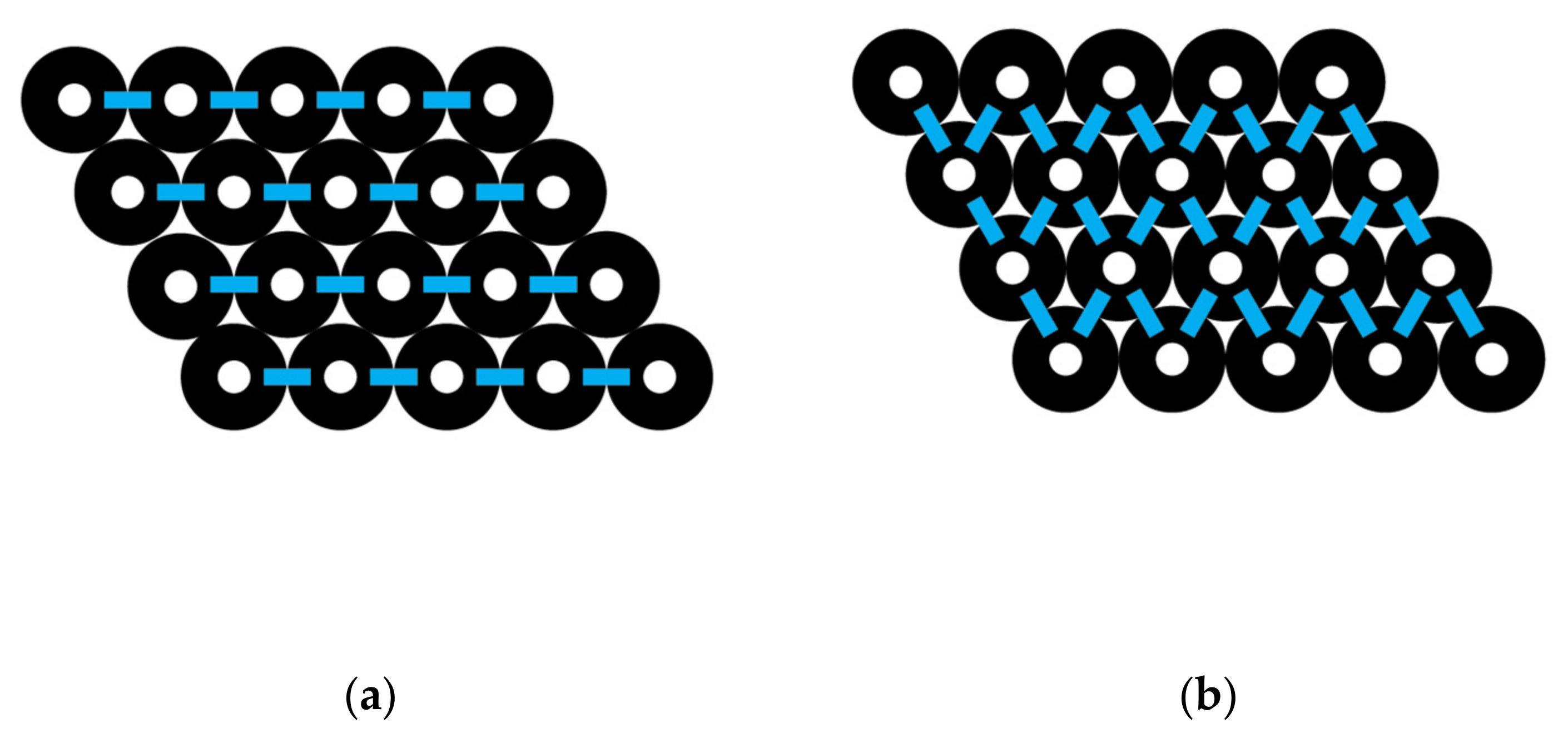Interactions among CNTs have been examined by experimental [20] and modeling methods [21,22]. In our own prior work using molecular mechanics, the difference between perpendicular and parallel structures of carbon nanotubes have been shown to significantly favor parallel structures [23]. Single-walled (5,5) CNTs with an internuclei diameter of 0.67 nm and an internuclei length of 4.46 nm (18 rings) were compared in perpendicular and parallel arrangements. Relative to the two isolated CNTs, the perpendicular arrangement gave a stabilization energy of −17.7 kcal/mol, and the parallel arrangement gave a stabilization energy of –83.1 kcal/mol [23]. Obviously, and as expected, the parallel orientation due to vdW forces is much more stable than the two isolated CNTs or than the two perpendicular CNTs.

Reported modeling work for two (5,5) CNTs at right angles gave a stabilization of 0.761 to 0.785 eV or 17.6 to 18.1 kcal/mol, in agreement with our results [24]. Stabilization in grouping of CNTs due to noncovalent interactions gives negative interaction energies if considered to be the formation of a stable structure made from its component parts. However, positive values may be reported as the energy required to disassemble or separate a structure into its component parts. CNT interactions have been examined computationally by various approaches, focusing on the dispersion forces of attraction [24,25,26,27,28,29]. Organic oligomer solvent systems have been modeled by several different dispersion-corrected density functional theory (D-DFT) approaches, including B97D, wB97XD, and B3LYP-D3 [30]. In this work, their interest was in the role of solvation and nanotube size on binding energies, electronic properties, and the structure of model compounds on segments of nanotubes [30].

Because of the large number of atoms involved in CNT bundle structures, molecular-mechanics force-field calculations can provide a useful method to determine the total binding energy between the CNTs that serves to hold the structure together. Molecular mechanics (MM) predicts the conformations of molecules or molecular structures through the optimization of atomic positions that minimizes steric energy. A molecule’s steric or conformational energy is the sum of its component energy contributions.

Different parameter and equation sets are optimized for different applications. The MM2 and MM3 sets were originally developed to optimize the structures of certain types of isolated organic molecules. MM2 force-field parameters include contributions from bond stretch, stretch–bend, bond angle, dihedral angle, improper torsion, van der Waals interactions, electrostatics, and hydrogen bonding. MM3 includes some additional terms. We have found both the MM2 and MM3 parameter sets to be effective in estimating surface vdW interactions.

In our prior work, it was shown that, in comparison to experimental values, molecular mechanics can provide extremely useful estimates of the molecule–carbon surface binding energies and carbon surface–carbon surface binding energies [23]. For 15 experimental binding energy values (∆E_exp) taken from the literature, the same adsorbate–adsorbent systems were modeled. Molecular mechanics, using MM3 parameters, was used to obtain calculated binding energies (∆E) for comparison. A linear regression plot of the experimental and calculated data points gave a plot with a correlation of R² = 0.931 for ∆E_exp = 1.037 ∆E.

Some reported density function theory (DFT) calculations have shown poor correlations with experimental values for interactions dominated by vdW interactions unless a dispersion correction was included. However, when DFT with dispersion-correction binding energies (∆E_DFT-corr) for 28 different adsorbate–adsorbent systems were compared to our molecular mechanics calculations for the same systems [23], we found a correlation of R² = 0.866 and a linear regression plot of ∆E_DFT-corr = 1.027 ∆E.

In other prior works, it was shown that MM2 parameters without modification provide appropriate binding energy values for rigid adsorbates dominated by sp² carbons. A graphite surface was modeled by three parallel layers of graphene, which was shown to be adequate in representing the surface and vdW adsorbate–adsorbent interactions [31]. Experimental values for 60 different molecule–graphite binding energies obtained from published gas–solid chromatography experimental values were plotted versus our molecular mechanics force field values for the same rigid molecules. A correlation of R² = 0.913 was associated with the linear regression ∆E_exp = 0.992 ∆E.

In other prior works, the effectiveness of MM2 force field parameters was demonstrated for monolayer molecule coverage of graphite by comparing experimental thermal desorption binding energy values to our calculated binding energy ∆E values for 14 different molecules, namely benzene, C₆₀ buckyball, coronene, 1,1-dichloroethane, ethanol, ethylbenzene, methane, methanol, naphthalene, N,N-dimethylformamide, o-dichlorobenzene, ovalene, toluene, and trichloromethane [32]. Taking into account molecule–molecule interactions, as well as molecule–graphite interactions, gave a R² = 0.967 correlation for ∆E_exp = 1.119 ∆E.

Since our interest is in computations of supramolecular systems with structures having thousands of atoms, and since molecular mechanics with MM2 parameters work well for binding energies of sp² carbon-based systems, this approach is used for modeling individual CNTs and a variety of CNT bundles. This method is computationally convenient, rapid, and effective. Our interest is in finding the interaction energies of adjacent CNT’s for a range of circumferences and lengths and converting the calculated values to an equation-based representation of the binding energies.

These interaction energies must be combined with the number of CNT–CNT interactions within a bundle to determine the total binding energy holding a bundle together as one supramolecular system. Considerations of bundle shape and size should lead to simple equations to predict the number of interactions within defined bundle shapes including diamond, hexagon, parallelogram, and rectangle. Our results are based on an idealized model in which there is a regular hexagonal packing arrangement of perfectly aligned CNTs and there is no collapse of the walls in the larger CNTs.

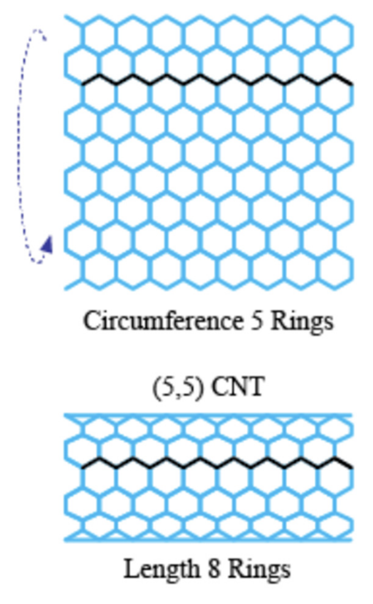
Although they are not formed in this manner, the different configurations can be understood by imaging rolling a single layer of hexagonal graphene containing only sp² hybridized carbons into a tube, as shown in Figure 1. In this work, our consideration of CNT bundles is limited to ones made of identical tubes all having an armchair configuration. This armchair configuration corresponds to rolling the graphene image shown in Figure 1 downward to form a nanotube. The type of CNT is given by a (n, m) specification, where n and m are integer values. In the armchair configuration, n = m, as distinguished from the zigzag or chiral forms.

Our models are limited to single-wall carbon nanotubes that are not capped at either end. Within these restrictions, rather than considering the diameter and length directly, it is possible to define a unique armchair CNT by specifying the circumference in terms of the number of benzene rings or the equivalent number of phenyl-type-connected groups going around the tube. In addition, the length of the tube can be specified in terms of the number of hexagonal rings along the axis of the tube. A (5,5) CNT is shown (see Figure 1) that has five rings in circumference and eight rings in length.

A more universal representation would be based on the diameter and specific the chirality of the CNTs used in a bundle. For simplicity and to illustrate the interaction summation equations that are developed, our model is limited to the armchair type of CNT and thus uses a simple notation to specify the armchair CNT circumference and length.

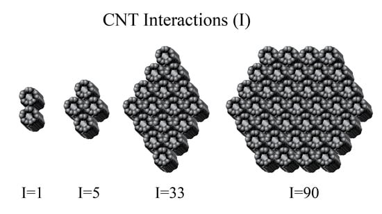
Since CNT bundles may have significant roles in supramolecular structures, it would be advantageous to be able to quickly estimate the stabilization energy among various sizes and shapes of CNT bundles. In addition to the number of interactions among a bundle, it will be useful to show that simple equations can be used to estimate the individual interaction energy based on the building block CNTs used to construct a specific bundle.

The purpose of this work was as follows: first, to derive formulas for the number of pair CNT–CNT interactions (I) for a given shape and size bundle; second, to determine a formula for the interaction energy between CNT pairs based on the CNT length and circumference; third, to combine to the two component parts to be able to easily estimate the overall bundle binding energy (ΔE); and fourth, to confirm that this equation approach gives appropriate estimates of ΔE when compared to direct force-field calculations from using MM2 and Equation (1). It is appreciated that a formal-based estimate of ∆E would be quicker, simpler, and more versatile than having to calculate ∆E for every specific bundle of interest.

2. Methods

Scigress (Fujitsu), molecular modeling software, was used to study the noncovalent interactions among bundles of carbon nanotubes. The carbon nanotubes remain in stable structures, but the energy of a collection of CNTs is modified as they are brought together. The overall energy is lowered primarily due to vdW interactions. All energies were calculated by using the MM2 force-field parameters.

To compare the stabilities of structures, it is necessary to compare the noncovalent binding energies among a CNT structure, due to vdW forces relative to its component parts of isolated CNTs. A structure’s overall binding energy (ΔE) that holds a collection of CNTs together can be calculated by finding the sum of the individual component energies (E_a + E_b + E_c + …) and subtracting from this value the energy of the combined structure or E(CNT bundle). The structures of interest for this study are aligned bundles of parallel CNTs whose energy is given by E(CNT bundle). The binding energy that holds the structure together (∆E) is given by the following:

ΔE = (E_a + E_b + E_c + …) − E(CNT bundle)

(1)

As written in Equation (1), the ∆E will be a positive value or the energy that must be put into a system to separate the bundle of CNTs into all its separate parts. The energy of the bundle is lower in energy than the separate CNTs because of the stabilization due to vdW forces between adjacent nanotubes.

Our objective was to develop simple formulas that could be used to estimate the total binding energy within a bundled collection of CNTs. The binding energy, ∆E, depends on the shape and size of the bundle, since that determines the total number of interactions among touching CNTs. The noncovalent binding energy that is associated with the single interaction between any pair of touching armchair nanotubes (∆E₁) depends on the length and the circumference of the individual CNTs that compose the bundle and make up each pair interaction.

Figure 2 shows four groupings of CNTs. One of these groups is a simple pair of two CNTs with one CNT–CNT interaction between them. This interaction is based on the vdW attraction that causes the pair to be at a lower energy than the two isolated CNTs. The interaction is based on the linear region of contact between the two CNTs. Another group of four CNTs is shown, and this group has a total of five interactions. This group has a greater stabilization energy or collective group binding energy than the pair. A diamond-shaped bundle composed of 16 CNTs is shown, and it has 33 unique pair interactions. These interactions can be counted, but a simpler formula-based approach for all similar-shaped bundles is derived. Finally, the end view of hexagonal-shaped bundle containing 37 CNTs is shown. This hexagonal bundle has 90 unique CNT–CNT pair interactions. Formula-based approaches to determine the number of interactions were derived for all similarly shaped bundles.

3. Analysis and Results

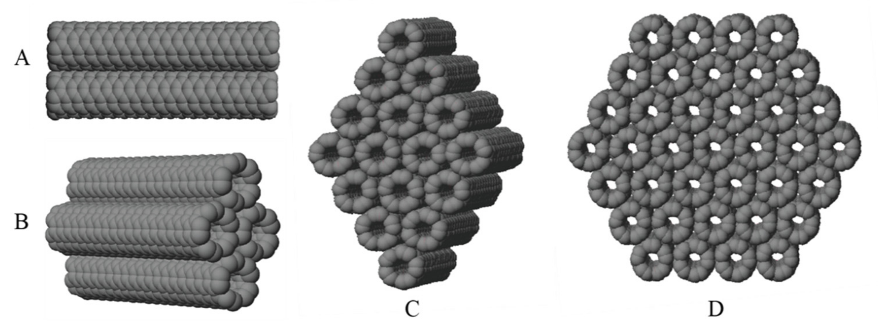
The shape of any CNT bundle is based on the arrangement of the individual CNTs. To illustrate this effect, four basic bundle shapes are considered, namely diamond, hexagon, parallelogram, and rectangle. These shapes, as we define them, are illustrated in Figure 3, Figure 4, Figure 5, Figure 6, respectively, and are discussed below. In each case, a few parameters define the size and shape of the bundle, and these parameters are used to develop equations that can predict the number of CNT–CNT pair interactions, I, within each specific bundle. Other bundle shapes are possible—for example, a triangle—but these four were the specific ones considered.

3.1. Diamond CNT Bundle Interactions

For a diamond-shaped CNT bundle (Figure 3), let N₀ represents the number of carbon nanotubes in the 0th or central layer, which is the layer with the largest number of CNTs. A counting index, i, is used to refer to different layers so that, for example, i = 1 represents the pair of layers above and below the central layer and N₁ the number of CNTs in that layer. In the specific example shown, N₀ = 4 and N₁ = 3. L is the maximum number of paired layers in the complete diamond-shaped CNT bundle. Thus, above and below layer 0 is layer 1 where N₁ = N₀ − 1. Above and below layers 1 are layers 2, where N₂ = N₀ − 2. Above and below layers 2 are layers 3, where N₃ = N₀ − 3, and so forth. In a complete diamond shape, the highest and lowest layer is i = L, where L = N₀ − 1. The number of CNTs in layer L is designated as N_L, and N_L would have a value of 1.

The number of interactions across any layer will always be one less than the number of CNTs in that layer, since the interactions are between each pair of CNTs. Therefore, the total number of CNT to CNT across interactions among all the layers, I_across, is given by the following:

$${\mathrm{I}}_{\mathrm{across}} = ({\mathrm{N}}_0 -1)+2 {{\displaystyle \sum }}_{i=1}^{\mathrm{L}}(({\mathrm{N}}_0 - i) - 1)$$

(2)

where the counting index has a maximum value of L. N₀ − 1 represents the number of interactions in the central layer, and the summation is the number in all the other layers which is multiplied by 2, since there is a top and bottom of diamond shape to consider. For example, the number of interactions going across the specific bundle illustrated in Figure 3 can be found, since N₀ = 4, L = 3. Using Equation (2), we get the following:

I_across = (4 − 1) + 2 [((4 − 1) − 1) + ((4 − 2) − 1) + ((4 − 3) − 1)]

which is equal to the expected 9 interactions going across.

Now the number of interactions going down the layers must be considered. The number of interactions from the top of the diamond going down is two times the number of CNTs per layer, since every CNT touches two CNTs below it (Figure 3). The interactions on the top half are as follows:

I_down (top) = 2N₁ + 2N₂ + 2N₃ …. + 2N_L

(3)

where the interactions going down per layer are equivalent to 2 times the number of CNTs in each layer. If we redefine in terms of the number of CNTs in the N₀ layer, then since N₁ = N₀ – 1, N₂ = N₀ – 2, N₃ = N₀ − 3, and so forth, we can write the following:

$${\mathrm{I}}_{\mathrm{down}}(\mathrm{top})={{\displaystyle \sum }}_{i=1}^{\mathrm{L}}2({\mathrm{N}}_0 - i)$$

(4)

This equation must be multiplied by 2 to account for both the top half and bottom half interactions, which give the total down interactions as I_down, where I_down = I_down(top) + I_down(bottom) or

$${\mathrm{I}}_{\mathrm{down}}=4 {{\displaystyle \sum }}_{i=1}^{\mathrm{L}}({\mathrm{N}}_0 - i)$$

(5)

where i represents the layers (i = 1, 2, 3…L) of the CNT diamond-shaped bundle. To illustrate a specific example, the total number of interactions going down the diamond-shaped CNT bundle in Figure 3, where L = 3 and N₀ = 4, is given by Equation (5), where we get the following:

I_down (total) = 4 [3 + 2 + 1 + 0],

which is equal to 24 down interactions.

To get the total number of interactions in a diamond-shaped bundle, I(diamond), Equations (2) and (5) are combined, since the interactions are either across or down so that we have the following:

I(diamond) = I_across + I_down

(6)

and this gives the following:

$$\mathrm{I}\left(\mathrm{Diamond}\right) = ({\mathrm{N}}_0 - 1)+2 {{\displaystyle \sum }}_{i=1}^{\mathrm{L}}(({\mathrm{N}}_0 - i) -1)+4 {{\displaystyle \sum }}_{i=1}^{\mathrm{L}}({\mathrm{N}}_0 - i).$$

(7)

Separating the summations above into separate parts gives the following:

$$\mathrm{I}(\mathrm{diamond}) = ({\mathrm{N}}_0 - 1)+2 {{\displaystyle \sum }}_{i=1}^{\mathrm{L}} {\mathrm{N}}_0 - 2 {{\displaystyle \sum }}_{i=1}^{\mathrm{L}}i - 2 {{\displaystyle \sum }}_{i=1}^{\mathrm{L}}1+4 {{\displaystyle \sum }}_{i=1}^{\mathrm{L}}{\mathrm{N}}_0 - 4 {{\displaystyle \sum }}_{i=1}^{\mathrm{L}}i$$

(8)

and simplifying this equation gives the following:

$$\mathrm{I}\left(\mathrm{diamond}\right) = ({\mathrm{N}}_0 - 1) + 2 \mathrm{L} {\mathrm{N}}_0 - 2 {{\displaystyle \sum }}_{i=1}^{\mathrm{L}}i - 2 \mathrm{L} + 4 \mathrm{L} {\mathrm{N}}_0 - 4 {{\displaystyle \sum }}_{i=1}^{\mathrm{L}}i$$

(9)

Next, combining like terms gives the following:

$$\mathrm{I}(\mathrm{diamond}) = 6 \mathrm{L} {\mathrm{N}}_0 - 6 {{\displaystyle \sum }}_{i=1}^{\mathrm{L}}i+{\mathrm{N}}_0 –1 - 2 \mathrm{L}$$

(10)

The summation below is known as the “triangular number sequence” and is given by the following:

$${{\displaystyle \sum }}_{i=1}^{n}i=\frac{1}{2}{n}^2 +\frac{1}{2}n$$

(11)

For example, if n = 4, then from above 1 + 2 + 3 + 4 = 10 and (½) 4² + (½) 4 = 10. Using Equation (11), where L is used in place of n and then substituting into Equation (10), gives the following:

$$\mathrm{I}(\mathrm{diamond}) = 6 \mathrm{L} {\mathrm{N}}_0 - 6 [\frac{1}{2} {\mathrm{L}}^2+\frac{1}{2} \mathrm{L}]+{\mathrm{N}}_0 - 1 - 2\mathrm{L}$$

(12)

or

I(diamond) = 6 L N₀ − 3 L² − 3L + N₀ − 1 − 2L

and combining like terms gives the total number of interactions in a CNT diamond bundle arrangement as follows:

I(diamond) = 6 L N₀ − 3 L² − 5 L + N₀ − 1

(13)

To illustrate the application of this general equation, consider the specific example shown in Figure 3, where L = 3 and N₀ = 4, and substituting into the above gives the following:

I(diamond) = 6 (3) (4) − 3 (3) ² − 5 (3) + (4) − 1 = 33

(14)

which matches a direct count of the total number of interactions.

For a truncated diamond-shaped CNT bundle where L is less than the maximum allowed, the same formula is appropriate. To illustrate a specific example, if the bottom and top CNTs are removed (Figure 3), then L = 2 and N₀ = 4, and Equation (13) gives I(diamond) = 6 (2) (4) − 3 (2) ² − 5 (2) + (4) − 1 = 29. This result is expected, as we removed two top interactions by removing the single top CNT and removed two bottom interactions by removing the single bottom CNT. The equation for the total number of interactions for a diamond-shaped bundle with the knowledge of the outermost layer number (L) and the number of carbon nanotubes in the center of the bundle (N₀) is given by Equation (13) and applies for a complete diamond or one truncated at any number of layers, L, where the top and bottom form less than the maximum number of possible layers.

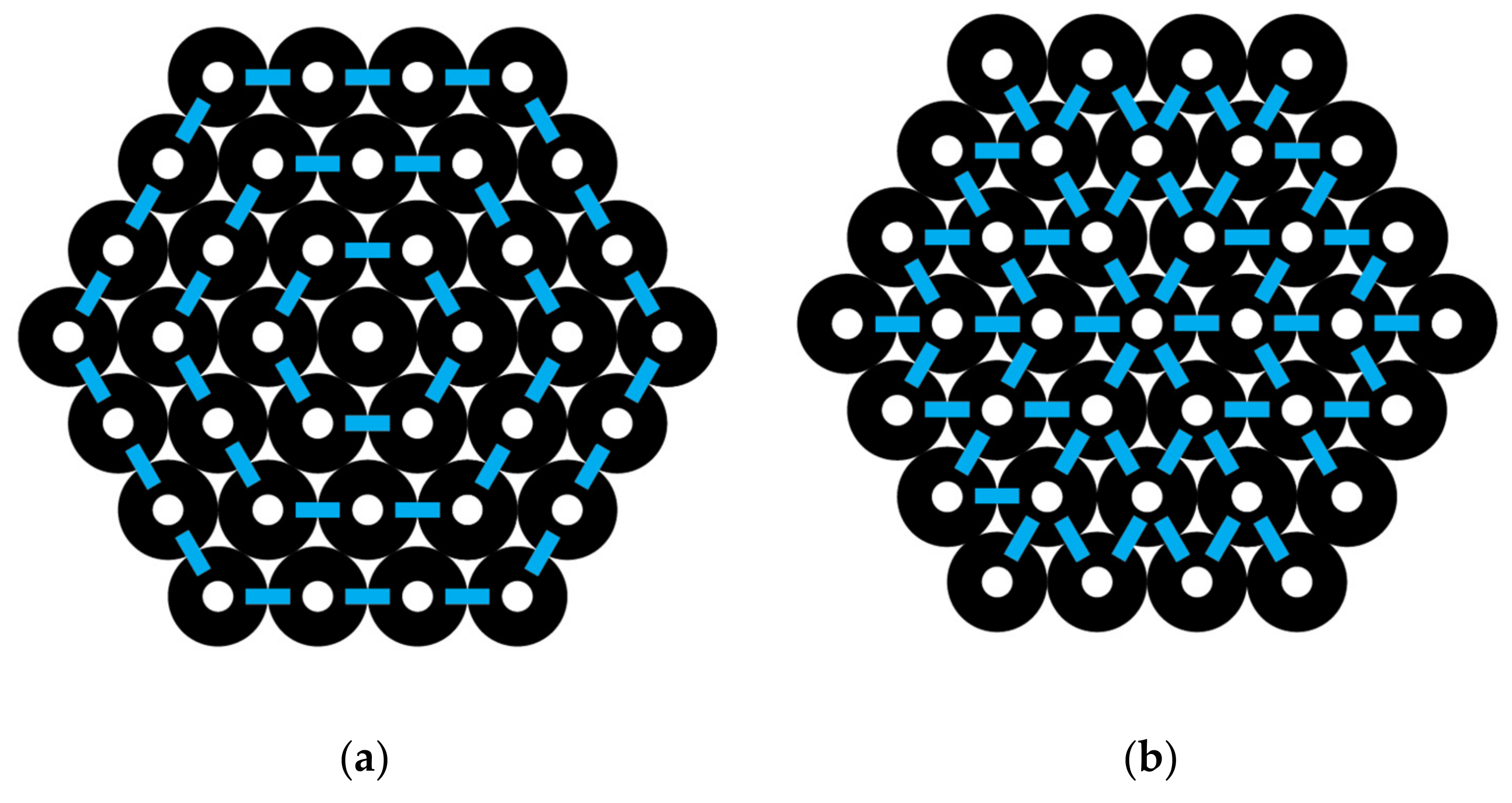
3.2. Hexagon CNT Bundle Interactions

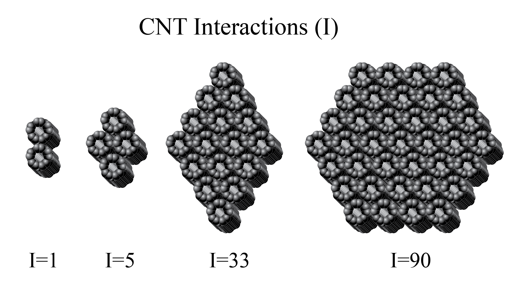
A hexagon-shaped bundle of CNTs is shown in Figure 4. If the central CNT is labeled as 0, then the ring layers around it going outward may be labeled successively as ring layer 1, 2, 3, etc. The numbers of CNTs in each ring layer, as shown in Figure 4, are N₀ = 1, N₁ = 6, N₂ = 12, and N₃ = 18. In general, the number of CNTs in each ring layer, I, beyond the one central CNT is N_i = 6i. The number of interactions around each ring layer is identical to the number of CNTs, N_i, in that layer, since there is an interaction between each pair. The total number of interactions around all the ring layers, using i as a counting index, 1, 2, 3, and up to L, the outermost ring in the CNT bundle, gives the following:

$${\mathrm{I}}_{\mathrm{around}}={{\displaystyle \sum }}_{i=1}^{\mathrm{L}}6i$$

(15)

For example, by using Figure 4, we can count the total number of interactions going around the successive ring layers of a hexagon-shaped CNT bundle, where L = 3 is the outermost layer, and observe from Equation (15) that I_around = (6 × 1) + (6 × 2) + (6 × 3) = 36 interactions.

In Figure 4, we can observe the interactions going out from an inner to an outer layer. Note that the number of interactions going outward between each layer is 6 for layers 0 to 1, 18 for layers 1 to 2, and 30 for layers 2 to 3. This sequence is fit by the formula 12 i − 6 as i varies from 1, 2, 3, and so forth. Thus, I_out for all the outward interactions is given by the following:

$${\mathrm{I}}_{\mathrm{out}}={{\displaystyle \sum }}_{i=1}^{\mathrm{L}}\left(12i –6\right)$$

(16)

For L = 3, the total interactions out are 6 + 18 + 30 = 54.

To get the total number of interactions in a hexagon-shaped bundle, I(hexagon), Equations (15) and (16) are combined, since the interactions are either around or out, so that we have the following:

I(hexagon) = I_around + I_out

(17)

and this gives the following:

$$\mathrm{I}(\mathrm{hexagon})={{\displaystyle \sum }}_{i=1}^{\mathrm{L}}\left(18i-6\right)$$

(18)

For example, if L = 3, then the total interactions are as follows:

I(hexagon) = (18 × 1 − 6) + (18 × 2 − 6) + (18 × 3 − 6)

which gives 90 as expected based on the direct counts for L = 3 of

I_around = 36 and I_out = 54

To simplify the prior equation, it may be written as follows:

$$\mathrm{I}(\mathrm{hexagon})=18 ({{\displaystyle \sum }}_i^{\mathrm{L}}i) - {{\displaystyle \sum }}_{i=1}^{\mathrm{L}}6$$

(19)

and using the “triangle number sequence” from Equation (11), then we get the following:

$$\mathrm{I}(\mathrm{hexagon})=18 (\frac{1}{2} {\mathrm{L}}^2 +\frac{1}{2}\mathrm{L}) - 6\mathrm{L}$$

(20)

Combing like terms gives the following:

I(hexagon) = 9L² + 3L

(21)

This equation predicts the total number of interactions in a hexagon CNT bundle and only requires knowing the total number of layers L. For example, if L = 3, then using the above gives I(hexagon) = 9 (3)² + 3 (3) = 90, which matches a direct count of the number of interactions given previously and shown in Figure 4.

3.3. Parallelogram CNT Bundle Interactions

A parallelogram-shaped CNT bundle is shown in Figure 5, where each layer has the same number of carbon nanotubes. L represents the total number of layers and N represents the number of carbon nanotubes in each layer. The total number of interactions across a given layer is given by I_across. Since there are N − 1 interactions per layer containing N CNTs and L layers, we can write the following:

I_across = L (N − 1)

(22)

For example, to calculate the total number of interactions going across the parallelogram-shaped CNT bundle shown in Figure 5, since L = 4 and N = 5, then I_across = 4 (5 − 1) = 16 interactions across the bundle.

To calculate the total number of interactions for each layer going down the CNT bundle, consider that the number of layers with down interactions is L − 1. All the CNTs except one per layer will have two down interactions, so that is 2(N − 1). The remaining CNT on one end of the layer will have just one interaction down. Therefore, the total down interactions are as follows:

I_down = (L − 1) [2 (N − 1) + 1]

(23)

Simplifying Equation (23) gives the following:

I_down = (L − 1) (2N − 1)

(24)

where L represents the layers in the CNT bundle and N represents the number of carbon nanotubes in each layer. For example, using Figure 5, where L = 4 and N = 5, the equation above gives I_down = (4 −1) [2(5) − 1] or 27 interactions.

Combining I_across and I_down from Equations (22) and (24) gives the total number of interactions in a parallelogram CNT bundle as follows:

I(parallelogram) = L (N − 1) + (L − 1) (2N − 1)

(25)

or simply

I(parallelogram) = 3LN − 2L − 2N + 1

(26)

For Figure 5 where L = 4 and N = 5, the total interactions are as follows:

I(parallelogram) = 3(4)(5) − 2(4) − 2(5) + 1

or 43 interactions.

This number matches the prior counts of 16 and 27 given above for this specific example.

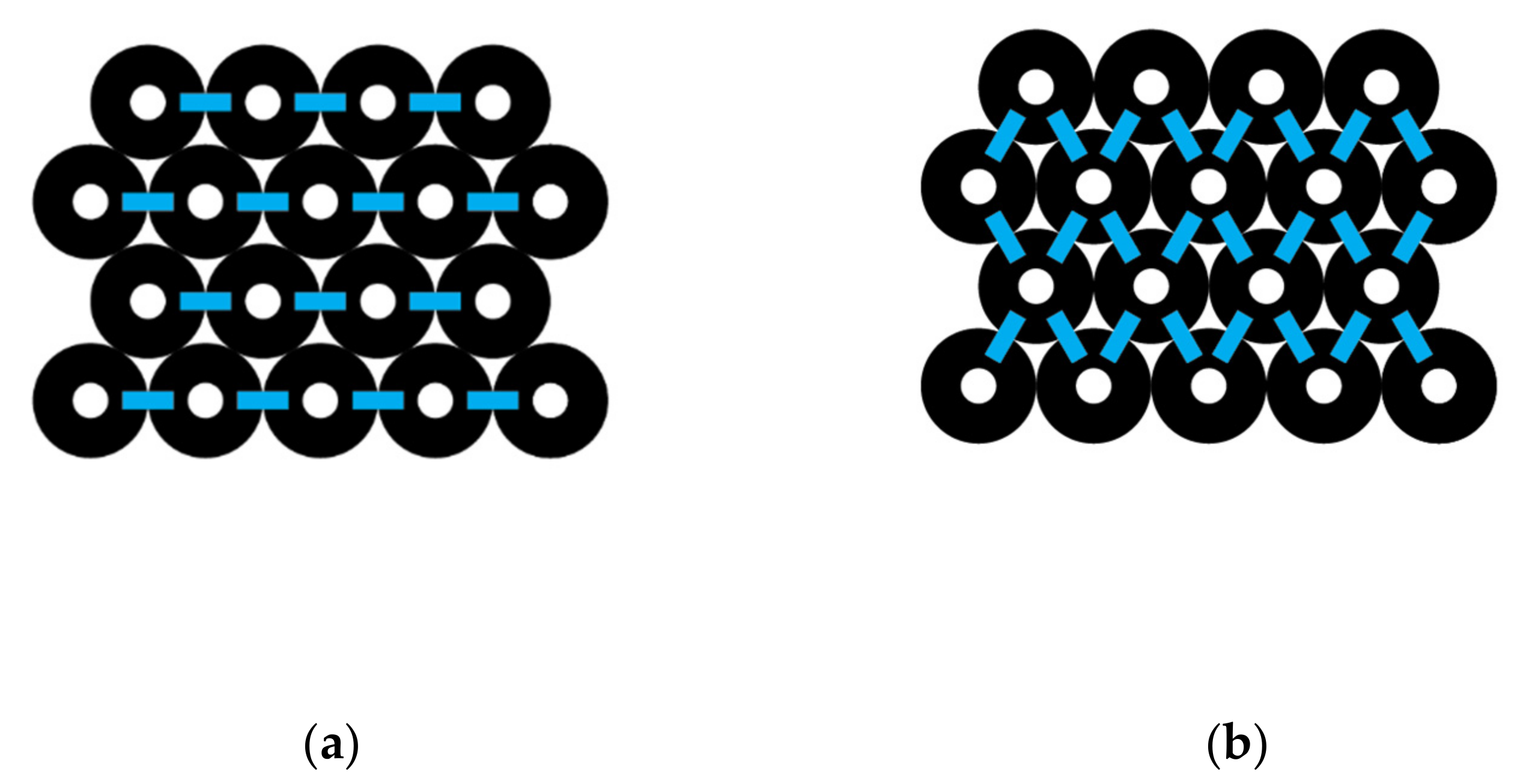
3.4. Rectangle CNT Bundle Interactions

A rectangle-shaped carbon nanotube bundle (Figure 6) is here defined as having alternating layers of CNTs that differ in number across by one. The top layer number is represented by N_a, and the next layer is represented by N_b, where we get the following:

N_a = N_b + 1,

(27)

and this alternating pattern repeats.

The total number of interactions going across a N_a layer is given as I_a and across a N_b layer is given as I_b. L represents the total number of layers in this CNT bundle. Therefore, the total interactions across all the “a” layers and all the “b” layers are as follows:

$${\mathrm{I}}_{\mathrm{a}} (\mathrm{for} \mathrm{all} {\mathrm{N}}_{\mathrm{a}} \mathrm{layers})=\frac{\mathrm{L}}{2} ({\mathrm{N}}_{\mathrm{a}} - 1)$$

(28)

and

$${\mathrm{I}}_{\mathrm{b}} (\mathrm{for} \mathrm{all} {\mathrm{N}}_{\mathrm{b}} \mathrm{layers})= \frac{\mathrm{L}}{ 2} ({\mathrm{N}}_{\mathrm{b}} - 1)$$

(29)

The number of interactions going across all layers (N_a and N_b) is the sum of the above:

$${\mathrm{I}}_{\mathrm{across}}=\frac{\mathrm{L}}{2} ({\mathrm{N}}_{\mathrm{a}} - 1)+\frac{\mathrm{L}}{2} ({\mathrm{N}}_{\mathrm{b}} - 1)$$

(30)

For example, the number of interactions going across the CNT bundle shown in Figure 6 is based on L = 4, and the number in each type of layer is N_a = 5 and N_b = 4. Substituting into the equation above gives I_across = 14 total interactions across.

To represent the total number of interactions going down, I_down, note that the number of layers to consider will be 1 less than the number of layers L. In addition, each region of contact between layers will have 2(N_a – 1) interactions, starting with the top layer (Figure 6). Therefore, the total number of down direction interactions is as follows:

I_down = (L − 1) [ 2(N_a − 1)]

(31)

For example, the total number of interactions down (Figure 6), where L = 4, N_a = 5, and N_b = 4, is as follows:

I_down = (4 − 1) [2 (5 − 1)] = 24

For the total number of interactions within a rectangle CNT bundle, combining I_across and I_down from Equations (30) and (31) gives the following:

$$\mathrm{I}(\mathrm{rectangle})=\frac{\mathrm{L}}{2} ({\mathrm{N}}_{\mathrm{a}} - 1)+\frac{\mathrm{L}}{2} ({\mathrm{N}}_{\mathrm{b}} - 1)+(\mathrm{L} - 1) (2{\mathrm{N}}_{\mathrm{a}} - 2)$$

(32)

or equivalently

$$\mathrm{I}(\mathrm{rectangle})=\frac{\mathrm{L}}{2} {\mathrm{N}}_{\mathrm{a}} - \frac{\mathrm{L}}{2} + \frac{\mathrm{L}}{2} {\mathrm{N}}_{\mathrm{b}} - \frac{\mathrm{L}}{2} +2 \mathrm{L} {\mathrm{N}}_{\mathrm{a}} - 2\mathrm{L} - 2{\mathrm{N}}_{\mathrm{a}}+2.$$

(33)

Combining like terms and simplifying gives the following:

$$\mathrm{I}(\mathrm{rectangle})=\frac{5\mathrm{L}}{2} {\mathrm{N}}_{\mathrm{a}} - 3\mathrm{L}+\frac{\mathrm{L}}{2} {\mathrm{N}}_{\mathrm{b}} - 2{\mathrm{N}}_{\mathrm{a}}+2.$$

(34)

Since N_a = N_b + 1, then Equation (34) becomes the following:

$$\mathrm{I}(\mathrm{rectangle})=\frac{5\mathrm{L}}{2} ({\mathrm{N}}_{\mathrm{b}}+1) -3\mathrm{L}+\frac{\mathrm{L}}{2} {\mathrm{N}}_{\mathrm{b}} - 2({\mathrm{N}}_{\mathrm{b}}+1)+2$$

(35)

Combining the like terms and simplifying gives the following:

$$\mathrm{I}(\mathrm{rectangle})=3{\mathrm{LN}}_{\mathrm{b}} - \frac{\mathrm{L}}{2} - 2{\mathrm{N}}_{\mathrm{b}}$$

(36)

for the total number of interactions for a rectangle-shaped CNT bundle. For example, the total number of interactions in Figure 6, where L = 4 and N_b = 3, becomes I(rectangle) = 3 (4) (4) − 4/2 − 2(4) = 38, which matches a direct count of the total number of interactions.

Other shapes could be defined, but these four illustrate that formulas based on these well-defined shapes need only parameters to indicate the size of the shape with regard to however the shape is defined to calculate the number of CNT–CNT interactions in a CNT bundle. Thus, Equations (13), (21), (26), and (36) predict the number of interactions in diamond (full or truncated), hexagon, parallelogram, and rectangle bundles, respectively.

For the calculations of bundle binding energy, it is the number of interactions that is essential to know and not the number of CNTs. However, the number of CNTs (n) for each of the four shapes are given by the following equations:

n(diamond) = L N₀

(37)

n(hexagon) = 3 L² + 3 L + 1

(38)

n(parallelogram) = L N

(39)

n(rectangle) = L N_b + L/2

(40)

The related equations for I are found in Equations (13), (21), (26), and (31). When each of these equations for I is divided by the corresponding equation above for n and taken to the limit of large n, then the lower order terms drop out and each shape gives a ratio of I/n = 3. As the number of CNTs becomes very large, a limit is approached where each CNT would have six nearest neighbors in a hexagonal packing arrangement, and since every interaction represents a pair of CNTs, then the ratio of I/n approaches a limit of 3.

An example of the above trend can be illustrated with the hexagon shape. Consider the trend where L = 1, 2, 3, 4, and 5. Then, Equation (21) for I(hexagon) = 9L² + 3L gives 12, 42, 90, 156, and 240 interactions, respectively. After that, Equation (38) gives for n(hexagon) = 3L² + 3L + 1 gives 7, 19, 37, 61, and 91, respectively. The associated ratios of I/n are approximately 1.714, 2.211, 2.432, 2.557, and 2.637. However, for larger bundles where the layers are L = 20, 40, and 100, the I/n ratios are approximately 2.902, 2.951, and 2.980, respectively. We observe the approach to the limit of I/n = 3 as n gets large. For example, for L = 100, there are 90,300 interactions and 30,301 CNTs.

3.5. Interaction Energy and Circumference

To characterize and easily be able specify different shapes and sizes of the CNTs, we had to establish how we define an interaction between groups of CNTs and how the circumference and length were assigned. A CNT interaction as noted previously is defined as the touching from any other neighboring CNT along two identical and aligned CNTs. The interaction count between two touching CNTs would be one interaction or I = 1. The CNT circumference (C_r) is defined as the number of phenyl rings that can be counted around the top of the CNT. For example, a (5,5) CNT has a circumference of C_r = 5. The CNT length (Z_r) is defined as the number of rings that can be along the axis of a carbon nanotube structure (see Figure 1).

To explore the role of CNT circumference, parallel bundle models were created consisting of 7, 8, 9, 10, and 11 single-walled carbon nanotubes. All the CNTs used in these bundles had a length of 14 rings or Z_r = 14. For convenience and easier visualization, the length of the CNTs used were defined by the number of rings (Z_r) from one end to the other along a line rather than a measurement expressed in nanometers. All CNTs used were based on the armchair configuration and included (4,4), (5,5), (6,6), (7,7), (8,8), (9,9), (10,10), (11,11), (12,12), (13,13), (14,14), and (15,15) CNTs. The bundles of 7, 8, 9, 10, and 11 CNTs had 12, 14, 16, 19, and 21 total CNT–CNT interactions, respectively.

For each bundle the energy required to disassemble the bundle or ∆E(bundle) can be calculated from Equation (1) or alternatively may be written as follows:

∆E(bundle) = n E_CNT − E(bundle)

(41)

where n is the number of CNTs, E_CNT is the energy of one CNT, and E(bundle) is the energy of the intact bundle of CNTs. This total bundle binding energy is the sum of all the individual noncovalent interactions present. The total interaction energy divided by the number of interactions gives the average single interaction per pair of CNTs or ∆E₁. For example, the MM2 steric energy of one isolated (4,4) CNT with Z_r = 14 was 790.14 kcal/mol. The bundle made of 10 (4,4) CNTs had a total MM2 steric energy of 7056.41 kcal/mol. The MM2 energy of the bundle subtracted from the MM2 energy of the 10 isolated CNTs gives the following:

∆E(bundle) = 10 (790.140) − 7056.41 = 844.99 kcal/mol

(42)

The ∆E(bundle) value of 844.99 divided by the 19 interactions present in that specific bundle of 10 CNTs gives 44.4 kcal/mol per interaction. This interaction energy is the noncovalent attraction between two contacting parallel CNTs where Z_r = 14. The energy for this single CNT–CNT interaction is ∆E₁ = 44.5 kcal/mol.

Three trials were completed for each of the five different bundle arrangements for each value of C_r. For a given CNT circumference, 15 values of ∆E₁ were obtained. This process of three duplicate measurements for each five different bundles was repeated for each of the 12 different C_r values, with CNTs ranging from the smallest (4,4) CNT to the largest (15,15) CNT.

Table 1. CNT–CNT binding-energy values, ∆E₁ (kcal/mol), from CNT bundles and CNT pairs as circumference of component nanotube measured in rings (C_r) were varied. Ratio of ∆E₁ values obtained from bundles and from simple pairs indicates agreement between methods.

Circumference	∆E1(kcal/mol)	∆E1(kcal/mol)	Ratio ∆E1
Cr (Rings)	Bundle	Pair	Bundle/Pair
4.00	44.40	45.89	1.03
5.00	47.40	46.70	0.99
6.00	52.30	51.62	0.99
7.00	56.30	56.32	1.00
8.00	62.80	62.52	1.00
9.00	64.80	65.00	1.00
10.00	68.80	70.28	1.02
11.00	72.40	73.55	1.02
12.00	75.90	75.05	0.99
13.00	79.90	79.46	0.99
14.00	83.50	83.42	1.00
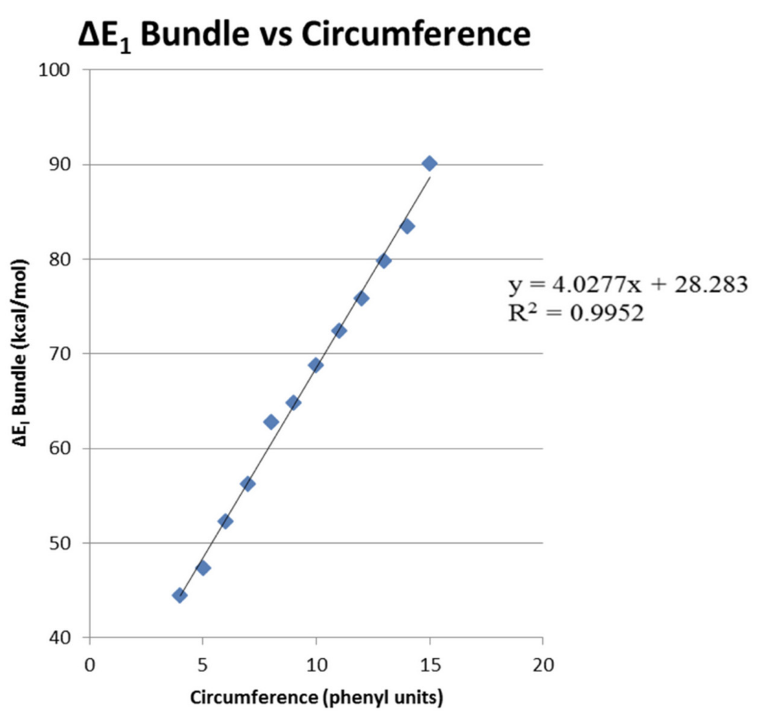
15.00	90.10	92.27	1.02

summarizes the results by giving the average binding energy per one interaction for each of the different CNT circumference.

The results for ∆E₁ ranged from 44.4 to 90.1 kcal/mol for CNT C_r = 4 to C_r = 15. Figure 7 shows a plot of the average binding energy per CNT–CNT interaction values from Table 1 versus the circumference expressed as C_r values from 4 to 15. The best fit linear equation for this plot of ∆E₁ versus C_r was as follows:

∆E₁ = 4.028 C_r + 28.28

(43)

with an R² = 0.995 value.

For comparison, simple pairs were assembled for each of the varied CNT circumferences from (4,4) to (15,15). Each aligned pair was constructed three times, and the three trials done for each different circumference were averaged. These average results are summarized in Table 1. The results confirm that the pair interaction, as expected, provides a close representation of the average interaction energy obtained from the bundle. A best fit linear equation for the plot of ∆E₁ versus C_r was found to give the following:

∆E₁(pair) = 4.040 C_r + 28.57

(44)

and R² = 0.988 value. This equation based on pairs closely matches the bundle results and confirms, as expected, that the total bundle interaction can be considered to be a summation of individual pair interactions. For smaller CNTs, the vdW interaction can be extended to more of the ring atoms, and so interaction can rise for very small CNTs. Values obtained for (5,5) CNT and above give a better pairwise approximation.

Another comparison is shown in Table 1, where the ∆E₁ values from the bundle and the ∆E₁(pair) values from pairs are compared by finding the ratio ∆E₁(pair)/∆E₁(bundle) for the same C_r. The ratio of the pair divided by the bundle range of 0.99 to 1.02, or within ±2% of each other, except the (4,4) CNT, which had a 1.03 ratio value. The pairwise approximation is less applicable for a very small circumference, because vdW interactions can extend beyond the closest CNTs.

3.6. Interaction Energy and Length

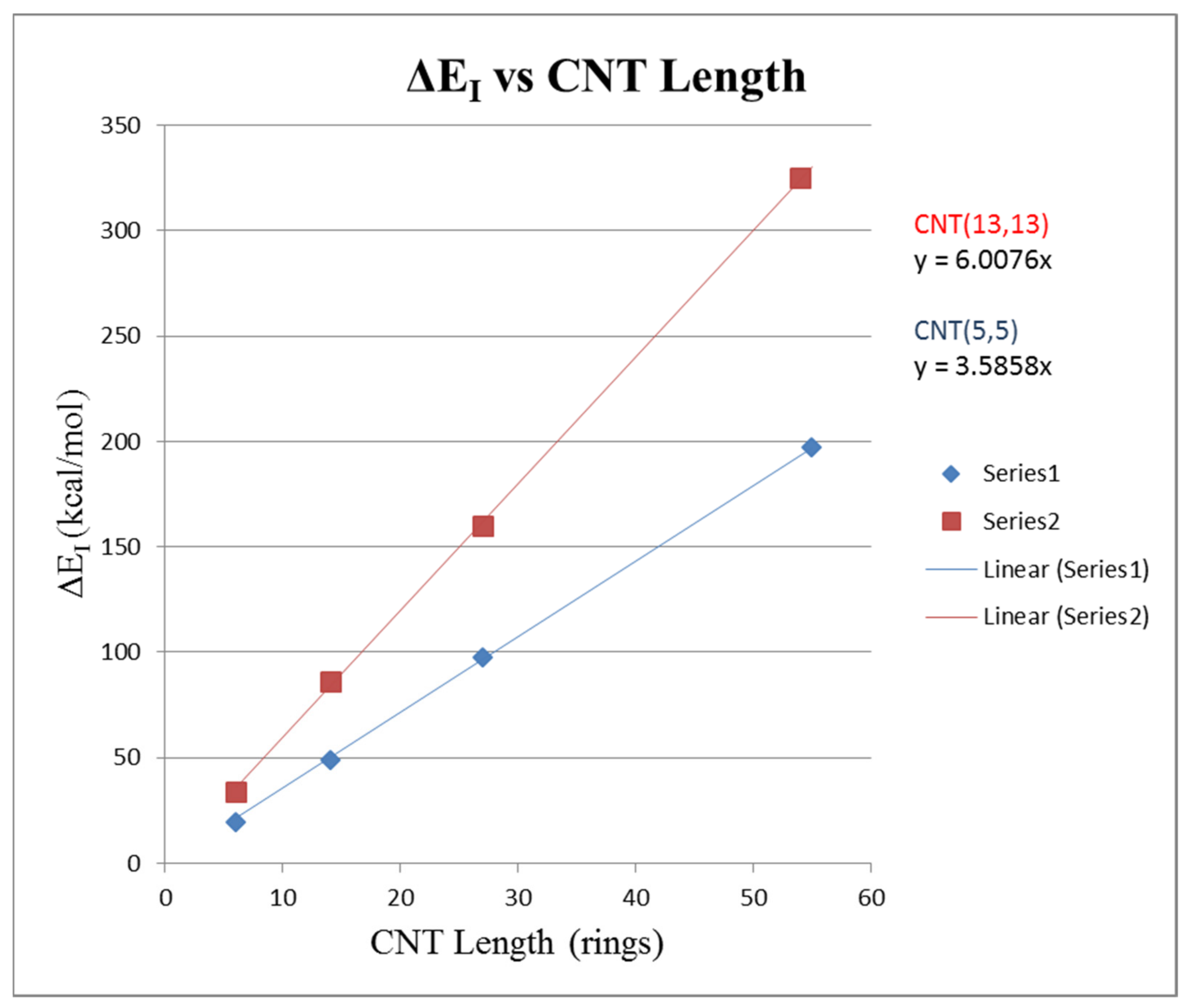
To consider the effect of length on a CNT–CNT interaction, the (5,5) CNT with a circumference of 5–phenyl rings and the CNT(13,13) with a circumference of 13–phenyl rings were used. The objective was to analyze how the change in pair interaction energy ∆E₁ varied with the length of the carbon nanotubes making the pair. For the circumference C_r = 5 CNTs, models of length Z_r = 6, 14, 27, and 55 were constructed. For the circumference C_r = 13 CNTs, models of lengths of Zr = 6, 14, 27, and 54 rings were constructed.

∆E₁ was calculated, as in prior work, by placing the two CNTs parallel and finding the energy when the two CNTs were separated and isolated and then subtracting from that value the total energy when the two CNTs were parallel and adjacent.

Table 2. Pair binding energy ∆E₁ (kcal/mol) as function of CNT circumference, C_r, in rings and length, Z_r, in rings.

Circumference	Length	∆E1
Cr (Rings)	Zr (Rings)	(kcal/mol)
5	6	19.7
5	14	49.0
5	27	97.4
5	55	197.4
13	6	34.2
13	14	85.9
13	27	160.3
13	54	325.1

shows the increase in the ∆E₁ interaction energy as the CNTs’ length is increased. Figure 8 shows a plot of ∆E₁ versus CNT length expressed in the Z_r rings. Linear regression gave for (5,5) CNT pair ∆E₁ = 3.586 Z_r with R² = 0.9999 and for the (13,13) CNT pair ∆E₁ = 6.008 Z_r with R² = 0.9999. This result is expected, as the interaction energy should be directly proportional to the length of the CNTs contacted with each other in the pair.

One way to consider length is the number of rings Z_r in an absolute sense but another convenient representation is to use one length as a reference point. For example, if ∆E₁ at Z_r = 14 given by ∆E₁(Z_r = 14) is chosen as a reference length then for any length Z_r the expectation is that ∆E₁ for that length, with appropriate C_r reference CNT, is simply given by the following:

∆E₁(Z_r) = (Zr/14) ∆E₁(Z_r = 14)

(45)

or if Zr = 54 was the reference point, then we have the following:

∆E₁(Zr) = (Zr/54) ∆E₁(Zr = 54)

(46)

From Table 2 where C_r = 13 and if Z_r = 6, 14, 27, 54 then Z_r/54 gives 0.1111, 0.2593, 0.5000, and 1.000, respectively. Using the ∆E₁(Z_r = 54, C_r = 13) value of 325.1 kcal/mol as a reference point then Equation (46) predicts for Z_r = 6, 14, and 27; ∆E₁ values of 36.1, 84.3, and 162.6 kcal/mol, respectively. For Z_r = 6, 14, 27; the values found directly from MM2 calculations in Table 2 are 34.2, 85.9, and 160.3 kcal/mol, respectively. The percent errors for the formula results relative to the MM2 calculation results are thus 5.6%, 1.9%, and 1.4%.

To solve the energy per interaction for a CNT with certain circumference (C_r) and length (Z_r) parameters, in general, a combination of Equations (43) and (45) gives the following:

ΔE₁ = (4.0277 C_r + 28.283) (Z_r/14)

(47)

or simply

ΔE₁ = 0.2877 C_r Zr + 2.020 Z_r

(48)

Any length could be chosen as a reference point and so Equation (48) merely provides one example of this approach. Thus, Equation (48) allows a quick estimate of the CNT pairwise binding energy given the values of C_r and Z_r.

Finally, the equation-based total bundle energy is given by the following:

ΔE(bundle) = I ∆E₁

(49)

where, as defined previously, I is the number of interactions in a bundle and ∆E₁ is the interaction energy for one CNT–CNT interaction.

4. Discussion

The dispersive interactions among CNTs were examined by ab initio theory calculations and by a van der Waals density functional theory (vdW-DFT) approach that was used to find the binding energies for a pair of nanotubes and a nanotube crystal [33]. The vdW-DFT results were consistent with interlayer binding in graphitic surfaces. It was observed that the nanotube crystal energy could be approximated by summation of nanotube pair interactions [33]. This observation supports our pairwise approach to the total binding energy within a CNT bundle. However, this pairwise approach becomes more problematic for very small CNTs.

The vdW analysis of nanotubes of widths greater than 5 nm and pairwise Lennard–Jones interactions showed the advantages of packing dislocations and the possibility of collapsed tubes to present larger vdW graphitic interfaces [34]. This work shows that our idealized situation likely is more appropriate for smaller, less flexible tubes. Moreover, it shows our packing arrangements as modeled are an idealized version of what is likely to be a more complicated and less perfect packing arrangement. In their computationally observed collapse of CNTs walls, a “dog bone” shape was observed with bulges at the ends. The flattened CNTs were able to achieve a stabilization due to greater surface area of adjacent tubes in mutual contact [34]. This again points to the practical limitations of our approach if CNTs are distorted from their ideal cylinder tube shape.

To get a sense of the structural strength of CNT bundles, a comparison with chemical bonds can be useful. For Zr = 27 and Cr = 5, the binding energy holding two (5,5) CNT together from our formula in Equation (48) is 97 kcal/mol. By comparison the C–H bond energy is about 99 kcal/mol and the C–C bond energy is about 83 kcal/mol. Thus, the vdW force, although considered weak, can be significant as the number of atoms in a molecular component are increased. Larger bundles, longer tubes, and larger-circumference tubes can enhance the total bundle-binding energy.

The formula to estimate CNT–CNT binding energies were based only on armchair CNTs and so could be modified for other CNT types although the vdW tube interactions may be similar. The CNTs examined here ranged from Cr of 4 to 15 and Z_r of 6 to 54. These limits extend to large-diameter tubes, where our approach is idealized on the assumption of no tube collapse or distortion. Our work is designed to point to possibilities of estimating total binding energies for a series of structural CNT bundles based on appropriate approximations. The appropriate range of stable CNTs would have to be considered, as well as appropriate parameters to model the interaction energy. Thus, our work is to demonstrate an approach that, where applicable, can save computational time by not having to recalculate for every possible nanostructure bundle of CNTs that may be of interest.

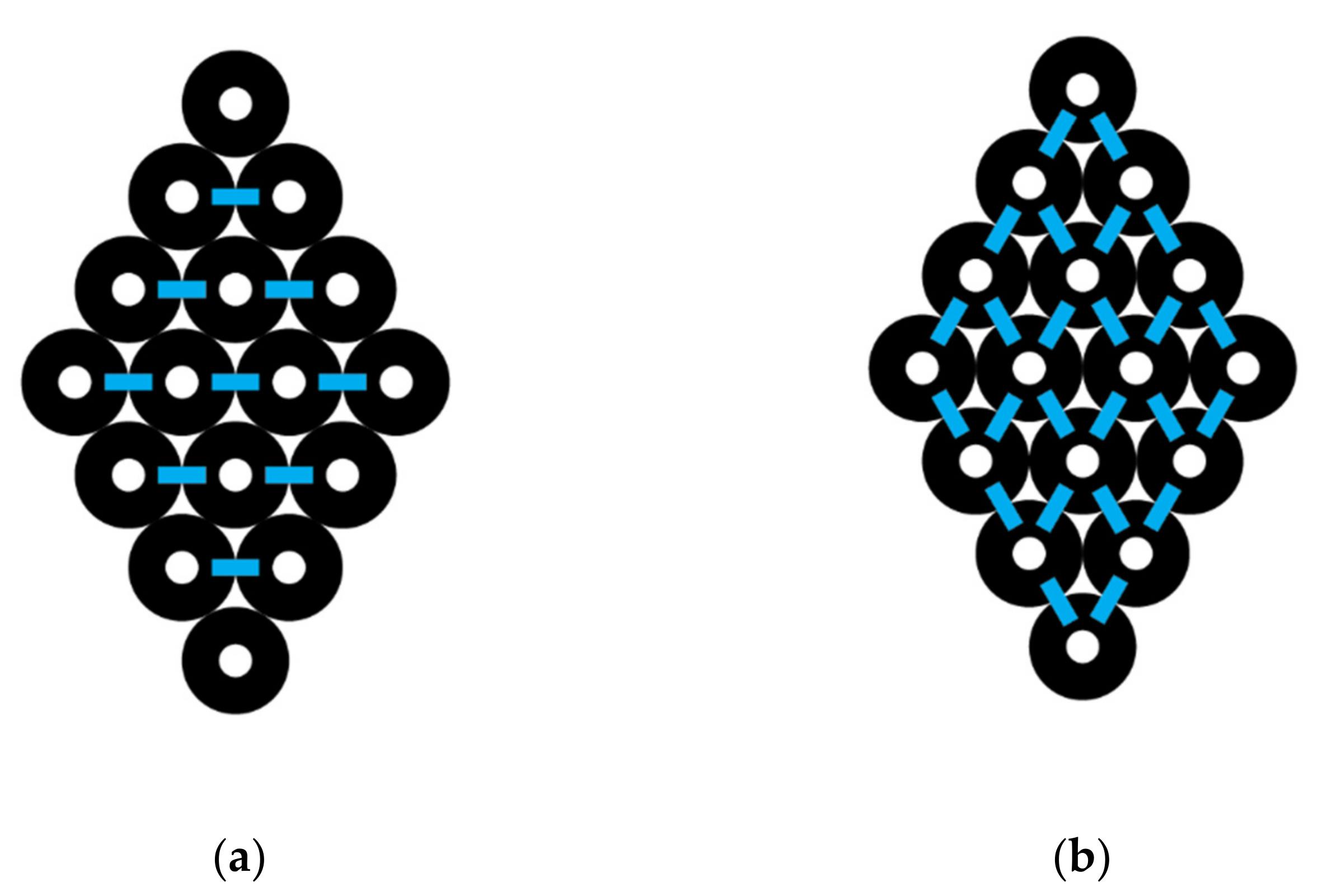
It should be noted that there is some redundancy built into the shape definitions and interaction formulas. For example, the hexagon shown in Figure 2 has 90 interactions based on I(hexagon) formula in Equation (21). However, this shape could also be considered a truncated diamond and the I(diamond) formula in Equation (13) applied. This equation would be based on a diamond shape where L is 3 and N₀ is 7. In this case, Equation (13) would give I(diamond) = 6(3)(7) – 3(3)² – 5(3) + 7 − 1 or 90 interactions. Thus, whichever definition most conveniently applies can be used.

Consider the smaller groups of four CNTs and two CNTs in Figure 2 in which the pairwise interactions can easily be counted as 5 and 1, respectively. Note that these small groups could be taken as extreme examples of the smallest diamond and truncated diamond shapes. For the four CNT group, N₀ = 2 and L = 1, and so Equation (13) gives 6(1)(2) − 3(1)² − 5(1) + 2 − 1 or 5, as expected. Furthermore, a simple pair of CNTs can be considered as a truncated diamond with no layers, so L = 0 and the central part of the “diamond shape” has two CNTs so N₀ = 2. Notice that, even in this extreme case, Equation (13) correctly give I(diamond) = 6(0)(2) − 3(0)² – 5(0) + 2 − 1 = 1, or a single pairwise interaction.

Two specific examples are considered for application of the equation approach by using Equation (48) to find ∆E for a bundle. These equation results are compared to the full molecular mechanics’ calculations based on Equation (41). The molecular mechanic MM2 force field result and then the equation result are given for each example below.

In the first example, a hexagon-shaped bundle of 7 CNTs was created with C_r = 13 and Z_r = 54. The model was required to represent 19,838 carbon atoms in the CNT bundle. MM2 calculations of an isolated CNT component and the seven CNT bundle gave from Equation (41) a calculation value of ∆E(bundle) = 3774 kcal/mol.

A hexagon-shaped bundle of seven CNTs has a single layer, so L = 1, and from Equation (21), the number of interactions based on L = 1 is I = 9L² + 3L or I = 12. Using Equation (48) and the values of C_r and Z_r gives the individual binding energy as ΔE₁ = 0.2877(13)(54) + 2.020(54) or ΔE_I = 311 kcal/mol. Because the total molecular mechanics analysis of isolated tubes and bundled tubes matches the pairwise summation, this agreement shows that anything beyond nearest neighbor makes a negligible contribution. This assumption becomes less appropriate only with extremely small CNTs.

The equation-based total bundle energy is given by Equation (49), where I is the number of interactions and ∆E₁ is the pairwise CNT–CNT interaction energy. For this example, where I = 12 and ΔE_I = 311 kcal/mol, we see that, from Equation (49), ΔE(bundle) is 3732 kcal/mol. This equation-based value of 3732 kcal/mol differs from the detailed molecular mechanics calculated value of 3774 kcal/mol by 1.1%.

In a second example, a hexagon-shaped bundle of 37 CNTs was created with C_r = 5 and Z_r = 12. The model required representing 9250 carbon atoms in the CNT bundle. MM2 calculations of the isolated CNT component and the 37 CNT bundle gave from Equation (41) a calculation value of ∆E(bundle) = 3625 kcal/mol.

A hexagon-shaped bundle of 37 CNTs has L = 3, and from Equation (21), the number of interactions based on L = 3 is I = 9L² + 3L or I = 90. Using Equation (48) and the values of C_r and Z_r gives ΔE₁ = 0.2877(5)(12) + 2.020 (12) or ΔE_I = 41.5 kcal/mol. The equation-based total bundle energy is given by Equation (49) and is therefore 90 times 41.5 kcal/mol, or 3735 kcal/mol. This equation-based total bundle energy value of 3735 kcal/mol differs from the MM2 calculated value of 3625 kcal/mol by 3.0%.

5. Conclusions

Formulas dependent on the shape and size of a bundle of aligned carbon nanotubes were derived to estimate the total binding energy for all the CNTs within a given bundle. The bundle shape and size determined the total number of pairwise interactions among the CNTs. For armchair type CNTs, the length and circumference of the component tubes were used to predict the strength of the pairwise interaction between two adjacent tubes. The noncovalent binding energy due to van der Waals forces associated with a single interaction between pairs of touching nanotubes was multiplied by the number of pairwise interactions to determine the total bundle binding energy (∆E). Force-field calculations were used to confirm the reliability of this bundle-formula approach. The formula results were compared to the binding energy found by taking the energy difference between the isolated component carbon nanotubes and the intact bundle.

In future work, the simple equations developed for the interactions within the bundle shapes of diamond, hexagon, parallelogram, and rectangle could be supplemented by other possible shapes and formulas. Moreover, a more general formal for other types of CNTs beside the armchair configuration could be used. In addition, the interaction binding energy of other repeated nanocomponents could be used in combination with these CNTs formulas to find the structural binding energy for possible mixed supramolecular structures.