Theoretical and Numerical Analysis of Nonlinear Processes in Amperometric Enzyme Electrodes with Cyclic Substrate Conversion

Abstract

A theoretical model of amperometric enzyme electrodes has been developed in which chemical amplification occurs in a single enzyme membrane via cyclic substrate conversion. The system is based on non-stationary diffusion equations with a nonlinear factor related to the Michaelis–Menten kinetics of the enzymatic reaction. By solving the nonlinear equations using the AGM technique, simple analytical expressions of concentration substrate, product, and amperometric current response are derived. Further, biosensor sensitivity, resistance, and gain are obtained from the current. MATLAB programming was used to carry out the digital simulation. The analytical results are validated with the numerical results. The effect of substrate concentration, maximum enzymatic rate, and membrane thickness on biosensor response was evaluated.

1. Introduction

Biosensors are two-component devices that consist of a biological entity, typically a redox enzyme that recognises the target analyte, and a transducer that converts the bio-recognition event between the biocatalyst and reactant/substrate (typically a binding/adduct formation process between the active site and substrate) into a measurable signal. Electrochemical or amperometric biosensors measure variations in a current at a working indicator electrode arising from the direct electrochemical oxidation or reduction of the biochemical reaction products [1,2,3,4,5,6,7,8,9]. Amperometric biosensors typically operate in a batch mode under conditions of constant applied electrode potential with concomitant monitoring of the steady-state current response arising from an electron transfer reaction at the sensor/electrode interface. This current is directly related to the concentration of the analyte. Amperometric biosensors are safe, inexpensive, and environmentally friendly, and, consequently, have found significant clinical and industrial applications.

It is very important to be able to quantitatively describe reaction and diffusion within bounded surface regions of the type encountered in amperometric biosensor systems. Typically, such systems may be very complex, and the challenge is to develop the simplest mathematical model that enables the description of the steady-state or transient current as a function of the substrate concentration. Typically, the mathematical model involves proposing a geometry-dependent reaction/diffusion equation subject to well-defined initial and boundary conditions for the substrate concentration within the bounded biosensing layer, which reflect the experimental conditions relevant to the sensing process. Typically, it is assumed that substrate transport is described by Fick’s law of diffusion and the reaction kinetics quantified in the first instance by the Michaelis–Menten rate equation. This is usually a good choice since Michaelis–Menten kinetics describe a binding event or adduct formation process that typifies the interaction between an immobilized enzymatic active site and a substrate molecule. Hence, using this approach, an approximate analytical solution to the boundary value problem describing the biosensor operation can be developed, which will describe the steady state or transient concentration profiles of reactant and product through the bound catalytic layer as a function of distance and time. It also enables an expression for the net reaction rate or flux expressed as a current to be derived. This can be related in a definite manner to real system parameters such as catalyst loading, catalyst concentration, substrate concentration, and layer thickness. The mathematical model should make simple predictions on how the reaction rate depends on each of the latter parameters and thereby enable the rational design of a modified electrode sensor in which substrate detection/catalysis is optimized.

The sensitivity of an amperometric sensor is a useful parameter and determines the detection limit of the device. Recently, Rajendran and et al. derived analytical expressions for the current, sensitivity, and resistance of an amperometric biosensor operating where substrate inhibition [10], product inhibition [11], and uncompetitive inhibition processes [12] pertain. Furthermore, Joy Salomi et al. [13] have described the theoretical study of biosensor devices acting in a trigger mode. Analytical steady-state expressions describing the substrate and product concentrations within a bound enzyme thin film on an electrode surface for both non-Michaelis–Menten kinetics [14] and Michaelis–Menten kinetics [15] in an amperometric biosensor have also been derived by solving the pertinent nonlinear reaction/diffusion equations. The theoretical analysis for various types of complex biosensor systems has also been discussed [16,17,18].

The cyclic conversion of the substrate can enhance the sensitivity of the amperometric enzyme electrodes [19,20,21]. A membrane containing two enzymes is commonly used to execute the cyclic conversion of the substrate and analyte regeneration. The steady-state response of enzyme electrodes with cyclic substrates conversion was computed when first-order substrate kinetics pertain [19]. By solving diffusion equations and employing Green’s functions, the dynamic behaviour of these electrodes was investigated [22]. Other amperometric electrodes have been developed by utilising cyclic substrate conversion in single enzyme membranes [22]. In these electrodes, cyclic conversion of the substrate was carried out by conjugating the enzymatic reaction with the chemical or electrochemical process. The digital simulation of the biosensor response was carried out using the implicit finite difference scheme by various researchers [23,24,25].

This study aims to develop a simple theoretical model that allows the simulation of enzymatic biosensor responses using amplification through coupled electrochemical and enzymatic substrate conversion. The model created is based on non-stationary diffusion equations with a nonlinear factor related to the enzymatic reaction. These equations are analytically solved using the AGM technique. The MATLAB programme was used to perform the digital simulation of the biosensor responses, and this is used to check the accuracy of the analytical solution. The developed theoretical model was employed to investigate the influence of the substrate concentration and the maximal enzymatic rate, as well as the membrane thickness on the biosensor response, sensitivity, resistance, and amplification.

2. Mathematical Formulation of the Problem

The biosensor may be considered as an enzyme electrode consisting of a thin film membrane of thickness d containing an immobilised enzyme applied onto the surface of the electrochemical transducer. Consider the very simple scheme of a substrate S electrochemically converted to a product P at the surface of the support electrode. This product is then enzymatically transformed back to substrate S using an enzyme catalyst E. This is perhaps the most simple scheme for substrate cyclic conversion.

$$S\to P\stackrel{E}{\to }S$$

(1)

In the case of phenol-sensitive biosensors, for example, 1,2-benzoquinone (S) is reduced electrochemically and the product pyrocatechol (P) formed is then subsequently oxidised in the membrane using immobilised laccase as the enzyme catalyst (E). Coupling of the enzyme-catalysed reaction in the enzyme layer with planar diffusion, described by Fick’s law, leads to the following steady-state reaction/diffusion equations [26]:

For $0<x<d,$

$$D_S\frac{d^{2}S\left(x\right)}{d{x}^2}+\frac{V_{max}P\left(x\right)}{K_M+P\left(x\right)}=0$$

(2)

$$D_P\frac{d^{2}P\left(x\right)}{d{x}^2}-\frac{V_{max}P\left(x\right)}{K_M+P\left(x\right)} = 0$$

(3)

where $x$ stand for the distance coordinate and $S\left(x\right)$ and $P\left(x\right)$ denote the concentration functions of the substrate and reaction product, respectively. Note that $V_{max}$ is the maximal enzymatic rate attainable with that amount of enzyme when the enzyme is fully saturated with substrate. This is given by $V_{max}=k_{cat}{e}_{\Sigma }$, where k_cat denotes the catalytic rate constant and e_Σ denotes the total enzyme concentration in the layer. Note that $K_M$ denotes the Michaelis constant, $d$ the thickness of the enzyme layer, and $D_S$ and $D_P$ the diffusion coefficients of the substrate and product, respectively. Let $x=0$ represent the electrode surface, while $x=d$ represents the bulk solution/membrane interface. The operation of the biosensor begins when some substrate appears over the surface of the enzyme layer.

The electrode potential is chosen to ensure complete transformation of substrate to product at the electrode so that the substrate concentration at the electrode surface is zero. During electrochemical conversion, the product is produced. The rate of the product generation at the electrode is proportional to the rate of conversion of the substrate. When the solution is well-stirred outside the membrane, the diffusion layer ($0<x<d$) remains at a constant thickness. Consequently, the concentration of substrate, as well as product, over the enzyme surface (bulk solution/membrane interface) remains constant while the biosensor contacts the substrate solution. This is reflected in the boundary conditions given by:

$$S\left(x=0\right)=0$$

(4)

$$S\left(x=d\right)=S_0$$

(5)

$$D_S{\frac{dS}{dx}|}_{x=0}+D_P{\frac{dP}{dx}|}_{x=0}=0$$

(6)

$$P\left(x=d\right)=0$$

(7)

where $S_0$ is the concentration of substrate in the bulk solution. Note that we have neglected concentration polarization in the solution phase adjacent to the immobilized enzyme layer. This can, of course, be readily accounted for in the analysis.

The current is measured at the support electrode/enzyme layer interface and defines the response of the biosensor device to the chemical activity in the enzyme layer. The current depends upon the flux of the substrate $S$ at the electrode surface, i.e., at $x=0$. Consequently, the current density i can be obtained explicitly from Faraday’s law and Fick’s law via:

$$i=n_{e}F{D}_S{\frac{dS\left(x\right)}{dx}|}_{x=0}=-n_{e}F{D}_S{\frac{dP\left(x\right)}{dx}|}_{x=0}$$

(8)

where $n_e$ is a number of electrons involved in a charge transfer at the electrode surface and $F$ is Faraday constant $F\approx 9.65\times {10}^4\mathrm{C}/\mathrm{mol}$.

Dimensionless Form of Problem

To facilitate further analysis, it is often useful to cast the reaction/diffusion problem into dimensionless form. We can make the reasonable assumption that $D_S=D_P=D.$ The dimensionless steady-state model of the system under consideration can be obtained from Equations (2) and (3) and is given as follows:

$$\frac{d^{2}u\left(X\right)}{d{X}^2}+\frac{{\sigma }^{2}v\left(X\right)}{1+\alpha v\left(X\right)}=0$$

(9)

$$\frac{d^{2}v\left(X\right)}{d{X}^2}-\frac{{\sigma }^{2}v\left(X\right)}{1+\alpha v\left(X\right)}=0$$

(10)

where the dimensionless variables are given by

$$u=\frac{S}{S_0}, v=\frac{P}{S_0} , X=\frac{x}{d} , {\sigma }^2=\frac{V_{max}{d}^2}{D K_M} , \alpha =\frac{S_0}{K_M}$$

(11)

The boundary conditions are transformed as follows:

$$\mathrm{At}X=0:u\left(X\right)=0, \frac{du\left(X\right)}{dX}+(\frac{dv\left(X\right)}{\partial X})=0$$

(12)

$$\mathrm{At}X=1:u\left(X\right)=1,v\left(X\right)=0$$

(13)

The current density in dimensionless form is [17]

$$\psi =\frac{i}{n_{\mathrm{e}}FD}\left[\frac{d}{S_0}\right]={\frac{du\left(X\right)}{dX}|}_{X=0}=-{\frac{dv\left(X\right)}{dX}|}_{X=0}$$

(14)

The steady-state current I of the biosensor is expressed as follows:

$$I=-\frac{n_{\mathrm{e}}FD{S}_0}{d}{\frac{dv\left(X\right)}{dX}|}_{X=0}$$

(15)

We note that the reaction/diffusion expressions presented in Equations (9) and (10) are nonlinear. Previously, such nonlinear equations were solved in the limit of low and high substrate concentrations. In this work we will proceed to use a recently established protocol to derive a useful analytical solution to these expressions which is valid over a wide region of substrate concentration.

3. An Approximate Analytical Expression of Steady-State Concentrations Using AGM

Recently, some nonlinear differential equations have been solved using several analytical or semi-analytical methods, even with strong nonlinearities. Of these methods, we mention the homotopy analysis method [27], the Adomian decomposition method [28], the variational iteration method [29], and the Green’s function iterative method [30,31]. Recently, the homotopy perturbation method (HPM) [32,33,34], the Akbari-Ganji method (AGM) [35,36,37], and the Taylor series method [38,39,40,41] have proven to be particularly useful and, therefore, have received a great deal of attention.

The approximate analytical expression for the dimensionless stationary concentration of substrate $u$ and product $v$ is obtained as follows (Appendix A):

$$u\left(X\right)=1-\mathit{cosh}\left(\sqrt{\gamma }X\right)+sinh\left(\sqrt{\gamma }X\right)coth\left(\sqrt{\gamma }\right)$$

(16)

$$v\left(X\right)=\mathit{cosh}\left(\sqrt{\gamma }X\right)-sinh\left(\sqrt{\gamma }X\right)coth\left(\sqrt{\gamma }\right)$$

(17)

where we note that:

$$\gamma =\frac{{\sigma }^2}{1+\alpha }$$

(18)

We can also show that the normalised current becomes:

$$\psi =\sqrt{\gamma }coth\left(\sqrt{\gamma }\right)$$

(19)

The steady-state current I is given by

$$I=\frac{n_{e}FD{S}_0}{d}\sqrt{\gamma }coth\left(\sqrt{\gamma }\right)$$

(20)

This general expression for the steady-state current response is valid over a wide range of substrate concentrations. We now examine some interesting limiting cases corresponding to the situation where the concentration of substrate is much less than the Michaelis constant and when it is much greater.

3.1. Limiting Case: Unsaturated (First-Order) Catalytic Kinetics

We first consider the situation where the substrate concentration level in the enzyme layer is less than the Michaelis constant $K_M$, ($S_0$ << $K_M$). This situation will pertain when $av\ll 1$. In such circumstances, Equations (8) and (9) reduce to the linear reaction–diffusion equations:

$$\frac{d^{2}u\left(X\right)}{d{X}^2}+{\sigma }^{2}v\left(X\right)=0$$

(21)

$$\frac{d^{2}v\left(X\right)}{d{X}^2}-{\sigma }^{2}v\left(X\right)=0$$

(22)

By solving Equations (21) and (22) with their corresponding boundary conditions (Equations (12) and (13)), the exact expression of the concentrations of substrate $u$ and product $v$ and current has been obtained as follows:

$$u\left(X\right)=1-cosh\left(\sigma X\right)+coth\left(\sigma \right)sinh\left(\sigma X\right)$$

(23)

and

$$v\left(X\right)=cosh\left(\sigma X\right)-coth\left(\sigma \right)sinh\left(\sigma X\right)$$

(24)

The steady-state current I is

$$I=\frac{n_{\mathrm{e}}FD{S}_0}{d}\sigma coth\left(\sigma \right)$$

(25)

This expression is valid for all values of the parameter σ.

3.2. Limiting Case: Saturated (Zero-Order) Catalytic Kinetics

We now examine the situation where the substrate concentration level in the enzyme layer is greater than the Michaelis constant $K_M$, ($S_0$ >> $K_M$). This situation will pertain when $av\gg 1$. Here, Equations (9) and (10) reduce to the linear reaction–diffusion equations:

$$\frac{d^{2}u\left(X\right)}{d{X}^2}+\frac{{\sigma }^2}{\alpha }=0$$

(26)

$$\frac{d^{2}v\left(X\right)}{d{X}^2}-\frac{{\sigma }^2}{\alpha }=0$$

(27)

By solving Equations (26) and (27) with their corresponding boundary conditions (Equations (12) and (13)), the exact expression of the concentrations of substrate $u$ and product $v$ and current has been obtained as follows:

$$u\left(X\right)=\left(1+\frac{{\sigma }^2}{2\alpha }\right)X-\frac{{\sigma }^2}{2\alpha }{X}^2$$

(28)

and

$$v\left(X\right)=1-\left(1+\frac{{\sigma }^2}{2\alpha }\right)X+\frac{{\sigma }^2}{2\alpha }{X}^2$$

(29)

The steady-state current I is

$$I=\frac{n_{\mathrm{e}}FD{S}_0}{d}\left(1+\frac{ {\sigma }^2}{2\alpha }\right)=\frac{n_{e}FD{S}_0}{d}+\frac{n_{e}F{k}_{cat}{e}_{\mathsf{\Sigma }}d}{2}$$

(30)

We note that the latter expression contains two terms. The first corresponds to the diffusion of substrate through the matrix. The second corresponds to the decomposition of the product/enzyme complex to regenerate the substrate. The factor of 2 arises from the fact that the product generated at the electrode may also be lost by diffusion through the enzyme layer, as well as reacting at the enzyme to generate substrate S. Here, the product concentration is much larger than the Michaelis constant of the enzyme (p/K_M >> 1).

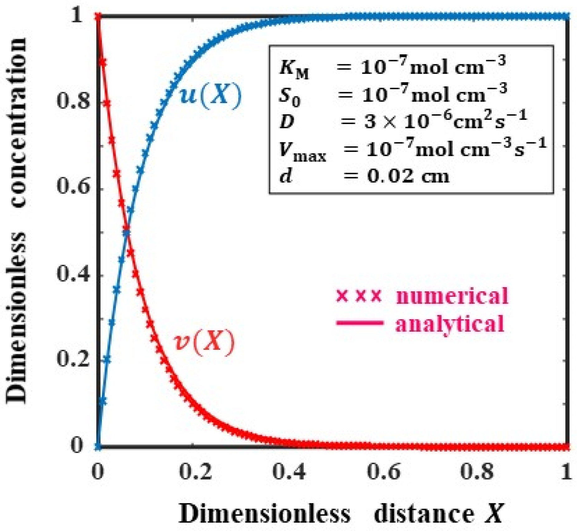
4. Validation of Analytical Results

In this section, we present numerical simulations to test the accuracy and reliability of the proposed method. The analytical expressions obtained in this paper have been compared with the highly accurate numerical solution obtained by the MATLAB routine bvp4c, which is a finite-difference code that implements the three-stage Lobatto IIIA formula. The analytically derived (Equations (16) and (17)) and computationally simulated concentration profiles of substrate and product within the enzyme layer are compared in Figure 1. These curves were computed for the following typical parameter values: K_M = 10⁻⁷ mol cm⁻³, S₀ = 10⁻⁷ mol cm⁻³, D = 3 × 10⁻⁶ cm² s−¹, d = 0.02 cm, and V_max = 10⁻⁷ mol cm⁻² s⁻¹. The analytical and numerical solutions were plotted on the same coordinates for a wide range of possible values of the underlined problem parameters. It is clear from

Table 1. Comparison of dimensionless concentration of the substrate S and product $P$ with simulation results for the parameter values $D=3\times \frac{{10}^{-6}{\mathrm{cm}}^2}{\mathrm{s}}, V_{max}=\frac{{10}^{-8}\mathrm{mol}}{{\mathrm{cm}}^3\mathrm{s}}, K_M=\frac{{10}^{-7}\mathrm{mol}}{{\mathrm{cm}}^3},S_0=\frac{{10}^{-8}\mathrm{mol}}{{\mathrm{cm}}^3},\mathrm{and}d=0.02\mathrm{cm}$.

X	Concentration of the Substrate S			Concentration of the Product P
	Numerical	AGM Equation (16)	% of Deviation	Numerical	AGM Equation (17)	% of Deviation
0	0	0	0	1	1	0
0.1	0.1326	0.1317	0.68	0.8674	0.8683	0.10
0.2	0.2545	0.2528	0.67	0.7455	0.7472	0.23
0.3	0.3672	0.3649	0.63	0.6328	0.6351	0.36
0.4	0.4719	0.4693	0.55	0.5281	0.5307	0.49
0.5	0.5699	0.5672	0.47	0.4301	0.4328	0.63
0.6	0.6624	0.6599	0.38	0.3376	0.3401	0.74
0.7	0.7506	0.7485	0.28	0.2494	0.2515	0.84
0.8	0.8355	0.8340	0.18	0.1645	0.1660	0.91
0.9	0.9183	0.9175	0.09	0.0817	0.0825	0.98
1	1	1	0	0	0	0
	Average deviation		0.36	Average deviation		0.02

that the fit between the analytical solution to the reaction/diffusion problem in the form of reactant and product concentration profiles, and the corresponding quantity numerically evaluated using MATLAB, is excellent, with average deviation between numerical and analytical results being typically 0.36% for substrate and 0.02% for product.

5. Results and Discussion

We note that the solution of the nonlinear reaction/diffusion equations as expressed in Equations (16) and (17) represents new and simple analytical expressions for the concentration substrate and product, respectively. Furthermore, the amperometric current response is described by Equation (20) for all parameter values.

5.1. Influence of Parameter on Concentration of Substrate and Product

The dimensionless concentration profiles of substrate u and product v involved in the cyclic substrate conversion following Michaelis–Menten kinetics are depicted in Figure 1. The experimental values of the parameters used in this figure are K_M = 10⁻⁷ mol cm⁻³, S₀ = 10⁻⁷ mol cm⁻³, D = 3 × 10⁻⁶ cm² s−¹, d = 0.02 cm, and V_max = 10⁻⁷ mol cm⁻² s⁻¹ [26]. From the figure, it can be noted that our obtained analytical result matches quite well with the numerical experiments. Peculiarities of the biosensor activity have been examined using our analytical result for various values of the parameters. The nonlinear distribution of concentration of both compounds throughout the membrane can be observed, and it is noted that the substrate concentration $u$ decreases and the product concentration $v$ increases significantly with decrease of dimensionless distance $X$ from the outer edge of the membrane to the inner electrode/film interface.

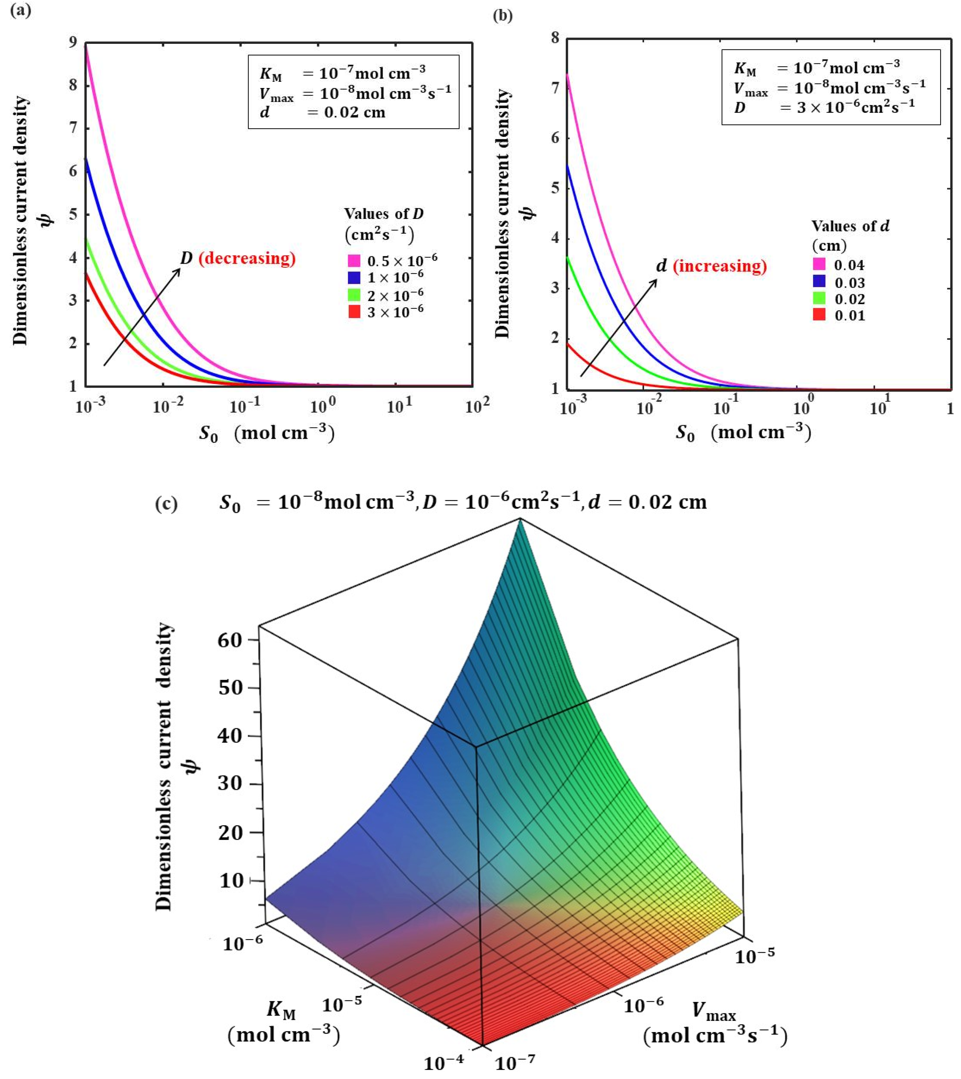
5.2. Influence of Transport and Reaction Parameters on the Current Response

In Figure 2$\mathrm{a}$,$\mathrm{b}$ the dependence of the maximal biosensor current $\psi$ on the substrate concentration $S_0$ for various values of diffusion coefficient $D$ and the thickness of the enzyme layer $d$ is outlined. We note that the steady-state current response is a monotonously decreasing function of $S_0$ for all values of $D$ and $d.$ From Figure 3, it is noted that the biosensor current rises as $V_{\mathit{max}}$ increases and $K_M$ decreases. Further, it can be deduced that $S_0>1 {\mathrm{mol}\mathrm{cm}}^{-3}$ and the biosensor current is independent of the bulk substrate concentration$S_0$. This is to be expected since, under these conditions, the enzyme sites in the matrix are saturated with substrate.

5.3. Sensitivity of Biosensor

The term sensitivity refers to the change of the biosensor response with regard to a change in the substrate concentration. Since both the current and the substrate concentration vary in order of magnitude, dimensionless sensitivity is another valuable parameter to be considered. The mathematical representation of the non-dimensional biosensor sensitivity for substrate concentration $S_0$ can be estimated from the following [42]:

$$B_{\mathrm{s}}\left(S_0\right)=\frac{\partial I\left(S_0\right)}{\partial S_0}\times \frac{S_0}{I\left(S_0\right)}$$

(31)

where $B_s$ is biosensor sensitivity and$I\left(S_0\right)$ is steady-state current density measured at the substrate concentration $S_0$. Therefore, from Equation (20), we can readily show that:

$$B_{\mathrm{s}}\left(S_0\right)=\frac{\alpha }{\left(\alpha +1\right)}\left[\frac{1}{2}-\frac{\sqrt{\gamma }}{\mathit{sinh}\left(2\sqrt{\gamma }\right)}\right]$$

(32)

where $\alpha ,\gamma$ are defined in Equations (11) and (18). As the maximal enzymatic rate drops down, i.e., $V_{max}\to 0,$ it can be observed that $B_{\mathrm{s}}$ also tends to zero. Quick diffusivity contributes to relatively low sensitivity. Figure 3a supports this inference. When the membrane thickness and enzymatic rate vary by two orders of magnitude, a similar effect is again observed. This shows that thickness of the membrane plays a crucial role in determining the biosensor sensitivity and Figure 3b confirms the same. It is possible to observe from the smooth curves of Figure 3a,b that $0\le B_{\mathrm{s}}\le 0.5$ for all values of the parameters. This assertion receives further confirmation in the 3D plot as outlined in Figure 3c.

Figure 3. (a) Variation of biosensor sensitivity as a function of bulk substrate concentration for various values of diffusion coefficient. (b) Variation of biosensor sensitivity with substrate concentration for different values of enzyme layer thickness. (c) Three-dimensional representation of the variation of biosensor sensitivity with both maximum enzymatic reaction rate and Michaelis constant value.

Figure 3. (a) Variation of biosensor sensitivity as a function of bulk substrate concentration for various values of diffusion coefficient. (b) Variation of biosensor sensitivity with substrate concentration for different values of enzyme layer thickness. (c) Three-dimensional representation of the variation of biosensor sensitivity with both maximum enzymatic reaction rate and Michaelis constant value.

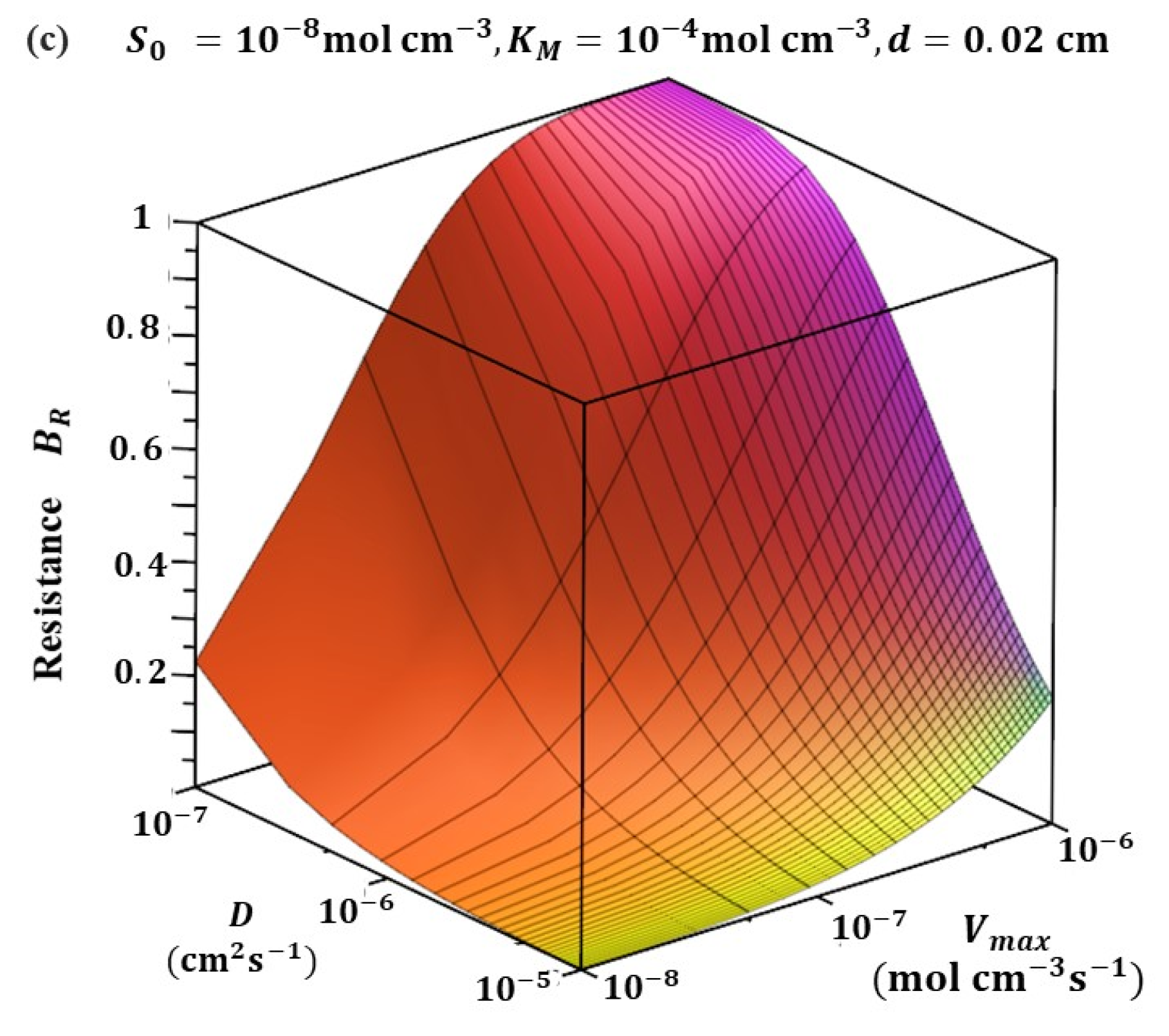
5.4. Resistance of Biosensor

The normalised resistance $B_{\mathrm{R}}$ is represented as the gradient of steady-state biosensor current concerning the thickness of membrane $d$ [42]:

$$B_{\mathrm{R}}\left(d\right)=\frac{\partial I\left(d\right)}{\partial d}\times \frac{d}{I\left(d\right)}$$

(33)

where $I$ is the steady-state current density measured at membrane thickness $d$. From Equation (32) we obtain

$$B_{\mathrm{R}}\left(d\right)=1-\frac{2\sqrt{\gamma }}{\mathit{sinh}\left(2\sqrt{\gamma }\right)}$$

(34)

From the Equations (32) and (33), the new relationship between sensitivity and resistance can be shown as $B_{\mathrm{s}}\left(S_0\right)=\frac{\alpha }{2\left(\alpha +1\right)}{B}_{\mathrm{R}}\left(d\right)$. Hence, there is almost zero resistance for negligibly small values of $V_{\mathit{max}}$. This can also be observed in the three-dimensional representation of $B_{\mathrm{R}}$ as a function of transport and enzyme kinetics, as presented in Figure 4c. Moreover, from the latter curve we note that the biosensor resistance increases as the diffusion coefficient decreases. The range of biosensor resistance as depicted by the nonlinear curves of Figure 4a,b lies within the bounds from 0 to 1 for all values of the parameters. Both $K_M$ and $S_0$ have a similar effect in the sense that, for their lower values, the device resistance increases.

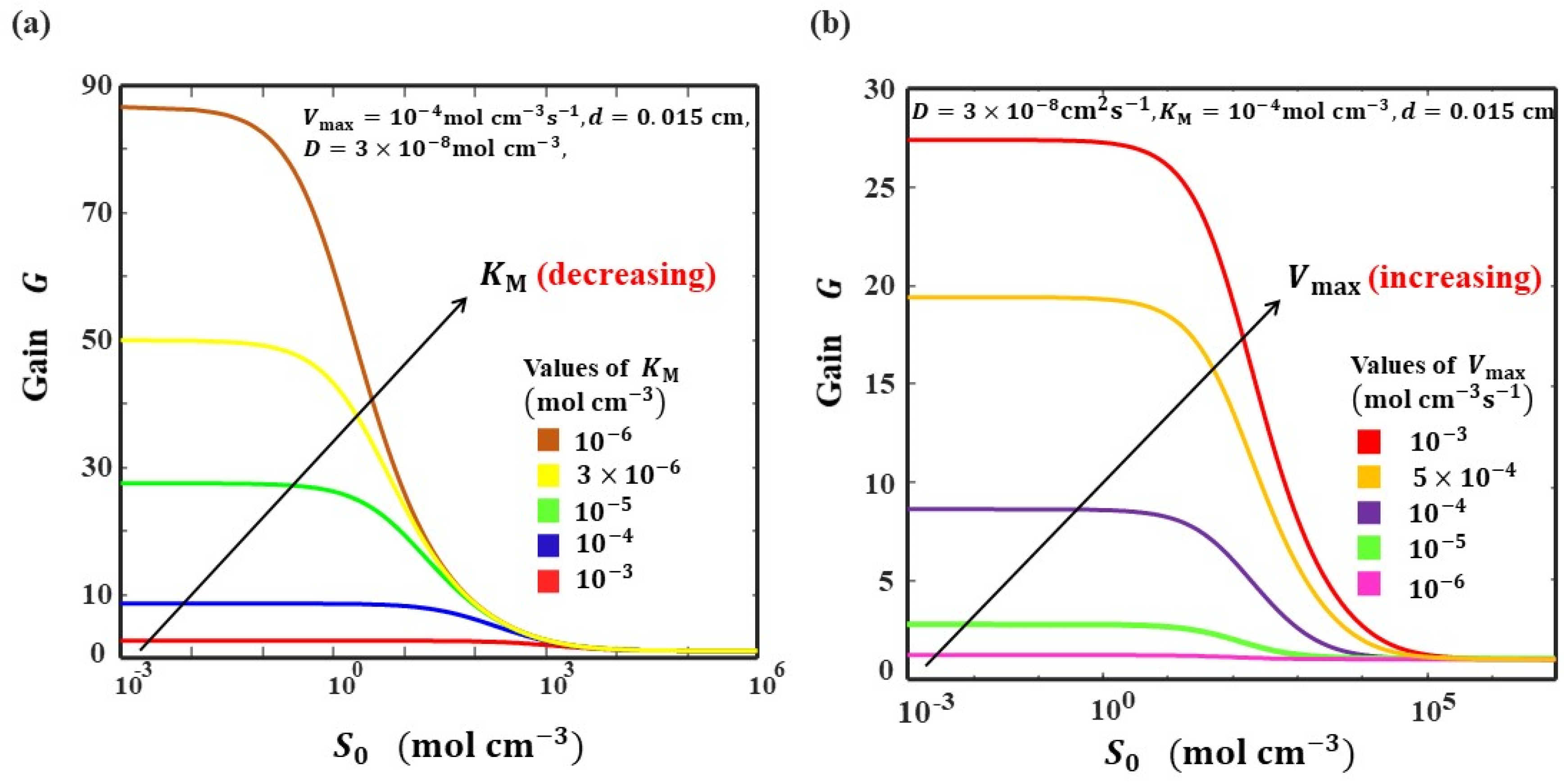
5.5. Gain of the Biosensor

Sensitivity gain is described as the ratio of the trigger biosensor’s steady-state current ($I_{\mathrm{CEC}}$) to the corresponding CE biosensor’s steady-state current ($I_{\mathrm{CE}}$). This is used to compare the amplified and non-amplified biosensor response. Now, if the enzyme is absent and substrate recycling is absent, then the applied potential dictates that the device is operating under mass transport control, a steady-state limiting current is observed, and the normalised current density is given by $\psi ={\psi }_L=1$. Then, the amplification, or gain factor G, can be defined by:

$$G\left(V_{\mathit{max}}\right)=\frac{I\left(V_{\mathit{max}}\right)}{I\left(V_{\mathit{max}}=0\right)}=\sqrt{\gamma }coth\left(\sqrt{\gamma }\right)$$

(35)

We note that the gain factor $\psi /{\psi }_L=\sqrt{\gamma }\mathit{coth}\left(\sqrt{\gamma }\right)$ depends on the Michaelis–Menten parameters associated with the enzyme catalysis P → S reaction. When $\sqrt{\gamma }<<1$, we note that $\mathit{cot}h\left(\sqrt{\gamma }\right)\cong \frac{1}{\sqrt{\gamma }}\left\{1+\frac{\gamma }{3}\right\}$, and so the gain factor is given by:

$$G\cong 1+\frac{\gamma }{3}$$

(36)

In contrast, when $\sqrt{\gamma }\gg 1$, then $\mathit{cot}h\left(\sqrt{\gamma }\right)\cong 1$ and the gain factor is given by:

$$G\cong \sqrt{\gamma }$$

(37)

These expressions are valid for all values of the saturation parameter $\alpha$.

Figure 5 displays the dependence of the gain $G$ of the steady-state current on the substrate concentration $S_0$ for thinner biosensor film thicknesses $d$. The gain increases up to 27 times approximately at $S_0>1 {\mathrm{mol}\mathrm{cm}}^{-3}$ and $V_{\mathit{max}}={10}^{-3}{\mathrm{mol}\mathrm{cm}}^{-3}{\mathrm{s}}^{-1}.$ For $V_{\mathit{max}}\le {10}^{-6}{\mathrm{mol}\mathrm{cm}}^{-3}{\mathrm{s}}^{-1}$, the gain is less than 4 and is linear, whereas for $K_M\le {10}^{-3}{\mathrm{mol}\mathrm{cm}}^{-3},$the gain is the linear function of $S_0$.

We now mention a subtle but important point [43]. We need to evaluate the relationship between the observed flux, which is manifested as a current flow arising from the heterogeneous electrochemical reaction of the substrate S at the electrode surface, and the reaction flux corresponding to the formation of substrate S formed via reaction of the product species P at the enzyme surface. As shown in Appendix B, the observed flux giving rise to the experimentally measured current is related to the substrate regeneration flux f_S at the enzyme in the diffusion layer via

$$f_{obs}=\frac{1+\mathsf{\Phi }/2}{1+\mathsf{\Phi }}{f}_S=\eta f_{S }$$

(38)

Here, we have introduced an efficiency factor η which determines how much substrate regenerated by the enzymatic reaction of P is lost to the solution and which cannot take place in amplification. We note that the efficiency factor takes the following form:

$$\eta =\frac{1+\mathsf{\Phi }/2}{1+\mathsf{\Phi }}$$

(39)

This function is presented in Figure A1 in Appendix B. When Φ = 1, then η = 0.75. Hence, under these circumstances, 25% of the substrate regenerated via the reaction of the product P with the enzyme E is lost via diffusion to the bulk solution and cannot participate in the electrochemical reaction at the electrode surface, and hence in signal amplification.

6. Analysis of ‘Mixed Case’ Moving Boundary Scenario Corresponding to Varying Levels of Saturation across the Enzyme Membrane

We have examined the limiting situations for totally saturated kinetics when $av\gg 1$ and unsaturated kinetics when $av\ll 1.$ We can also envisage the more complex situation where the level of saturation varies across the thickness of the enzyme film [44]. The simplest strategy involves the assumption that the inner part of the film is unsaturated, while the outer region of the film remains saturated. A moving normalized distance parameter $X^{*}$ located between the two regions under consideration can be introduced. As the substrate $P$ diffuses into the film, a reaction front will have been established at $X=X^{*}.$ When $X^{*}=1,$ the entire region is unsaturated, while at$X^{*}=0$, the entire region is saturated. Now, at $=X^{*},$ $v=\frac{1}{\alpha }$. Hence, Equation (17) becomes

$$\frac{1}{\alpha }=\mathit{cosh}\left(\sqrt{\gamma }{X}^{*}\right)-sinh\left(\sqrt{\gamma }{X}^{*}\right)coth\left(\sqrt{\gamma }\right)$$

(40)

On solving the above Equation (40), $X^{*}$ can be obtained as follows:

$$X^{*}=\frac{1}{\sqrt{\gamma }}\left[ln\left(-\frac{1}{2\alpha }\left(exp{\left(\sqrt{\gamma }\right)}^2-1-\sqrt{{\left(exp{\left(\sqrt{\gamma }\right)}^2-1\right)}^2+4{\alpha }^{2}exp{\left(\sqrt{\gamma }\right)}^2}\right)\right)\right]$$

(41)

This expression indicates the manner in which the location of the moving boundary varies with the kinetic parameter γ and the saturation parameter α.

7. Conclusions

In this paper, we have shown that a simple mathematical model of an amperometric biosensor operation can be successfully used to investigate and predict the dynamics of the response of the device when a cyclic substrate conversion operates. New and simple approximate analytical expressions of substrate and product concentrations, steady-state current, sensitivity, and biosensor resistance are reported. The effect of various physical parameters, such as membrane thickness, Michaelis constant, and maximum catalytic rate on the latter key performance indicators, is also discussed. This theoretical result can be applied in designing novel, highly sensitive biosensors, which minimise enzyme volume without losing sensitivity.

References

1. Crank, J. The Mathematics of Diffusion, 2nd ed.; Clarendon Press: Oxford, UK, 1975. [Google Scholar]
2. Clark, L.C.; Lyons, C. Electrode system for continuous monitoring in cardiovascular surgery. Ann. N. Y. Acad. Sci. 1962, 102, 29–45. [Google Scholar] [CrossRef]
3. Turner, A.P.F.; Karube, I.; Wilson, G.S. Biosensors: Fundamentals and Applications; Oxford University Press: Oxford, UK, 1987. [Google Scholar]
4. Rogers, K.R. Biosensors for environmental applications. Biosens. Bioelectron 1995, 10, 533–541. [Google Scholar] [CrossRef]
5. Wollenberger, U.; Lisdat, F.; Scheller, F.W. Frontiers in Biosensorics 2, Practical Applications; Birkhauser Verlag: Basel, Switzerland, 1997. [Google Scholar]
6. Chaubey, A.; Malhotra, B.D. Mediated biosensors. Biosens. Bioelectron. 2002, 17, 441–456. [Google Scholar] [CrossRef]
7. Blaedel, W.J.; Boguslaski, R.C. Chemical amplification in analysis: A review. Anal. Chem. 1978, 50, 1026–1032. [Google Scholar] [CrossRef]
8. Fuhrmann, B.; Spohn, U. An enzymatic amplification flow injection analysis (FIA) system for the sensitive determination of phenol. Biosens. Bioelectron. 1998, 13, 895–902. [Google Scholar] [CrossRef]
9. Korotcenkov, G. Chemical Sensors: Simulation and Modeling; Electrochemical Sensors; Momentum Press: New York, NY, USA, 2013; Volume 5. [Google Scholar]
10. Swaminathan, R.; Devi, M.C.; Rajendran, L.; Venugopal, K. Sensitivity and resistance of amperometric biosensors in substrate inhibition processes. J. Electroanal. Chem. 2021, 895, 115527. [Google Scholar] [CrossRef]
11. Rani, R.U.; Rajendran, L.; Lyons, M.E.G. Steady-state current in product inhibition kinetics in an amperometric biosensor: Adomian decomposition and Taylor series method. J. Electroanal. Chem. 2021, 886, 115103. [Google Scholar] [CrossRef]
12. Devi, M.C.; Pirabaharan, P.; Rajendran, L.; Abukhaled, M. Amperometric biosensors in an uncompetitive inhibition processes: A complete theoretical and numerical analysis. React. Kinet. Mech. Catal. 2021, 133, 655–668. [Google Scholar] [CrossRef]
13. Joy Salomi, R.; Vinolyn Sylvia, S.; Rajendran, L.; Lyons, M.E.G. Transient current, sensitivity and resistance of biosensors acting in a trigger mode: Theoretical study. J. Electroanal. Chem. 2021, 895, 115421. [Google Scholar] [CrossRef]
14. Nirmala, K.; Manimegalai, B.; Rajendran, L. Steady-state substrate and product concentrations for non-Michaelis-Menten kinetics in an amperometric biosensor—Hyperbolic function and padéapproximants method. Int. J. Electrochem. Sci. 2020, 15, 5682–5697. [Google Scholar] [CrossRef]
15. Swaminathan, R.; Narayanan, K.L.; Mohan, V.; Saranya, K.; Rajendran, L. Reaction/diffusion equation with Michaelis-Menten kinetics in microdisk biosensor: Homotopy perturbation method approach. Int. J. Electrochem. Sci. 2019, 14, 3777–3791. [Google Scholar] [CrossRef]
16. Kirthiga, M.; Balamurugan, S.; Rajendran, L. Modelling of reaction-diffusion process at carbon, nanotube—Redox enzyme composite modified electrode biosensor. Chem. Phys. Lett. 2019, 715, 20–28. [Google Scholar]
17. Kirthiga, O.M.; Rajendran, L. Approximate analytical solution for Non-linear Reaction diffusion equations in a mono-enzymatic biosensor involving Michaelis–Menten. J. Electroanal. Chem 2015, 751, 119–127. [Google Scholar] [CrossRef]
18. Felicia Shirly, P.; Ananthaswamy, V.; Rajendran, L. Analytical expressions for an electrochemical biosensor employing the enzymes glucose oxidase & horseradish peroxidase using the homotopy perturbation method. Int. J. Sci. Eng. Res. 2014, 5, 1105–1116. [Google Scholar]
19. Kulys, J. The development of new analytical systems based on biocatalysts. Anal. Lett. 1981, 14, 377–397. [Google Scholar] [CrossRef]
20. Scheller, F.; Renneberg, R.; Schubert, F. Coupled enzyme reactions in enzyme electrodes using sequence, amplification, competition and anti-interference principles. In Methods in Enzymology; Academic Press: New York, NY, USA, 1988; Volume 137, pp. 29–43. [Google Scholar]
21. Chulmeister, T.; Rose, J.; Scheller, F. Mathematical modelling of exponential amplification in membrane-based enzyme sensors. Biosens. Bioelectron 1997, 12, 1021–1030. [Google Scholar] [CrossRef]
22. Kulys, J.J.; Sorochinski, V.V.; Vidziunaite, R.A. Transient response of bienzyme electrodes. Biosensors 1986, 2, 135–146. [Google Scholar] [CrossRef]
23. Britz, D. Digital Simulation in Electrochemistry, 2nd ed.; Springer: Berlin/Heildeberg, Germany, 1988. [Google Scholar]
24. Bartlett, P.N.; Pratt, K.F.E. Modelling of processes in enzyme electrodes. Biosens. Bioelectron. 1993, 8, 451–462. [Google Scholar] [CrossRef]
25. Yokoyama, K.; Kayanuma, Y. Cyclic voltammetric simulation for electrochemically mediated enzyme reaction and determination of enzyme kinetic constants. Anal. Chem. 1998, 70, 3368–3376. [Google Scholar] [CrossRef]
26. Baronas, R.; Kulys, J.; Ivanauskas, F. Modelling amperometric enzyme electrode with substrate cyclic conversion. Biosens. Bioelectron. 2004, 19, 915–922. [Google Scholar] [CrossRef]
27. Saravanakumar, K.; Rajendran, L. Mathematical analysis of an enzyme-entrapped conducting polymer modified electrode. Appl. Math. Model 2015, 39, 7351–7363. [Google Scholar] [CrossRef]
28. Rach, R.; Duan, J.S.; Wazwaz, A.M. Simulation of large deflections of a flexible cantilever beam fabricated from functionally graded materials by the Adomian decomposition method. Int. J. Dyn. Syst. Differ. Equ. 2020, 10, 287. [Google Scholar]
29. Abukhaled, M. Variational iteration method for nonlinear singular two-point boundary value problems arising in human physiology. J. Math. 2013, 2013, 720134. [Google Scholar] [CrossRef] [Green Version]
30. Abukhaled, M.; Khuri, S.A. A semi-analytical solution of amperometric enzymatic reactions based on Green’s functions and fixed point iterative schemes. J. Electroanal. Chem. 2017, 792, 66–71. [Google Scholar] [CrossRef]
31. Abukhaled, M. Green’s function iterative approach for solving strongly nonlinear oscillators. J. Comput. Nonlinear Dyn. 2017, 12, 051021. [Google Scholar] [CrossRef]
32. He, J.H. Homotopy perturbation technique. Comput. Methods Appl. Mech. Eng. 1999, 178, 257–262. [Google Scholar] [CrossRef]
33. Salomi, R.J.; Vinolyn, S.S.; Rajendran, L. An approximate analytical solution of nonlinear equations in N-aminopiperidine synthesis: New approach of homotopy perturbation method. Turk. J. Comput. Math. Educ. 2021, 12, 595–605. [Google Scholar]
34. Vinolyn Sylvia, S.; Joy Salomi, R.; Lyons, M.E.G.; Rajendran, L. Transient current of catalytic processes at chemically modified electrodes. Int. J. Electrochem. Sci. 2021, 16, 210452. [Google Scholar] [CrossRef]
35. Lyons, M.E.G. Transport and kinetics in electrocatalytic thin film biosensors: Bounded diffusion with non-Michaelis-Menten reaction kinetics. J. Solid State Electrochem. 2020, 24, 2751–2761. [Google Scholar] [CrossRef]
36. Akbari, M.R.; Ganji, D.D.; Majidian, A.; Ahmadi, A.R. Solving nonlinear differential equations of Vanderpol, Rayleigh and Duffing by AGM. Front. Mech. Eng. 2014, 9, 177–190. [Google Scholar] [CrossRef]
37. Manimegalai, B.; Lyons, M.E.G.; Rajendran, L. A kinetic model for amperometricimmobilized enzymes at planar, cylindrical and spherical electrodes: The AkbariGanji method. J. Electroanal. Chem. 2021, 880, 114921. [Google Scholar] [CrossRef]
38. Lilly Clarance Mary, M.; Chitra Devi, M.; Meena, A.; Rajendran, L.; Abukhaled, M. A Reliable Taylor series solution to the nonlinear reaction-diffusion model representing the steady-state behaviour of a cationic glucose-sensitive membrane. J. Math. Comput. Sci. 2021, 11, 8354–8381. [Google Scholar]
39. Vinolyn Sylvia, S.; Joy Salomi, R.; Rajendran, L.; Abukhaled, M. Solving nonlinear reaction—diffusion problem in electrostatic interaction with reaction-generated pH change on the kinetics of immobilized enzyme systems using Taylor series method. J. Math. Chem. 2021, 59, 1332–1347. [Google Scholar] [CrossRef]
40. Joy Salomi, R.; Vinolyn Sylvia, S.; Abukhaled, M.; Rajendran, L. Kinetics of the catalytic combustion of ethanol and ethyl acetate with estimation of activation energy and rate constants: An analytical study. Curr. Catal. 2021, 10, 108–118. [Google Scholar] [CrossRef]
41. Vinolyn Sylvia, S.; Joy Salomi, R.; Rajendran, L.; Abukhaled, M. Poisson–Boltzmann equation and electrostatic potential around macroions in colloidal plasmas: Taylor series approach. Solid State Technol. 2020, 63, 10090–10106. [Google Scholar]
42. Baronas, R.; Kulys, J.; Ivanauskas, F. Mathematical Modeling of Biosensors: An Introduction for Chemists and Mathematicians; Springer: Dordrecht, The Netherlands; Berlin/Heidelberg, Germany; London, UK; New York, NY, USA, 2010. [Google Scholar]
43. Lyons, M.E.G. Mediated electron transfer at redox active monolayers. Part 4: Kinetics of redox enzymes coupled with redox mediators. Sensors 2003, 3, 19–42. [Google Scholar] [CrossRef]
44. Lyons, M.E.G.; Greer, J.C.; Fitzgerald, C.A.; Bannon, T.; Bartlett, P.N. Reaction/diffusion with Michaelis Menten kinetics in electroactive polymer films. Part 1. The steady state amperometric response. Analyst 1996, 121, 715–731. [Google Scholar] [CrossRef]
Figure 1. Concentration profile of substrate and product. The solid line represents the analytical results (Equations (16) and (17)) and the dotted line represents the numerical result.
Electrochem 03 00005 g001
Figure 2. Dependence of current I in Equation (19) on substrate concentration for the varying values of (a) D   and (b) d ,   and (c) the 3D representation of the variation of normalised current density with KM and Vmax.
Electrochem 03 00005 g002
Figure 4. Variation of biosensor resistance as a function of membrane thickness for various values of (a) bulk substrate concentration and (b) Michaelis constant and (c) three-dimensional representation of variation of biosensor resistance for various values of diffusion coefficient, and maximum catalytic rate.
Electrochem 03 00005 g004aElectrochem 03 00005 g004b
Figure 5. Plot illustrating the change in signal gain of biosensors with respect to the substrate concentration at the various values of (a) K M and (b) V max .
Electrochem 03 00005 g005