Deep Learning Tongue Cancer Detection Method Based on Mueller Matrix Microscopy Imaging

Abstract

Tongue cancer, the most aggressive subtype of oral cancer, presents critical challenges due to the limited number of specialists available and the time-consuming nature of conventional histopathological diagnosis. To address these issues, we developed an intelligent diagnostic system integrating Mueller matrix microscopy with deep learning to enhance diagnostic accuracy and efficiency. Through Mueller matrix polar decomposition and transformation, micro-polarization feature parameter images were extracted from tongue cancer tissues, and purity parameter images were generated by calculating the purity of the Mueller matrices. A multi-stage feature dataset of Mueller matrix parameter images was constructed using histopathological samples of tongue cancer tissues with varying stages. Based on this dataset, the clinical potential of Mueller matrix microscopy was preliminarily validated for histopathological diagnosis of tongue cancer. Four mainstream medical image classification networks—AlexNet, ResNet50, DenseNet121 and VGGNet16—were employed to quantitatively evaluate the classification performance for tongue cancer stages. DenseNet121 achieved the highest classification accuracy of 98.48%, demonstrating its potential as a robust framework for rapid and accurate intelligent diagnosis of tongue cancer.

1. Introduction

As a major disease that seriously threatens human health, cancer is characterized by high incidence rate and mortality. Tongue cancer, as the most aggressive subtype of oral cancer, originates from the malignant biological behaviors of heterogeneous epithelial cell proliferation and stromal remodeling [1,2]. Histologically, tongue cancer is primarily composed of squamous cell carcinoma nests containing keratin pearls, accompanied by extensive inflammatory cell infiltration and neovascularization in the stroma. Its five-year local recurrence rate reaches 30% to 50%. Despite hematoxylin-eosin (HE) staining combined with biopsy remaining the gold standard for diagnosis, the global shortage of pathologists has significantly prolonged diagnostic timelines [3,4]. The progress of oral cancer diagnosis is significantly delayed in low- and middle-income countries [5].

Notably, during the progression of tongue squamous cell carcinoma, microscopic structural alterations occur, including nuclear enlargement (increased nuclear-cytoplasmic ratio), collagen fiber disorganization (anisotropic changes), and extracellular matrix density abnormalities (refractive index fluctuations). These changes distinctly influence tissue optical scattering properties, which can be clearly visualized through polarization imaging [6]. Polarization imaging techniques, by analyzing the vector interaction between light and tissues, enable subcellular-level structural information acquisition without labeling, offering unique advantages in delineating tumor margins and detecting early carcinogenesis [7].

Beyond polarization imaging, a diverse array of quantitative optical imaging techniques has emerged as powerful tools for non-invasive, label-free characterization of tissue microstructure and function, gaining significant traction in digital pathology for neoplastic lesion detection. These techniques exploit different light-tissue interactions to extract rich, quantitative biomarkers. Quantitative Phase Imaging (QPI), including digital holographic microscopy and tomography, measures optical path length delays induced by tissue refractive index variations and cellular morphology, enabling high-contrast visualization of subcellular features and dry mass distribution relevant to neoplasia [8,9]. Spectral Imaging (Multispectral/Hyperspectral Imaging) captures tissue reflectance or fluorescence across multiple wavelengths, revealing biochemical composition (e.g., hemoglobin oxygenation, metabolic states) and spatial distribution of endogenous chromophores that can distinguish healthy from diseased tissue [10,11].

Optical Coherence Tomography (OCT) utilizes low-coherence interferometry to provide depth-resolved, micron-scale cross-sectional images of tissue microstructure, analogous to ultrasound but using light, widely used for assessing epithelial and stromal changes in cancers [12,13].

Among these, Mueller matrix microscopy (MMM) provides a comprehensive characterization of tissue microstructures, making it increasingly prevalent in cancer detection research [14,15].

Cancer, as a major threat to global health, is characterized by high morbidity and mortality, imposing severe physical, psychological, and socioeconomic burdens on patients and their families [16,17]. Current clinical cancer detection methods vary widely [18]. Blood tests, for instance, detect tumor markers such as carcinoembryonic antigen (CEA) and alpha-fetoprotein (AFP) [19,20]; however, their specificity and sensitivity are not absolute, often leading to false positives or negatives due to benign conditions. Imaging modalities like X-ray [21], computed tomography (CT) [22], magnetic resonance imaging (MRI) [23], and ultrasound provide spatial and morphological tumor information but struggle to identify early-stage microlesions or determine pathological types [24].

Only biopsy combined with histopathological diagnosis is universally recognized as the “gold standard” [25]. However, traditional workflows require individual slides for each sample, necessitating frequent exchanges during large-scale screenings or drug trials, significantly hindering efficiency [26,27]. For the challenge, tissue chip technology integrates hundreds of tissue samples into a single substrate, enabling simultaneous processing and analysis. This innovation drastically reduces time and costs, particularly in drug efficacy evaluations where multiple samples are tested concurrently [28,29]. Combined with rapid detection technologies, tissue chip holds transformative potential for high-throughput cancer screening.

Meanwhile, artificial intelligence (AI), as a representative of emerging productive forces, promises fully automated pathological diagnostics. Deep learning, a cutting-edge machine learning paradigm, constructs multi-layered neural networks to autonomously extract hierarchical features from vast datasets, demonstrating remarkable efficacy in medical imaging and histopathology. Despite the abundance of stained slide archives from traditional biopsies, their effective utilization remains underexplored. With the rise of AI-driven digital pathology, establishing a polarized light imaging database from existing stained slides could aid pathologists in lesion diagnosis.

In this study, we propose a novel tongue cancer detection method based on MMM. Using this technology, we acquired Mueller matrices from normal tongue tissues and stage II, III, and IV tongue cancers. A dataset of 881 samples with six types of Mueller matrix parameter images was constructed from a tongue cancer tissue chip. Four classic CNN models—AlexNet, ResNet50, DenseNet121, and VGGNet16—were systematically evaluated for detection efficacy under different parameter combinations. Experimental results demonstrated that DenseNet121 achieved a detection accuracy of 98.48% when input with combined parameters (equivalent waveplate fast-axis azimuth, retardance, depolarization, diattenuation, orientation angle, and purity). Compared to full-parameter and individual-element input schemes, this combination improved accuracy by 2.69% and 0.48%, respectively. Our findings provide a theoretical foundation for developing high-precision optical pathology diagnostic systems.

2. Materials and Image Processing

2.1. Materials

Figure 1 shows the tongue cancer tissue chip utilized in this study, which was a hybrid array containing both tongue cancer tissues and adjacent normal tongue tissues (Product No. HN1200c01, China Xi’an Zhongke Guanghua Intelligent Biotechnology Co., Ltd.), comprising 120 samples with the following distribution: 12 Stage II, 34 Stage III, 34 Stage IV tongue cancer tissues, and 40 normal tongue tissues. Each tissue core measured 1.5mm in diameter and 4 μm thick. All samples were obtained from live tissue testing of living patients, and all tissues on the tissue chip were deparaffinized. Images of the tongue cancer tissue chip were captured using the main camera of the iPhone 15 Pro.

Hematoxylin binds to nuclear DNA to increase absorption of blue violet light, while eosin binds to cytoplasmic proteins to enhance orange red light scattering. Ref. [30] prepared two types of samples: one was unstained bone tissue slices, while the other type was adjacent tissue slices stained with hematoxylin. Their research found that birefringent collagen fibers can enhance the linear phase delay value after H&E staining. During the process of tissue preparation, formaldehyde crosslinking can cause collagen fibers to contract and increase birefringence [31]. Therefore, although H&E staining and tissue preparation both have an impact on polarization imaging, their results increase the birefringence effect, and there have been relevant reports and studies proving it. Therefore, the diagnostic model established in this study is based on clinically prepared stained sections, and the results have direct translational value.

2.2. Muller Matrix

Building upon previous research [32], we developed a fully automated Mueller matrix microscope to acquire the Mueller matrices of tongue cancer tissue chip. This setup integrates an Olympus BX53M microscope (Olympus, BX53M, Japan) with dedicated polarization modulation assemblies. These assemblies encompass a polarization generator and a polarization analyzer. The generator incorporates a linear polarizer (Olympus, U-AN360P, Japan) and a quarter waveplate (manufactured by Union Optics, Wuhan, China), and the analyzer includes an equivalent quarter waveplate component paired with a linear polarizer. An electrically controlled servo system, managed by a central unit, rotates each optical element within the modulation assemblies. Custom 3D-printed housing structures integrate each polarization modulation unit.

Typically, components polarizer (P1) and quarter-wave plate (R1) function collectively as a polarization state generator (PSG). Light originating from the source is first modulated by the PSG before illuminating the sample. Conversely, quarter-wave plate (R2) together with polarizer (P2) form the polarization state analyzer (PSA). Light transmitted through the sample undergoes modulation by the PSA and is subsequently captured by the camera (Olympus, OHXDP60, 2048 × 3076 pixels). A halogen lamp provided illumination, and imaging was performed with a 50× objective lens. Mueller matrices were calculated using a polarizer–waveplate rotation method. The optical transmission model follows:

$${\mathbf{S}}_{\mathrm{o}\mathrm{u}\mathrm{t}}={\mathbf{M}}_{\mathrm{P}2} {\mathbf{M}}_{\mathrm{R}2} {\mathbf{M}}_{\mathrm{S}} {\mathbf{M}}_{\mathrm{R}1} {\mathbf{M}}_{\mathrm{P}1} {\mathbf{S}}_{\mathrm{i}\mathrm{n}},$$

(1)

where ${\mathbf{S}}_{\mathrm{o}\mathrm{u}\mathrm{t}}$ and ${\mathbf{S}}_{\mathrm{i}\mathrm{n}}$ represent the Stokes vectors of the outgoing and incident light, respectively; ${\mathbf{M}}_{\mathrm{P}1}$ and ${\mathbf{M}}_{\mathrm{P}2}$ are the Mueller matrices of the polarizers; ${\mathbf{M}}_{\mathrm{R}1}$ and ${\mathbf{M}}_{\mathrm{R}2}$ denote the Mueller matrices of the quarter-wave plates; and ${\mathbf{M}}_{\mathrm{S}}$ corresponds to the Mueller matrix of the sample. By varying the PSG and PSA states, we constructed linear equations to solve the 16 elements of ${\mathbf{M}}_{\mathrm{S}}$.

Furthermore, we evaluated the purity of the Mueller matrices. According to Gil et al. [33], the Frobenius norm (F-norm) of a normalized Mueller matrix can be used to determine its purity. The norm ranges from 1 to 4, with a value of 4 indicating a pure Mueller matrix, while that of 1 means without depolarization to a fully polarized light. Based on this criterion, we defined a reference metric, the Mueller matrix purity $P_{\mathrm{m}}$, to quantify the intrinsic depolarization capability, as shown in Equation (2):

$$P_{\mathrm{m}}={\displaystyle \frac{1}{\sqrt{3}}}\sqrt{{‖{\widehat{\mathbf{M}}}_{\mathrm{s}}‖}_{\mathrm{F}}^2-1},$$

(2)

where operator ‖·‖_F stands for the F-norm of matrix.

2.3. Polar Decomposition and Transformation Parameters of Muller Matrix

The physical relationship between the original Mueller matrix elements and the tissue microstructure is highly nonlinear, making it necessary to extract polarization parameters with clear physical significance. To this end, Mueller matrix polar decomposition [34] and Mueller matrix transformation [35] are the two most widely used methods.

When light passes through the sample, its polarization state will change. Mueller matrix polar decomposition models this process as a sequential interaction with a diattenuator, a phase retarder, and a depolarizer, mathematically expressed as:

$${\mathbf{M}}_{\mathrm{S}}={\mathbf{M}}_{\mathsf{\Delta }}{\mathbf{M}}_{\mathrm{R}}{\mathbf{M}}_{\mathrm{D}}$$

(3)

By solving the above three matrices, a set of physically meaningful polarization parameters can be obtained, including the equivalent waveplate fast axis azimuth angle θ, phase delay δ, depolarization Δ, and diattenuation D. The phase delay matrix ${\mathbf{M}}_{\mathrm{R}}$ can be further decomposed into a line phase delay matrix ${\mathbf{M}}_{\mathrm{L}\mathrm{R}}$ and a circular phase delay matrix ${\mathbf{M}}_{\mathrm{C}\mathrm{R}}$. θ can be obtained from ${\mathbf{M}}_{\mathrm{L}\mathrm{R}}$ through phase delay in the fast axis direction $a_i$, as shown in Equation (4), where ${\mathbf{m}}_{\mathrm{L}\mathrm{R}}$ is a 3 × 3 submatrix of line phase delay and ${ϵ}_{ijk}$ is the Levi Civita permutation symbol. Delay δ can be obtained from Equation (5). Δ can be obtained from Equation (6), where ${\mathbf{M}}_{\mathbf{R}}$(i, j) is the element of ${\mathbf{M}}_{\mathrm{R}}$. ${\mathbf{m}}_{\mathsf{\Delta }}$ is a 3 × 3 submatrix of ${\mathbf{M}}_{\mathsf{\Delta }}$. D can be obtained through Equation (7).

$$\theta =0.5 {\mathit{tan}}^{-1}\left({\displaystyle \frac{a_3}{a_2}}\right),a_i={\displaystyle \frac{1}{2\mathit{sin}\delta }}\times {\sum }_{j,k}^3{ϵ}_{ijk}{\mathbf{m}}_{\mathrm{L}\mathrm{R}}\left(j,k\right),$$

(4)

$$\delta ={\mathit{cos}}^{-1}\{\sqrt{{\left[{\mathbf{M}}_{\mathrm{R}}\left(\mathrm{2,2}\right)+{\mathbf{M}}_{\mathrm{R}}\left(\mathrm{3,3}\right)\right]}^2+{\left[{\mathbf{M}}_{\mathrm{R}}\left(\mathrm{3,2}\right)+{\mathbf{M}}_{\mathrm{R}}\left(\mathrm{2,3}\right)\right]}^2}-1\},$$

(5)

$$\mathsf{\Delta }=1-{\displaystyle \frac{\left|tr\left({\mathit{m}}_{\Delta }\right)\right|}{3}},$$

(6)

$$D=\sqrt{{m_{12}}^2{{+m}_{13}}^2{{+m}_{14}}^2}.$$

(7)

The Mueller matrix transformation method is based on accurate fitting of the Mueller matrix characteristic curves derived from experiments and simulations. This approach enables the extraction of parameters closely associated with the microstructural features of the sample. When a surface light source is incident on a cylindrical scattering system, the elements in the Mueller matrix exhibit a specific trigonometric relationship with the arrangement angle of the cylindrical scattering body. The Mueller matrix transformation method yields a set of parameters that are independent of the sample orientation and reflect only the intrinsic structural properties of the sample. Among them, $x$ indicates the main orientation direction of the sample’s anisotropy, which is critical for analyzing its optical behavior and scattering characteristics, as shown in Equation (8):

$$x=-{\mathrm{t}\mathrm{a}\mathrm{n}}^{-1}\left({\displaystyle \frac{m_{42}}{m_{43}}}\right)$$

(8)

2.4. Common Network Models for Medical Image Classification

Medical image classification plays a vital role in accurate diagnosis of diseases, precise formulation of reasonable treatment plans, and effective monitoring of the condition. Traditional methods often rely on manually designed features. However, their performances are limited by subjectivity and a reduced ability to capture complex image features.

The advent of deep learning has significantly advanced medical image classification. Deep learning models can automatically extract rich and effective features from large datasets, improving both accuracy and efficiency. Several classic CNNs have demonstrated strong performance in this domain, including AlexNet, ResNet50, DenseNet121, and VGGNet16.

AlexNet [36], proposed in 2012, introduced a deep architecture with multiple convolutional and pooling layers, marking a breakthrough in image classification. ResNet50 [37], a 50-layer variant of ResNet, addresses gradient vanishing and degradation through residual connections. It can train extremely deep networks to learn more representative image features and performs well in tasks such as image classification. DenseNet121 [38] uses its unique dense connectivity to connect each layer to all subsequent layers, enabling efficient feature reuse and improving model performance and training efficiency while reducing the number of parameters. VGGNet16 [39] is a model in the VGGNet series with a 16-layer structure. Its design is simple and regular, utilizing multiple stacked small convolutional kernels to extract image features, demonstrating excellent performance in feature extraction and generalization ability.

In this study, these four network models are employed to validate the effectiveness of the proposed diagnostic parameter combination in medical image classification tasks.

3. Display of Partial Muller Matrix Parameter Images

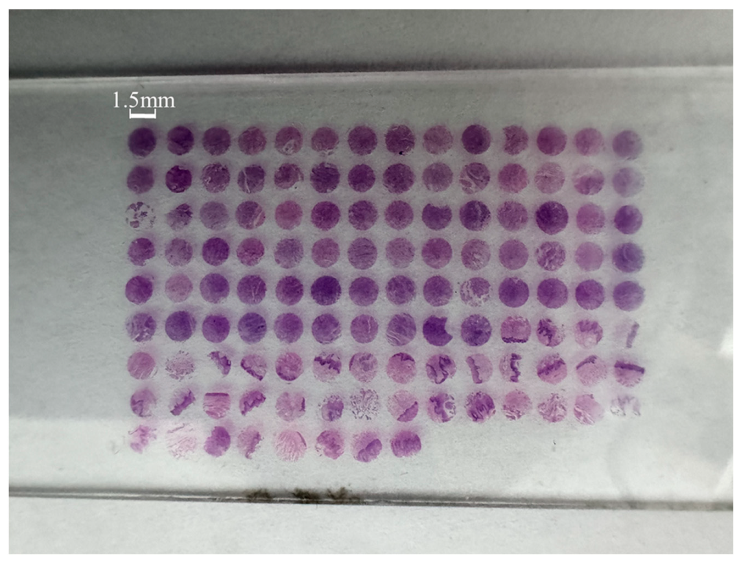
Figure 2 shows four samples in the tissue chip. Figure 2a represents normal tongue tissue, Figure 2b represents stage II tongue cancer tissue, Figure 2c represents stage III tongue cancer tissue, and Figure 2d represents stage IV tongue cancer tissue. The original microscopic images were collected by a commercial microscope (Olympus BX53M) with an objective magnification of 50×. Through the original microscopic images of the tongue tissue, it can be observed that as the tumor progresses, there are some changes in the microscopic images of each stage. However, distinguishing these changes requires pathologists to carefully observe the tissue samples to identify abnormal areas. This process is not only time-consuming but also prolongs the diagnosis time due to the limited number of pathologists.

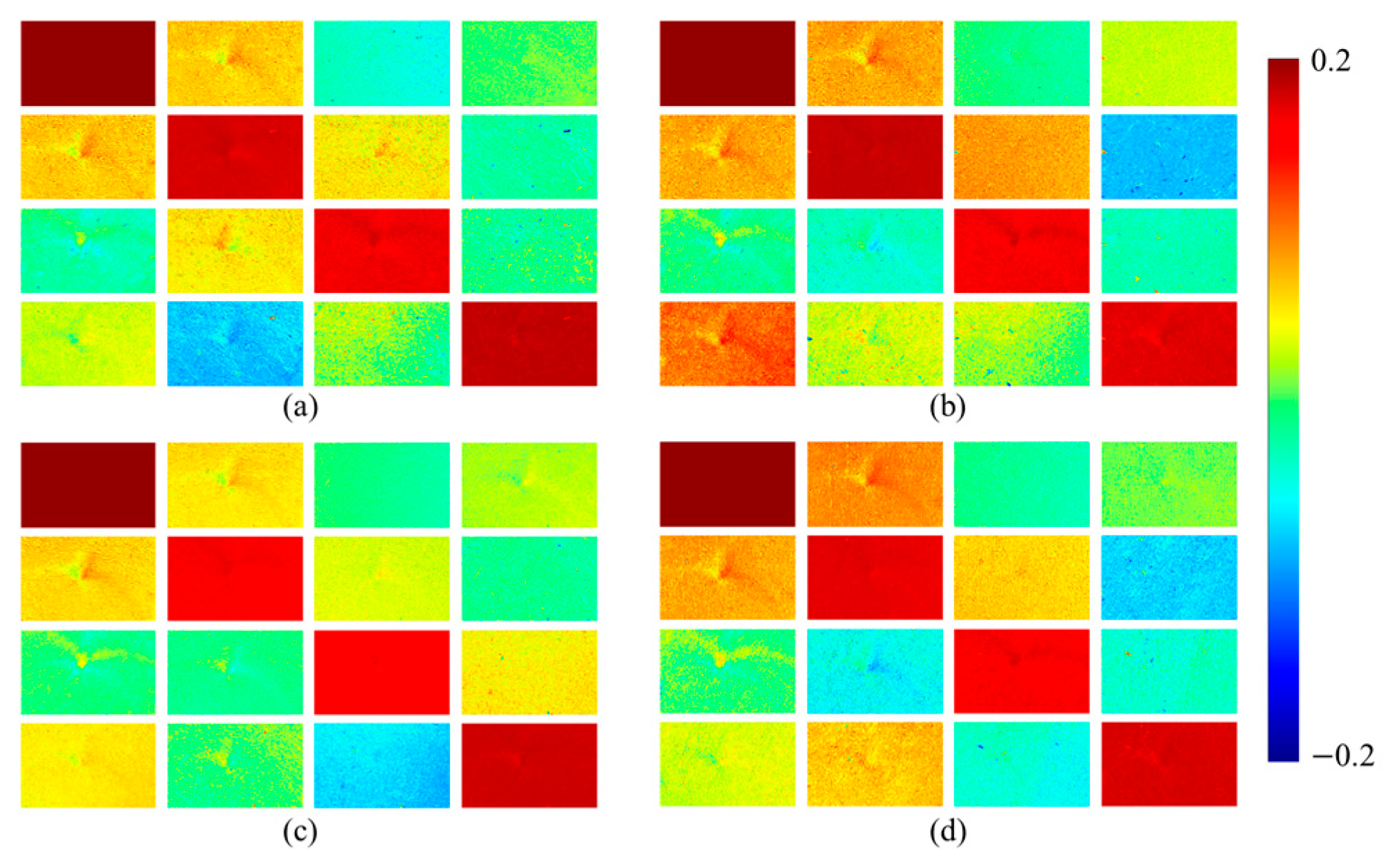
Figure 3 shows the pseudo color images of Mueller matrix elements corresponding to the four tissue samples in Figure 2. The values of the pseudo color images exhibit a clear spatial distribution between cancer tissue and normal tissue, with positive values (warm colors) representing enhanced linear birefringence and negative values (cold colors) reflecting phase delay orientation shift. The matrix elements $m_{42}$ and $m_{43}$ primarily characterize the birefringence properties of the sample. As shown in the figure, the matrix elements $m_{42}$ and $m_{43}$ exhibit noticeable differences in values between cancerous and normal tissues. The values differences between stage II and stage III tongue cancer tissues are minimal, whereas stage IV tissue shows significantly stronger values.

For $m_{43}$, there is little difference in values between normal tissue and stage II cancer tissue. However, the values become more pronounced in stage III and IV tissues. This is attributed to cancer progression, during which nuclear volume increases, collagen fibers become increasingly disordered, and the extracellular matrix exhibits greater abnormality, which can significantly affect tissue birefringence.

Although the $m_{22},m_{23}$ and $m_{44}$ images of normal and cancer tissue cannot be visually distinguished, their specific features can be obtained through deep learning. However, these parameters exhibit an inverse correlation with tissue depolarization capacity. Therefore, it is necessary to add depolarization-related parameters into the Mueller matrix parameter image dataset. $m_{12}$, $m_{13}$, $m_{21}$, and $m_{31}$ can reflect the diattenuation characteristics of the sample. Normal tongue tissue shows differences from cancer tissue at different stages, and deep learning can effectively generalize these diattenuation differences.

Although the Mueller matrix encompasses comprehensive polarization information of the sample, the physical interpretation of each individual element remains ambiguous. In order to obtain polarization parameters with interpretable physical meanings, the Mueller matrix purity introduced in Section 2.2, the Mueller matrix polar decomposition introduced in Section 2.3, and the Mueller matrix transformation introduced in Section 2.4 are further analyzed in detail. Currently, the Mueller matrix parameters that characterize the polarization characteristics of cancerous tissues mainly include the equivalent waveplate fast axis azimuth angle ($\theta$), the phase delay ($\delta$), the depolarization (Δ), the bidirectional attenuation (D), the anisotropic orientation direction ($x$), and the Mueller matrix purity ($P_{\mathrm{m}}$). After acquiring the Mueller matrix of the tongue cancer tissue chip, the Mueller matrix polar decomposition and transformation methods were used to obtain the Mueller matrix parameter images of all samples, and the $P_{\mathrm{m}}$ images of all samples were obtained using Equation (2), where the parameters derived from the Mueller matrix polar decomposition include $\theta$, $\delta$, Δ, and D and the parameter derived from the Mueller matrix transformation is $x$. Figure 4 shows the images of six Mueller matrix parameters for four types of tissue samples.

4. Establishment of Dataset

4.1. Image Cropping

Using a Mueller matrix microscope, all samples present on the chip were systematically imaged to capture detailed polarization information. In total, the dataset comprises 57 images of normal tongue tissue, 212 images of stage II tongue cancer tissue, 315 images of stage III tongue cancer tissue, and 297 images of stage IV tongue cancer tissue, as summarized in

Table 1. Sample size of raw data.

Category	Normal Tissue	Tumor Stage II	Tumor Stage III	Tumor Stage IV
Quantity	57	212	315	297

. Subsequently, for each sample, purity images, Mueller matrix polar decomposition images, and Mueller matrix transformation images were calculated separately. Each sample includes the three types of Mueller matrix parameter images mentioned above, meaning that each type of sample contains a complete Mueller matrix parameter image with a size of 3072 × 2048.

Due to the edge distortion caused by imaging principles, including optical aberrations, diffraction effects, numerical aperture limitations, and sample-related factors such as uneven sample preparation and edge effects, the original image edge quality is poor and difficult to use for subsequent analysis. Therefore, before carrying out all image processing procedures, we crop the image with a size of 3072 × 2048 to a 3000 × 2000 image to remove the edge parts.

Considering the convenience and efficiency of subsequent processing and analysis, it is necessary to further process the image that has been cropped to 3000 × 2000 and segment it into small blocks of size 200 × 200. After this cutting operation, the sample composition is as follows: 8550 normal tongue tissue samples, 31,800 stage II tongue cancer tissues, 47,250 stage III tongue cancer tissues, and 44,550 stage IV tongue cancer tissues. The final total sample size is 132150, as shown in

Table 2. Sample quantity after trimming.

Category	Normal Tissue	Tumor Stage II	Tumor Stage III	Tumor Stage IV
Quantity	8550	31,800	47,250	44,550

.

To achieve reasonable partitioning of the dataset, this study adopts a stratified sampling strategy, dividing the dataset into training set, validation set, and test set. Stratified sampling refers to sampling based on the proportion of samples from each category in the original data, ensuring that each subset maintains consistency with the original dataset in terms of category distribution, effectively avoiding data bias caused by sampling. In this study, the validation set and the test set were set to the same size, with a sample size of approximately 10% of the original data. The specific distribution is as follows: 800 normal tongue tissues, 3000 stage II tongue cancer tissues, 4000 stage III tongue cancer tissues, and 4000 stage IV tongue cancer tissues. The distribution of the training set is as follows: 6950 normal tongue tissue samples, 25,800 stage II tongue cancer tissues, 39,250 stage III tongue cancer tissues, and 36,550 stage IV tongue cancer tissues, as shown in

Table 3. Number of sample distributions after cropping.

Category	Normal Tissue	Tumor Stage II	Tumor Stage III	Tumor Stage IV
Training set	6950	25,800	39,250	36,550
Validation set	800	3000	4000	4000
Test set	800	3000	4000	4000

.

4.2. Image Resampling

In the current research dataset, there is a significant gap between the normal sample size and other categories of samples, presenting a serious problem of sample imbalance. This imbalance may lead to bias during the model training process, making the model more inclined to fit a larger number of sample category features during the learning process, resulting in insufficient feature learning for normal samples, thereby affecting the model’s recognition accuracy and overall generalization ability for normal samples.

To effectively alleviate this problem, this study uses resampling techniques to expand the number of normal samples. As a common data augmentation method, resampling adjusts the sample distribution through reasonable reuse, making it more balanced. A fourfold resampling was applied to the normal samples in the training set, increasing their count to 27,800. Similarly, stage II, III, and IV tongue cancer samples were increased to 31,800, 47,250, and 44,550, respectively, as shown in

Table 4. Distribution of resampled samples.

Category	Normal Tissue	Tumor Stage II	Tumor Stage III	Tumor Stage IV
Quantity	27,800	31,800	47,250	44,550

. At this point, the total number of samples in the training set reached 151,400. This adjustment optimizes the proportion of various types of samples in the training set, providing a more reliable data foundation for effective training of subsequent models and helping to improve the overall performance of the model in normal sample recognition and complex sample environments.

5. Results and Discussion

In the research field of medical image classification, four commonly used CNN models for medical image classification, AlexNet, ResNet50, DenseNet121 and VGGNet16, were used to test the classification accuracy of different combinations of Mueller matrix parameters for different types of tongue cancer tissues and normal tongue tissues. All four models were trained on eight NVIDIA H100 GPUs using the Aadm optimizer to minimize the cross entropy loss function. The learning rate was 0.0001, and the batch size for each GPU was 64. The number of iterations was 30. Model training uses partitioned and preprocessed training set data. To prevent overfitting, all models apply L2 regularization with a weight decay coefficient of 1 × 10⁻⁴.

The specific results of the training are presented in

Table 5. The accuracy of convolutional CNN models using different combinations of Mueller matrix parameters for classification.

Category	AlexNet	ResNet50	DenseNet121	VGGNet16
$\left\{\delta , D\right\}$	82.653%	67.144%	85.025%	86.441%
$\left\{\theta , \delta \right\}$	83.186%	77.847%	86.797%	88.669%
$\left\{\theta , \delta , D,\mathsf{\Delta }\right\}$	95.153%	96.797%	97.102%	96.127%
$\left\{\theta , \delta ,x\right\}$	93.347%	94.898%	94.517%	94.415%
$\left\{\theta , \delta , D,x\right\}$	95.068%	96.042%	96.678%	96.119%
$\left\{\theta , \delta , D,x,P_m\right\}$	95.449%	96.525%	97.373%	96.517%
$\left\{\theta , \delta , D,x,P_m,\mathsf{\Delta }\right\}$	97.737%	98.136%	98.483%	98.110%

. It is found that under these four CNN models, the parameter combination $\left\{\theta , \delta , D,x,P_m,\Delta \right\}$ corresponds to the highest level of classification accuracy, which proves that $\theta$, $\delta$, $D$, $x$, $P_{\mathrm{m}}$, and $\Delta$ can all be effective parameters for detecting tongue cancer. Among them, within the framework of the DenseNet121 model, the classification accuracy of this parameter combination is particularly outstanding, reaching 98.48%.

Figure 5 shows in detail the variation of loss values with training iterations for the four CNN models under different combinations of detection parameters. Obviously, when using the parameter combination of $\left\{\theta , \delta , D,x,P_m,\mathsf{\Delta }\right\}$, the loss value is more stable.

In other related studies on medical image classification, various methods of inputting Mueller matrix parameters have demonstrated significant outcomes. For instance, a study utilized the method of inputting a comprehensive set of multiple Mueller matrix parameters, including the 16 original matrix elements, 6 polar decomposition parameters, and 6 transformation parameters, into a convolutional neural network (CNN) for the diagnosis of osteosarcoma. This approach achieved a final accuracy of 95.79% [40]. Another study focused on classifying different types of breast cancer cells by employing 16 Mueller matrix element parameters as CNN inputs, resulting in a classification accuracy of 88.34% [41]. Furthermore, in the field of dermatological diagnostics, the application of 16 Mueller matrix element parameters as inputs to a CNN for the classification of various skin diseases yielded an accuracy as high as 98% [42]. Additionally, the use of Mueller matrix elements as CNN inputs for the detection of hepatitis B led to an accuracy rate of 90.9% [43].

However, when comparing these results with the classification performance of tongue cancer tissue using the $\left\{\theta , \delta , D,x,P_m,\mathsf{\Delta }\right\}$ parameter combinations, it becomes evident that the accuracy achieved by the latter approach is superior. This observation highlights the potential of the $\left\{\theta , \delta , D,x,P_m,\mathsf{\Delta }\right\}$ parameter combinations in achieving higher diagnostic accuracy in the specific context of tongue cancer tissue classification. Such comparative analyses underline the importance of parameter selection in enhancing the diagnostic capabilities of CNN-based medical image classification models.

Due to the fact that the parameter combination $\left\{\theta , \delta , D,x,P_m,\mathsf{\Delta }\right\}$ has the highest accuracy in tongue cancer detection among the four models, in order to further evaluate its true performance, this study combines resampling techniques and category loss weights to construct a model to explore the diagnostic efficacy of the parameter combination $\left\{\theta , \delta , D,x,P_m,\mathsf{\Delta }\right\}$. The category loss weight value is set to (normal: stage II: stage III: stage IV = 0.2820, 0.3038, 0.1997, 0.2145), and this weight is adjusted based on the number of resampled samples (the smaller the sample size, the greater the weight). Subsequently, the trained model is used to classify the images in the test dataset to evaluate the performance of the parameter combination $\left\{\theta , \delta , D,x,P_m,\mathsf{\Delta }\right\}$. Among 11,800 annotated test images, only 235 images were misclassified under the AlexNet model, 228 images were misclassified under the ResNet50 model, 130 images were misclassified under the DenseNet121 model, and 231 images were misclassified under the VGGNet16 model. The DenseNet model has the highest accuracy, about 98.90%. This once again confirms the effectiveness of deep learning polarization imaging in tongue cancer detection. To present the results more clearly, the relevant confusion matrix is shown in

Table 6. Confusion matrix of AlexNet model.

Actual Label/Predicted Label	Normal	Stage II	Stage III	Stage IV
Normal	798	0	1	1
Stage II	1	2925	53	21
Stage III	5	59	3895	41
Stage IV	2	22	29	3947

,

Table 7. Confusion matrix of ResNet50 model.

Actual Label/Predicted Label	Normal	Stage II	Stage III	Stage IV
Normal	797	1	2	0
Stage II	0	2970	21	9
Stage III	3	106	3868	23
Stage IV	4	13	46	3937

,

Table 8. Confusion matrix of DenseNet121 model.

Actual Label/Predicted Label	Normal	Stage II	Stage III	Stage IV
Normal	799	0	1	0
Stage II	1	2964	30	6
Stage III	0	47	3933	20
Stage IV	2	3	11	3974

and

Table 9. Confusion matrix of VGGNet16 model.

Actual Label/Predicted Label	Normal	Stage II	Stage III	Stage IV
Normal	796	0	3	1
Stage II	3	2950	31	16
Stage III	4	71	3892	33
Stage IV	14	24	31	39

. In addition, classification reports are included in

Table 10. Classification report including the values for precision, recall, and F1-score, evaluating AlexNet model performance.

Class	Precision	Recall	F1-Score
Normal	99.007%	99.750%	99.377%
Stage II	97.305%	97.500%	97.403%
Stage III	97.914%	97.375%	97.644%
Stage IV	98.429%	98.675%	98.552%

,

Table 11. Classification report including the values for precision, recall, and F1-score, evaluating ResNet50 model performance.

Class	Precision	Recall	F1-Score
Normal	99.129%	99.625%	99.377%
Stage II	96.117%	99.000%	97.537%
Stage III	98.247%	96.700%	97.468%
Stage IV	99.194%	98.425%	98.808%

,

Table 12. Classification report including the values for precision, recall, and F1-score, evaluating DenseNet121 model performance.

Class	Precision	Recall	F1-Score
Normal	99.750%	99.875%	99.813%
Stage II	98.016%	98.800%	98.406%
Stage III	98.943%	98.325%	98.633%
Stage IV	99.350%	99.350%	99.350%

and

Table 13. Classification report including the values for precision, recall, and F1-score, evaluating VGGNet16 model performance.

Class	Precision	Recall	F1-Score
Normal	97.430%	99.500%	98.454%
Stage II	96.880%	98.333%	97.601%
Stage III	98.357%	97.300%	97.826%
Stage IV	98.744%	98.275%	98.509%

, which evaluate the accuracy, recall, and F1-score of each category as classification metrics. From the tables, it can be seen that these indicators maintain similar and large values among various categories, indicating that parameter combination $\left\{\theta , \delta , D,x,P_m,\mathsf{\Delta }\right\}$ has good classification performance.

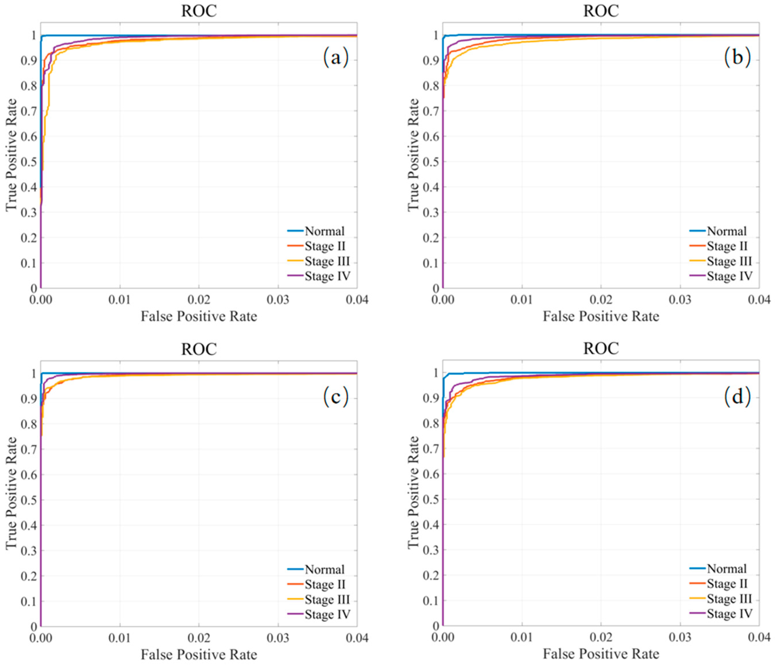
Finally, the receiver operating characteristic (ROC) curves for all tongue cancer tissue classes are shown in Figure 6, again confirming the good classification capabilities of the model for all classes.

In addition, we also used Grad-CAM to display which regions of normal tongue tissue and stage II, III, and IV tongue cancer tissue images are most relevant to the model. Figure 7a–d show images of normal tongue tissue and stage II, III, and IV tongue cancer tissue, respectively. Note that the left subimage of each figure is a microscopic image, while the right subimage corresponds to a Grad-CAM image. Normal tongue tissue is a highly ordered structure; therefore, in Grad-CAM images, differentiated mature, morphological regularity, orderly arranged cells, and clear stratification (epithelium, lamina propria, muscle) are the main features. The main features of Grad-CAM images in tongue cancer tissues are highly heterogeneous and malignant characteristics of cells (varying sizes and shapes, abnormal nuclei, active division), complete disorder and destruction of tissue structure, and loss of normal stratification and polarity. The most crucial thing is that cancer cells break through the limitations of the basement membrane and have the ability to infiltrate and grow, invading and destroying deep tissues (lamina propria, muscles). This uncontrolled invasive growth and destructive nature are essential features of cancer.

In summary, through the comparative analysis of multiple experimental results, the significant superiority of this diagnostic parameter combination in the field of medical image classification has been fully verified. In view of this, the combination of diagnostic parameters not only has extremely high application value in the diagnosis of tongue cancer tissue but also has great potential to expand to other meaningful pathological tissue classification work and is expected to provide more accurate and effective technical support for the field of medical diagnosis.

6. Conclusions

This study successfully integrated MMM imaging with deep learning to achieve efficient classification of tongue cancer tissue chips. By selecting key combinations of polarization parameter $\left\{\theta , \delta , D,x,P_m,\mathsf{\Delta }\right\}$, a classification accuracy of 98.48% was achieved in the DenseNet121 model, which is significantly improved compared to traditional methods. Experimental results demonstrate that Mueller matrix parameters can characterize the microstructural changes in the evolution of tongue cancer, with optical properties closely aligned with polarization imaging. Compared to existing research, this method demonstrates significant advantages in parameter selection and network adaptability.

References

1. Moore, S.R.; Johnson, N.W.; Pierce, A.M.; Wilson, D.F. The epidemiology of tongue cancer: A review of global incidence. Oral Dis. 2000, 6, 75–84. [Google Scholar] [CrossRef]
2. Sessions, D.G.; Spector, G.J.; Lenox, J.; Haughey, B.; Chao, C.; Marks, J. Analysis of treatment results for oral tongue cancer. Laryngoscope 2002, 112, 616–625. [Google Scholar] [CrossRef] [PubMed]
3. Rana, A.; Lowe, A.; Lithgow, M.; Horback, K.; Janovitz, T.; Da Silva, A.; Tsai, H.; Shanmugam, V.; Bayat, A.; Shah, P. Use of deep learning to develop and analyze computational hematoxylin and eosin staining of prostate core biopsy images for tumor diagnosis. JAMA Netw. Open 2020, 3, e205111. [Google Scholar] [CrossRef]
4. Wu, H.H.; Jovonovich, S.M.; Randolph, M.; Post, K.M.; Sen, J.D.; Curless, K.; Cheng, L. Utilization of cell-transfer technique for molecular testing on hematoxylin-eosin–stained sections: A viable option for small biopsies that lack tumor tissues in paraffin block. Arch. Pathol. Lab. Med. 2016, 140, 1383–1389. [Google Scholar] [CrossRef]
5. Tashiro, A.; Sano, M.; Kinameri, K.; Fujita, K.; Takeuchi, Y. Comparing mass screening techniques for gastric cancer in Japan. World J. Gastroenterol. 2006, 12, 4873–4874. Available online: https://pmc.ncbi.nlm.nih.gov/articles/PMC4087623/ (accessed on 15 June 2025).
6. Ganly, I.; Patel, S.; Shah, J. Early stage squamous cell cancer of the oral tongue—Clinicopathologic features affecting outcome. Cancer 2012, 118, 101–111. [Google Scholar] [CrossRef]
7. Hsiao, T.Y.; Lee, S.Y.; Sun, C.W. Optical polarimetric detection for dental hard tissue diseases characterization. Sensors 2019, 19, 4971. [Google Scholar] [CrossRef] [PubMed]
8. Cacace, T.; Bianco, V.; Ferraro, P. Quantitative phase imaging trends in biomedical applications. Opt. Lasers Eng. 2020, 135, 106188. [Google Scholar] [CrossRef]
9. Park, Y.K.; Depeursinge, C.; Popescu, G. Quantitative phase imaging in biomedicine. Nat. Photonics 2018, 12, 578–589. [Google Scholar] [CrossRef]
10. Tsai, C.L.; Mukundan, A.; Chung, C.S.; Chen, Y.H.; Wang, Y.K.; Chen, T.H.; Tseng, Y.S.; Huang, C.W.; Wu, I.C.; Wang, H.C. Hyperspectral imaging combined with artificial intelligence in the early detection of esophageal cancer. Cancers 2021, 13, 4593. [Google Scholar] [CrossRef]
11. Karim, S.; Qadir, A.; Farooq, U.; Shakir, M.; Laghari, A.A. Hyperspectral imaging: A review and trends towards medical imaging. Curr. Med. Imaging Rev. 2023, 19, 417–427. [Google Scholar] [CrossRef]
12. Yang, L.; Chen, Y.; Ling, S.; Wang, J.; Wang, G.; Zhang, B.; Zhao, H.; Zhao, Q.; Mao, J. Research progress on the application of optical coherence tomography in the field of oncology. Front. Oncol. 2022, 12, 953934. [Google Scholar] [CrossRef]
13. Schwartz, D.; Sawyer, T.W.; Thurston, N.; Barton, J.; Ditzler, G. Ovarian cancer detection using optical coherence tomography and convolutional neural networks. Neural Comput. Appl. 2022, 34, 8977–8987. [Google Scholar] [CrossRef]
14. Wang, Y.; He, H.; Chang, J.; He, C.; Liu, S.; Li, M.; Zeng, N.; Wu, J.; Ma, H. Mueller matrix microscope: A quantitative tool to facilitate detections and fibrosis scorings of liver cirrhosis and cancer tissues. J. Biomed. Opt. 2016, 21, 071112. [Google Scholar] [CrossRef] [PubMed]
15. Dong, Y.; Qi, J.; He, H.; He, C.; Liu, S.; Wu, J.; Elson, D.S.; Ma, H. Quantitatively characterizing the microstructural features of breast ductal carcinoma tissues in different progression stages by Mueller matrix microscope. Biomed. Opt. Express 2017, 8, 3643–3655. [Google Scholar] [CrossRef] [PubMed]
16. Bray, F.; Ferlay, J.; Soerjomataram, I.; Siegel, R.L.; Torre, L.A.; Jemal, A. Global cancer statistics 2018: GLOBOCAN estimates of incidence and mortality worldwide for 36 cancers in 185 countries. CA Cancer J. Clin. 2018, 68, 394–424. [Google Scholar] [CrossRef] [PubMed]
17. Sung, H.; Ferlay, J.; Siegel, R.L.; Laversanne, M.; Soerjomataram, I.; Jemal, A.; Bray, F. Global cancer statistics 2020: GLOBOCAN estimates of incidence and mortality worldwide for 36 cancers in 185 countries. CA Cancer J. Clin. 2021, 71, 209–249. [Google Scholar] [CrossRef] [PubMed]
18. Siegel, R.L.; Miller, K.D.; Jemal, A. Cancer statistics, 2019. CA Cancer J. Clin. 2019, 69, 7–34. [Google Scholar] [CrossRef]
19. Meng, Q.; Shi, S.; Liang, C.; Liang, D.; Xu, W.; Ji, S.; Zhang, B.; Ni, Q.; Xu, J.; Yu, X. Diagnostic and prognostic value of carcinoembryonic antigen in pancreatic cancer: A systematic review and meta-analysis. OncoTargets Ther. 2017, 10, 4591–4598. [Google Scholar] [CrossRef]
20. Zhou, J.M.; Wang, T.; Zang, K.H. AFP-L3 for the diagnosis of early hepatocellular carcinoma: A meta-analysis. Medicine 2021, 100, e27673. [Google Scholar] [CrossRef]
21. Hanke, R.; Fuchs, T.; Uhlmann, N. X-ray based methods for non-destructive testing and material characterization. Nucl. Instrum. Methods. Phys. Res. A 2008, 591, 14–18. [Google Scholar] [CrossRef]
22. Tashman, S.; Anderst, W. In vivo measurement of dynamic joint motion using high speed biplane radiography and CT: Application to canine ACL deficiency. J. Biomech. Eng. 2003, 125, 238–245. [Google Scholar] [CrossRef]
23. Kidwell, C.S.; Saver, J.L.; Villablanca, J.P.; Duckwiler, G.; Fredieu, A.; Gough, K.; Leary, M.C.; Starkman, S.; Gobin, Y.P.; Jahan, R.; et al. Magnetic resonance imaging detection of microbleeds before thrombolysis: An emerging application. Stroke 2002, 33, 95–98. [Google Scholar] [CrossRef]
24. Wortsman, X.; Alfageme, F.; Roustan, G.; Arias-Santiago, S.; Martorell, A.; Catalano, O.; Scotto di Santolo, M.; Zarchi, K.; Bouer, M.; Gonzalez, C.; et al. Guidelines for performing dermatologic ultrasound examinations by the DERMUS group. J. Ultrasound Med. 2016, 35, 577–580. [Google Scholar] [CrossRef]
25. Zhu, L.; Zhang, H.; Gu, H.; Zhou, J. The pathology biopsy represents the “gold standard” for diagnosis: A case report. Diagn. Microbiol. Infect. Dis. 2024, 108, 116138. [Google Scholar] [CrossRef] [PubMed]
26. Liu, T.; Lu, M.; Chen, B.; Zhong, Q.; Li, J.; He, H.; Mao, H.; Ma, H. Distinguishing structural features between Crohn’s disease and gastrointestinal luminal tuberculosis using Mueller matrix derived parameters. J. Biophotonics 2019, 12, e201900151. [Google Scholar] [CrossRef] [PubMed]
27. Huang, T.; Yao, Y.; Pei, H.; Hu, Z.; Zhang, F.; Wang, J.; Yu, G.; Huang, C.; Liu, H.; Tao, L.; et al. Mueller matrix imaging of pathological slides with plastic coverslips. Opt. Express 2023, 31, 15682–15696. [Google Scholar] [CrossRef]
28. Singh, A.; Sau, A.K. Tissue microarray: A powerful and rapidly evolving tool for high-throughput analysis of clinical specimens. Int. J. Case Rep. Images 2010, 1, 1–6. [Google Scholar] [CrossRef]
29. Vassella, E.; Galván, J.A.; Zlobec, I. Tissue microarray technology for molecular applications: Investigation of cross-contamination between tissue samples obtained from the same punching device. Microarrays 2015, 4, 188–195. [Google Scholar] [CrossRef]
30. Deng, L.; Chen, C.; Yu, W.; Shao, C.; Shen, Z.; Wang, Y.; He, C.; Li, H.; Liu, Z.; He, H.; et al. Influence of hematoxylin and eosin staining on linear birefringence measurement of fibrous tissue structures in polarization microscopy. J. Biomed. Opt. 2023, 28, 102909. [Google Scholar] [CrossRef]
31. Wood, M.F.G.; Vurgun, N.; Wallenburg, M.A.; Vitkin, I.A. Effects of formalin fixation on tissue optical polarization properties. Phys. Med. Biol. 2011, 56, N115. [Google Scholar] [CrossRef]
32. Wei, H.; Zhou, Y.; Ma, F.; Yang, R.; Liang, J.; Ren, L. Full-automatic high-efficiency Mueller Matrix microscopy imaging for tissue microarray inspection. Sensors 2024, 24, 4703. [Google Scholar] [CrossRef]
33. Gil, J.J.; Eusebio, B. A depolarization criterion in Mueller matrices. Opt. Acta 1985, 32, 259–261. [Google Scholar] [CrossRef]
34. Lu, S.Y.; Chipman, R.A. Interpretation of Mueller matrices based on polar decomposition. J. Opt. Soc. Am. A 1996, 13, 1106–1113. [Google Scholar] [CrossRef]
35. He, H.; Zeng, N.; Du, E.; Guo, Y.; Li, D.; Liao, R.; Ma, H. A possible quantitative Mueller Matrix transformation technique for anisotropic scattering media. Photonics Lasers Med. 2013, 2, 129–137. [Google Scholar] [CrossRef]
36. Krizhevsky, A.; Sutskever, I.; Hinton, G.E. ImageNet classification with deep convolutional neural networks. Commun. ACM 2017, 60, 84–90. [Google Scholar] [CrossRef]
37. He, K.; Zhang, X.; Ren, S.; Sun, J. Deep residual learning for image recognition. In Proceedings of the IEEE Conference on Computer Vision and Pattern Recognition. In Proceedings of the IEEE Conference on Computer Vision and Pattern Recognition (CVPR), Las Vegas, NV, USA, 27–30 June 2016. [Google Scholar] [CrossRef]
38. Simonyan, K.; Zisserman, A. Very deep convolutional networks for large-scale image recognition. Comput. Sci. 2014, 1409, 1556. [Google Scholar] [CrossRef]
39. Huang, G.; Liu, Z.; Van Der Maaten, L.; Weinberger, K.Q. Densely connected convolutional networks. In Proceedings of the IEEE Conference on Computer Vision and Pattern Recognition, Honolulu, HI, USA, 21–26 July 2017. [Google Scholar] [CrossRef]
40. Zhao, Y.; Reda, M.; Feng, K.; Zhang, P.; Cheng, G.; Ren, Z.; Kong, S.G.; Su, S.; Huang, H.; Zang, J. Detecting giant cell tumor of bone lesions using Mueller matrix polarization microscopic imaging and multi-parameters fusion network. IEEE Sens. J. 2020, 20, 7208–7215. [Google Scholar] [CrossRef]
41. Xia, L.; Yao, Y.; Dong, Y.; Wang, M.; Ma, H.; Ma, L. Mueller polarimetric microscopic images analysis based classification of breast cancer cells. Opt. Commun. 2020, 475, 126194. [Google Scholar] [CrossRef]
42. Ivanov, D.; Zaharieva, L.; Mircheva, V.; Troyanova, P.; Terziev, I.; Ossikovski, R.; Novikova, T.; Genova, T. Polarization-based digital histology of human skin biopsies assisted by deep learning. Photonics 2024, 11, 185. [Google Scholar] [CrossRef]
43. Pham, T.T.H.; Nguyen, H.P.; Luu, T.N.; Le, N.B.; Vo, V.T.; Huynh, N.T.; Phan, Q.H.; Le, T.H. Combined Mueller matrix imaging and artificial intelligence classification framework for Hepatitis B detection. J. Biomed. Opt. 2022, 27, 075002. [Google Scholar] [CrossRef] [PubMed]
Figure 1. Images of mixed tissue chips of normal tongue tissue and stage II, stage III, and stage IV tongue cancer tissues.
Optics 06 00035 g001
Figure 2. Original microscopic image of tongue tissue. (a) Normal tongue tissue; (b) stage II tongue cancer tissue; (c) stage III tongue cancer tissue; (d) stage IV tongue cancer tissue.
Optics 06 00035 g002
Figure 3. Tongue tissue Mueller matrix element images. (a) Normal tongue tissue; (b) stage II tongue cancer tissue; (c) stage III tongue cancer tissue; (d) stage IV tongue cancer tissue. Between different organizations, subtle differences in intensity can be observed for m 22 ,   m 23 , and m 44 , while significant differences in intensity can be observed for m 42 and m 43 .
Optics 06 00035 g003
Figure 4. Tongue tissue Mueller matrix parameters images. (a) Normal tongue tissue; (b) stage II tongue cancer tissue; (c) stage III tongue cancer tissue; (d) stage IV tongue cancer tissue.
Optics 06 00035 g004
Figure 5. Loss value variations of training sets with different Mueller matrix parameter combinations under four CNN models. (a) AlexNet model; (b) ResNet50 model; (c) DenseNet121 model; (d) VGGNet16 model.
Optics 06 00035 g005
Figure 6. ROC curves for tongue tissue classification using four CNN models. (a) AlexNet model; (b) ResNet50 model; (c) DenseNet121 model; (d) VGGNet16 model.
Optics 06 00035 g006
Figure 7. Grad-CAM images of tongue tissue. (a) Normal tongue tissue; (b) stage II tongue cancer tissue; (c) stage III tongue cancer tissue; (d) stage IV tongue cancer tissue.
Optics 06 00035 g007