Lidar-Based Spatial Large Deflection Measurement System for Wind Turbine Blades

Abstract

With the advancement of China’s wind power industry, research into full-scale structural testing of wind turbine blades, including static testing and fatigue testing, has shown increasing significance. Static testing measures the deflection at fixed points, using pull-wire sensors in industrial practice. However, the demerits of this method involve single dimension, excessive deviation, costly experiment, and complex installment. Given the advantages that lidar provides, correspondingly, high data density, precision, and convenience, we proposed a simple and efficient spatial large deflection measurement system for wind turbine blades with multi lidars. For point clouds collected from lidar scanners, registration based on point primitives and geometric primitives, dynamic radius DBSCAN clustering, spatial line clustering, and line integrals are applied to calculate the 3D coordinates of measured points on the blade. Experimentally validated, the proposed method demonstrates its effectiveness in serving as a viable alternative to the traditional pull-wire sensor measurement approach. In the minimum oscillation direction test, the measurement error is controlled within 3% compared to the theoretical value. Simultaneously, in the maximum swing direction test, the 3D coordinates of the measured point remain consistent with the changing trend observed under small deformation. These results confirm the feasibility of the system and its potentials to be generalized.

1. Introduction

In the context of rapid growth in global energy demand, an increasing priority is given to issues such as environmental pollution, energy supply and demand, and energy structure [1], which affect not only the efficient use of energy but also its sustainable development. With the international community’s net zero emissions protocol, China has proposed the Double Carbon goal to peak carbon emissions and reach carbon neutrality [2]. Wind energy, as a natural resource, is currently one of the most promising and non-polluting renewable energy sources [3]. The core of wind power generation is the wind turbine, consisting of blades, towers, transmission structures, and power generation systems [4]. The blades play a crucial role, in that the power generated by wind energy is directly proportional to the contact area of the blades; in other words, longer blades result in greater capture of input power. To better adapt to modern energy demands, blades are required to develop towards larger and lighter structures, having progressed from 30 m in the mid-1990s to over 100 m at present [5]. However, as the blades lengthen, their structural properties change, leading to a decrease in bending stiffness [6] and a heightened susceptibility to deformations [7]. Furthermore, wind farms are primarily located in regions abundant with wind resources, the downside of which could be extremely harsh environmental conditions. This means that these turbines must afford powerful wind loads, ultraviolet erosion, and corrosion from rain and snow throughout the year, prone to abrasion, iced-over surface, cracks, and fractures [8]. They thus contribute to diminished power efficiency, elevated maintenance costs, and, in severe cases, pose potential safety risks [9]. Hence, to ensure that the design and production of blades meet the expected strength and lifespan [10], it is crucial to conduct full-scale structural testing on large wind turbine blades, including static and fatigue testing. Static testing, namely, a method that validates blade design and safety under static loads [11], employs deflection as a main source of assessment.

Present day research divides methods for the full-scale static testing of wind turbine blades into two types. The first one is contact-based, such as measuring tapes [12], pull-wire sensors, and strain sensors [13]. In 2014, Wang Chao et al. [12] determined the deflection of the blade with tapes fixed to the measurement points. However, both the tape and pull-wire sensor measure a single dimension of deflection, resulting in significant errors during severe blade deformations. In 2017, Kyunghyun Lee [13] introduced a strain-based displacement estimation method and an objective function for optimal sensor placement. Across diverse testing scenarios, the outcomes of estimation matched the measured values. Moreover, the strain method is able to estimate loading conditions and identify abnormalities like cracks through signal processing, though it is typically suited for microscopic deformations at critical points of the blade; in other words, it has a restricted range of measurement. As the number of measurement points increases, the layout of the sensors becomes highly complex, not to mention that all contact sensor measurements are prone to failure under cyclic loading. The second type is non-contact, such as multi-group vision [14], Ultra-Wideband wireless ranging (UWB) [15], total stations [6], etc. In 2012, Jinshui Yang [14] introduced visual measurement, which involves attaching grid points to the blade, using multiple cameras to capture images of these points from various angles, and triangulating their three-dimensional coordinates. However, this method relies heavily on the quality of the original image and its processing, meaning that lighting and texture greatly influence the results. In 2021, Xiao Liang [15] constructed the UWB measurement system that communicates with three base stations by transmitting tag signals, then applied the spherical intersection method to compute the three-dimensional coordinates of the tag points on the blade. Total station measurement ensures high accuracy, yet it is labor-intensive, inefficient, and cannot measure at high frequencies. Defects in the above-mentioned methods have blocked their ways towards practical applications.

In the present day, lidar is probably the synonym for high data density, precision, and measurement frequency. Being both flexible and lightweight, it is not constrained by steep angles or shadows. Its outstanding performance stretches to the fields of unmanned driving [16] and forest monitoring [17], and it has applications in modeling and mapping, such as bridge deformation monitoring [18,19,20], tunnel safety monitoring [21], and wind turbine monitoring [22,23,24]. High-resolution lidar is often chosen for monitoring bridge deformation [18,19,20], that is, the three-dimensional laser scanner is capable of acquiring point cloud data of high-density objects, though the cost of it is high. In 2017, Ivan Nikolov et al. [22] employed RPLIDAR and a 9-DOF Inertial Measurement Unit (IMU) for positioning and mapping. They geometrically simplified the two-dimensional cross-section of the wind turbine blade into an elliptical model for distance and shape correction. Limitations of this research include focusing solely on static blades, lacking analysis of dynamic scenes. Also, the research collected position information via lidar but had yet to take into consideration the overall shape information of the blade. In 2020, Luo Wei et al. [23] designed a cost-effective version of lidar to test on a blade 75 cm long. They acquired depth images of the blade model under various bending deformations and calculated the deflection deformation. However, they only built a small test bench and lacked research on modifications according to the actual test scene.

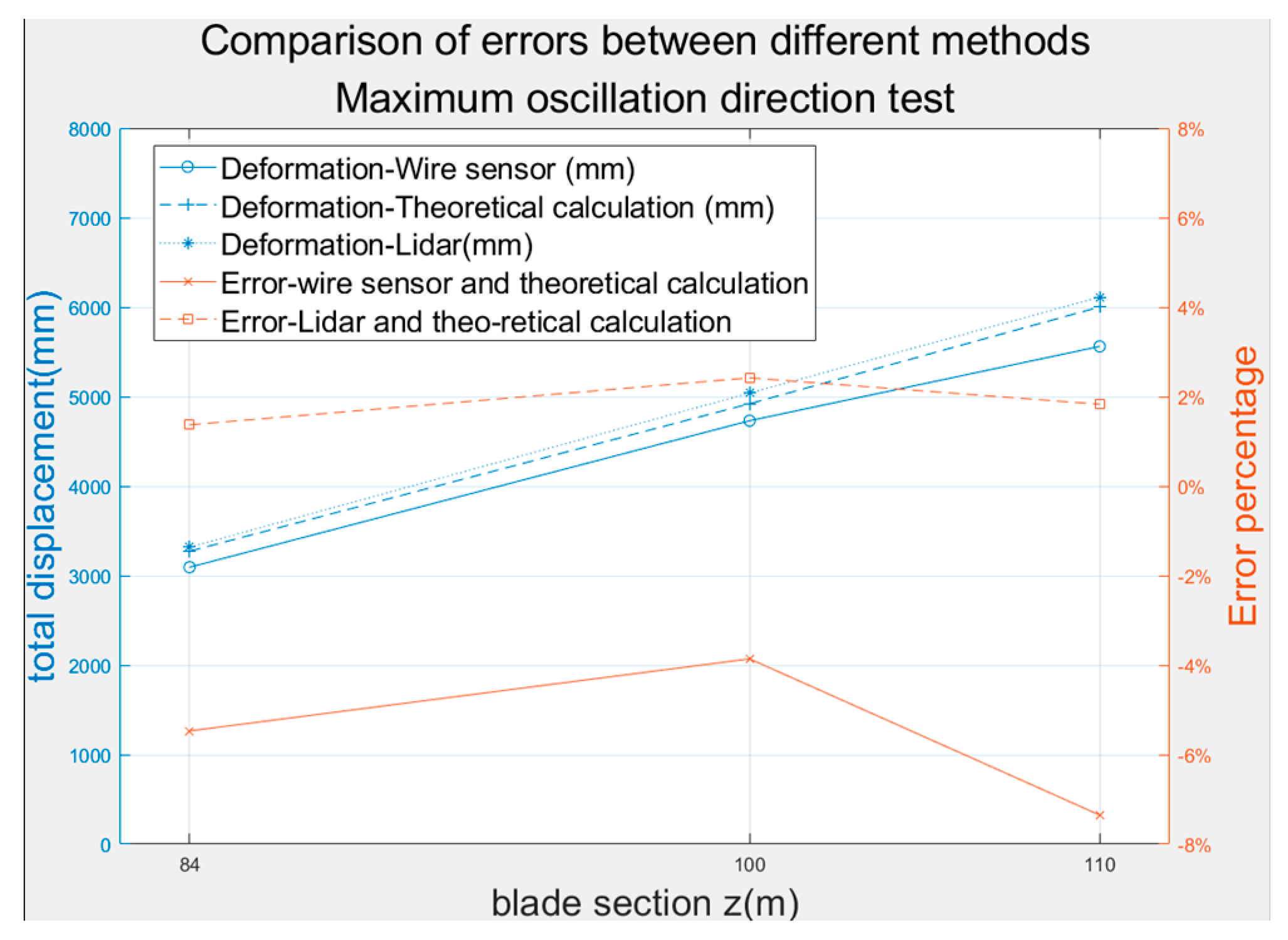
We proposed an effective and simple cost-effective multi-lidar deflection measurement method based on the actual blade in full-scale measurement scenarios. It involves using lidar [25,26] as the main equipment, incorporating novel point cloud data processing techniques such as point cloud registration on a point and geometric primitive basis, spatial clustering with dynamic radius, and spatial line clustering. Experimentally validated, the proposed method is easy to use without physical contact and demonstrates its effectiveness in serving as a viable alternative to the traditional pull-wire sensor measurement approach. In the minimum oscillation direction test, the measurement error is controlled within 3% compared to the theoretical value. Simultaneously, in the maximum swing direction test, the 3D coordinates of the measured point remain consistent with the variation trend observed under small deformation. These results confirm the feasibility of the system and its potential to be generalized.

2. Point Cloud Data Processing

The entire process is divided into four steps: experimental setup, process of experimentation, data post-processing, and analysis and summary, respectively, as shown in Figure 1.

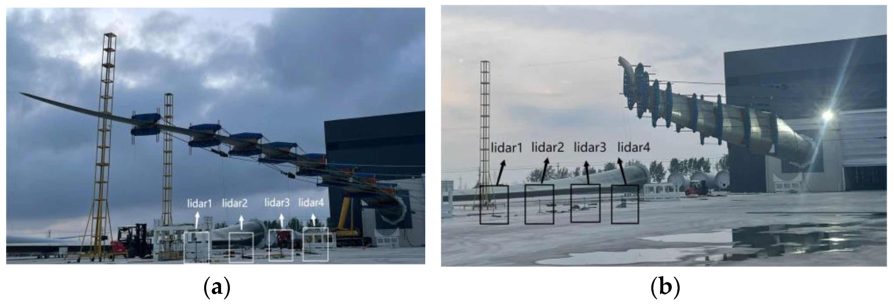
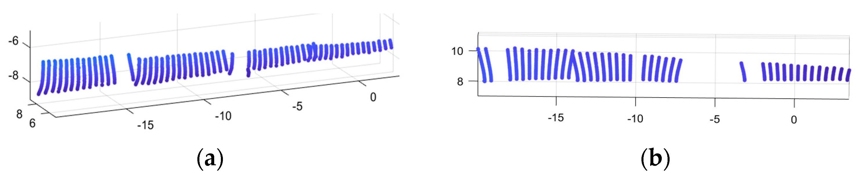
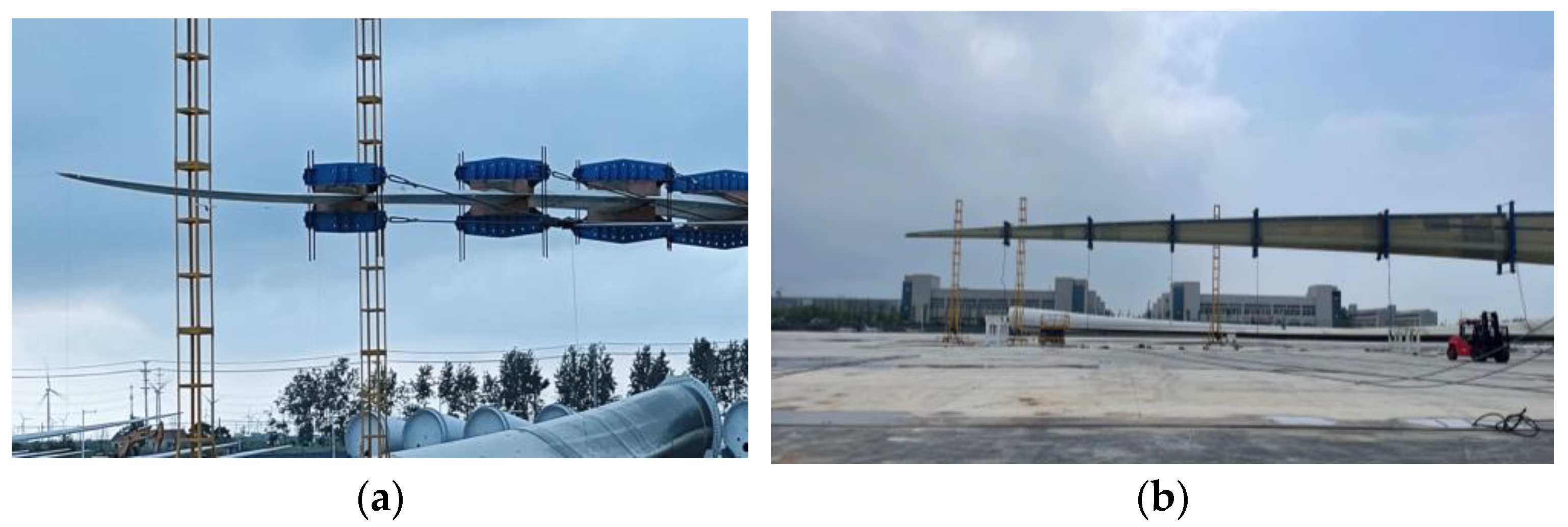
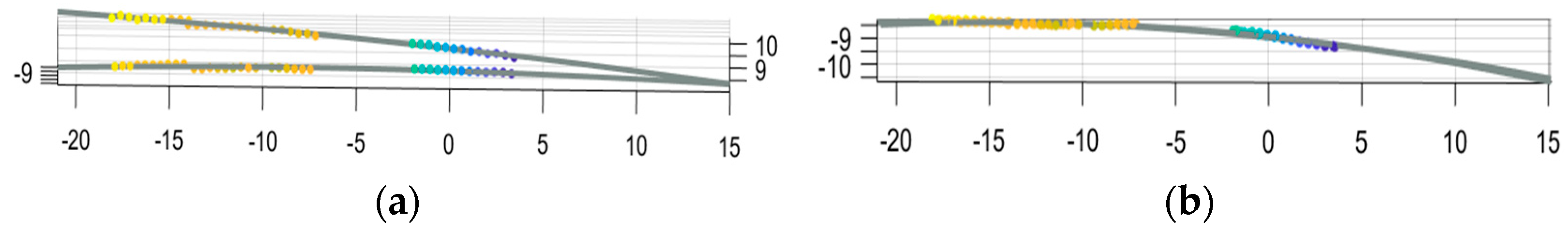
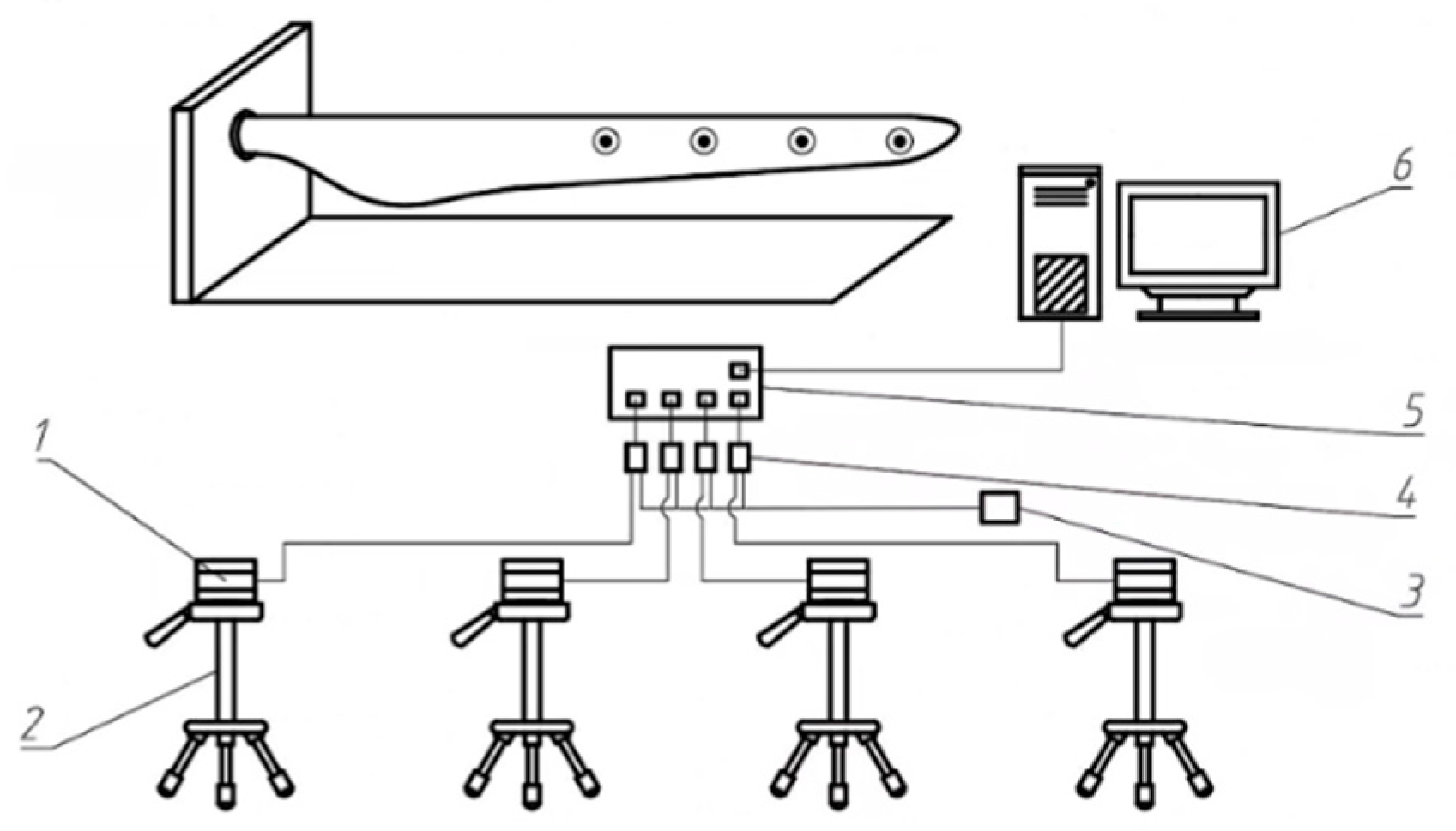
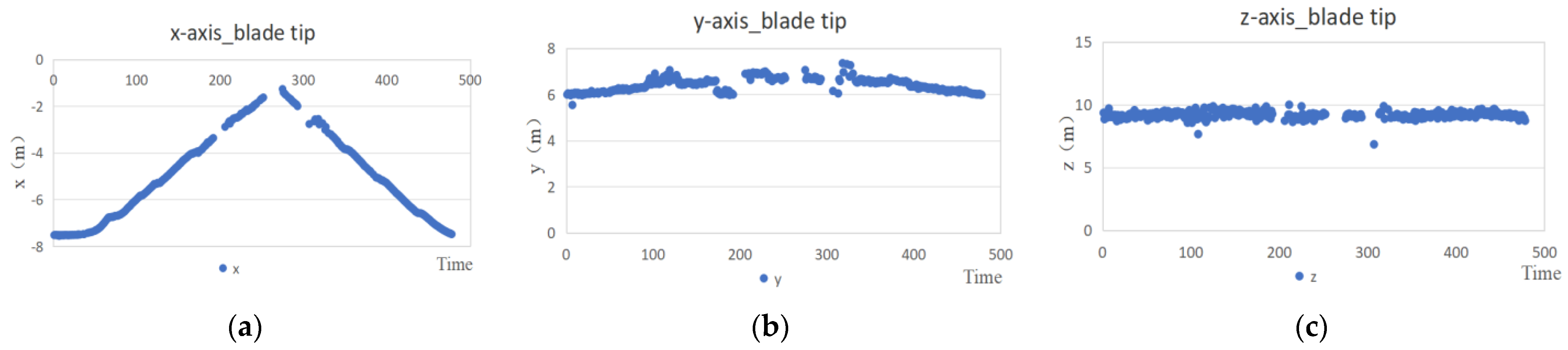
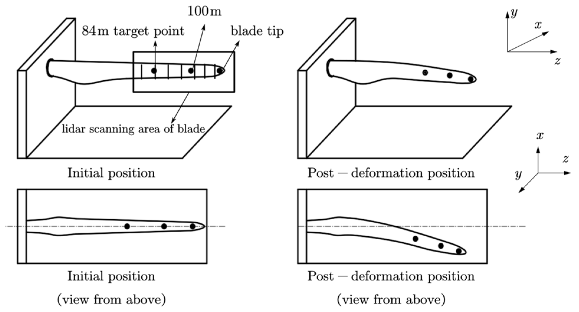
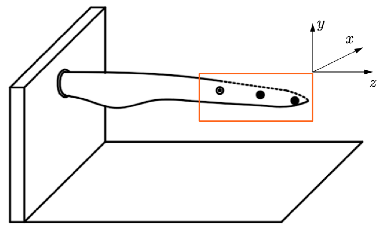
The test scene is an open outdoor area and the total length of the blade is 110 m. Two sets of tests are included: the minimum oscillation direction test and the maximum swing direction test, as shown in Figure 2a,b and Figure 3a,b. The world coordinate system identifies the test bench as its original point and conforms to the right-hand rule: the x-axis represents the horizontal direction, the y-axis represents the direction perpendicular to the ground, and the z-axis represents the direction of the blade axis, as shown in Figure 4.

Theoretically, the pull-wire sensor could be installed at any position on the blade, but in static tests, we paid more attention to the areas where variations in blade deflections are relatively larger. Therefore, we chose three target points: 84 m, 100 m, and 110 m away from the blade root. Similarly, four lidars are arranged at a certain distance on the ground, starting from the blade tip. We placed the lidars vertically at 90$°$ to obtain denser point cloud data from the blade. The scanning line on the blade is shown in the framed area in Figure 4. Upon completion of data acquisition, the point clouds undergo various techniques of post-processing; thus, the 3D coordinates of the three target measured points are calculated. In the end, the measurement data from the lidar and pull-wire sensor are respectively compared with theoretical simulation values.

2.1. Multi-Lidar Point Cloud Registration

The lidar-based deflection measurement system contains multiple lidar devices. Each lidar’s point cloud data is built on its own internal coordinate system. Point cloud registration, necessary for establishing correlations among data from multiple lidars, is about discovering the rigid transformation matrix across multiple lidar coordinate systems. The input is two frames of point cloud data from different spatial locations at the same time, marked as source point cloud ${X^s=\{x}_i^s\}$ and target point cloud ${X^t=\{x}_i^t\},\mathrm{r}\mathrm{e}\mathrm{s}\mathrm{p}\mathrm{e}\mathrm{c}\mathrm{t}\mathrm{i}\mathrm{v}\mathrm{e}\mathrm{l}\mathrm{y}$. A rotation matrix R and a translation vector T are obtained from point cloud registration; thus, coordinates of the source point cloud and the target point cloud are combined and corresponded, as shown in Formula (1):

$$\begin{array}{c}{x}_i^{s^{\prime }}=R\times x_i^s+T\end{array}$$

(1)

Point cloud registration can be divided into three major categories: point primitive, geometric primitive, and voxel primitive. Due to the specificity of blade deflection measurement scenarios and the relatively small number of lidar hardware channels, we proposed a registration method of hybrid primitives, which combines geometric primitives and point primitives to achieve the purpose of registration.

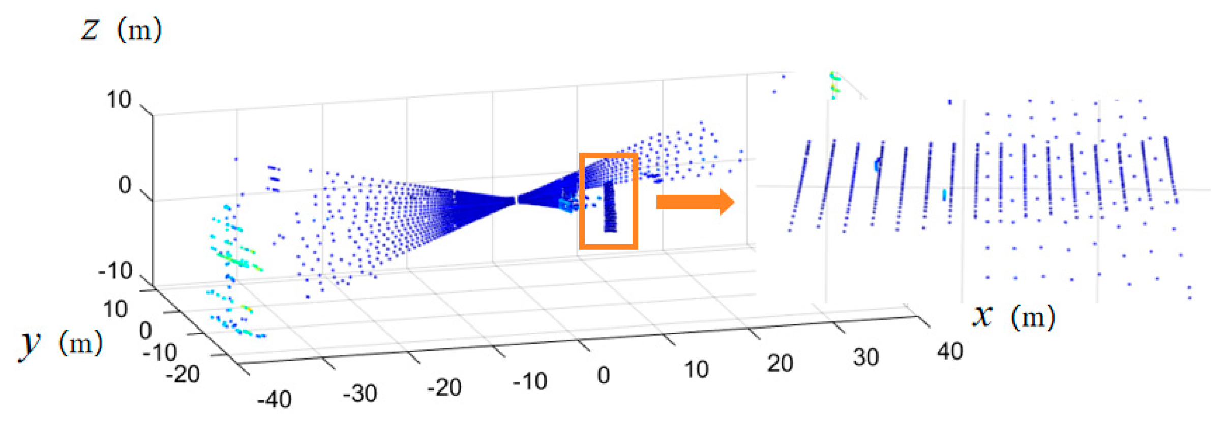
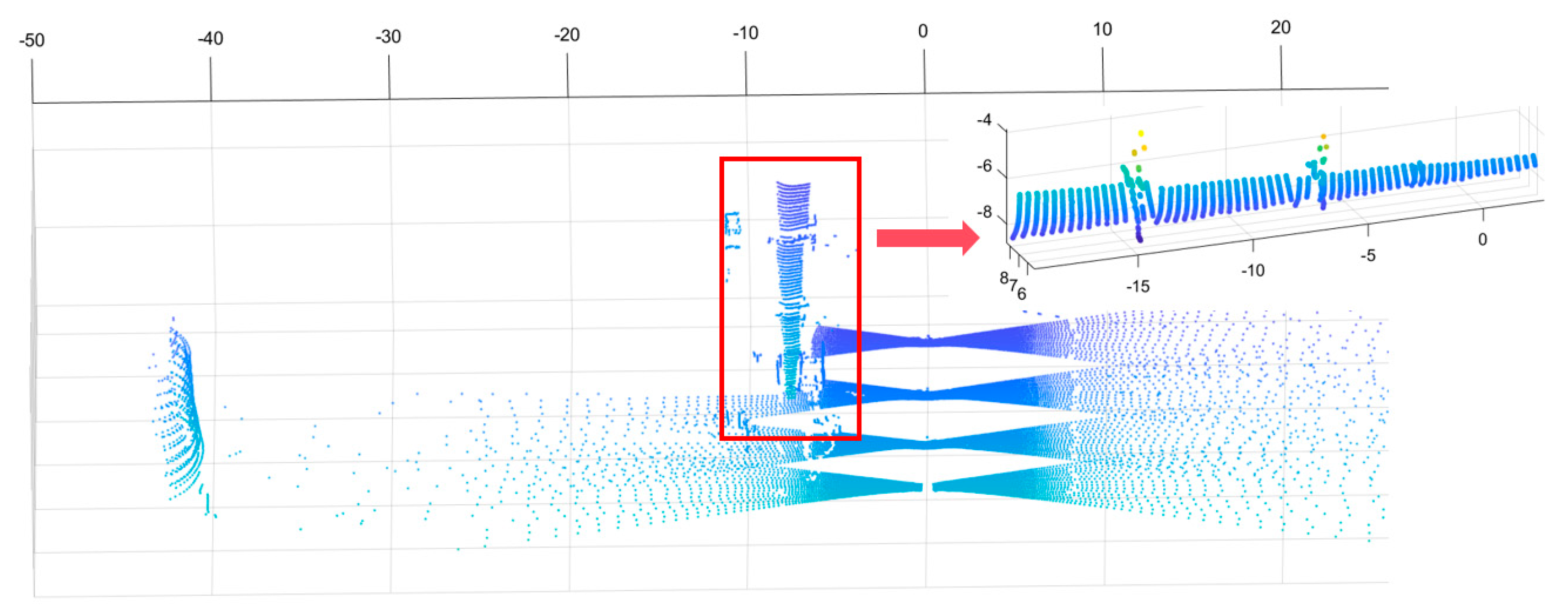
The host computer collects data, and the point cloud image of the test scene in Figure 2a is shown in Figure 5.

We used point primitives to calculate the translation vector and geometric primitives to calculate the rotation matrix. Point primitives set up pairs of points between the source point clouds and target point clouds to complete the transformation. As for achieving translational registration, we referred to the average distance between the vertices of each support frame, measured multiple times under experiment scene settings.

Straight lines or planes with stronger semantics serve as the basis for the registration method based on geometric primitives, such as the ground and walls in the blade test scene. Geometric primitives exhibit better robustness under special test scenarios of blades.

As shown in Figure 5, the ground point cloud is not parallel to any coordinate plane and has a significant slope. Applying the x-, y-, and z-axes for direct segmentation may easily mix in point cloud data from other objects. Therefore, the distance between the point cloud and the center point of the lidar was determined as a yardstick for segmentation. The effect is shown in Figure 6 below:

After the segmentation, it is necessary to detect the point cloud in the feature plane and then complete extraction. The collection of ground point cloud data is $\{p_1\left(x_1,y_1,z_1\right),p_2\left(x_2,y_2,z_2\right),\dots ,p_n(x_n,y_n,z_n\left)\right\}$. The fitted Equation (2) for ground S is as follows, with coefficients a, b, and c constituting the normal vector of the plane:

$$\begin{array}{c}ax+by+cz+d=0,\overrightarrow{n}={\left[abc\right]}^T\end{array}$$

(2)

The point set centers $P_0$ of n point clouds can be obtained from Formula (3). Assume that plane S passes through $P_0$. Then, the vector formed by $P_0$ and other points is orthogonal to the normal vector of plane S, as shown in Equation (4):

$$\begin{array}{c}{P}_0=\left(x_0,y_0,z_0\right)=\left(\frac{1}{n}{\displaystyle \sum _{i=1}^n}{x}_i,\frac{1}{n}{\displaystyle \sum _{i=1}^n}{y}_i,\frac{1}{n}{\displaystyle \sum _{i=1}^n}{z}_i\right)\end{array}$$

(3)

$$\begin{array}{c}A·\overrightarrow{n}=0,\forall i\in \left\{\mathrm{1,2},\dots n\right\},A=\overrightarrow{P_0{P}_i}\end{array}$$

(4)

We used the singular value decomposition (svd) method to solve statically determinate equations; in other words, to decompose matrix A into three matrices, where both U and V are unitary matrices, and $\Sigma$ is an m $\times$ n matrix with all elements outside the main diagonal being zero. Thus, the optimal solution of the plane normal vector $\overrightarrow{n}$ could be achieved, as shown in Formulas (5) and (6). The fitting plane S is shown in Figure 7:

$$\begin{array}{c}A=U\Sigma V^T,V=\left[v_1,v_2,v_3\right]\end{array}$$

(5)

$$\begin{array}{c}\overrightarrow{n}=v_3\end{array}$$

(6)

We unified the ground point cloud parallel to the yoz plane. Formulas (7) and (8) show that the rotation matrix can be constructed using normal vector $\overrightarrow{n}$ and axis vector $\overrightarrow{x}$:

$$\begin{array}{c}{\left[\overrightarrow{v}\right]}_{\times }=\left[\begin{array}{ccc}0& -v_3& v_2\\ v_3& 0& -v_1\\ {-v}_2& v_1& 0\end{array}\right],{\left[\overrightarrow{v}\right]}_{\times }={\left[\overrightarrow{n}\times \overrightarrow{x}\right]}_{\times }\end{array}$$

(7)

$$\begin{array}{c}R=I+{\left[\overrightarrow{v}\right]}_{\times }+{\left[\overrightarrow{v}\right]}_{\times }^2\frac{1-\overrightarrow{n}·\overrightarrow{x}}{‖\overrightarrow{v}‖}\end{array}$$

(8)

We spliced the point cloud data of four lidars, which were translated and rotated together, as shown in Figure 8.

2.2. Spatial Clustering Algorithms for Dynamic Radius

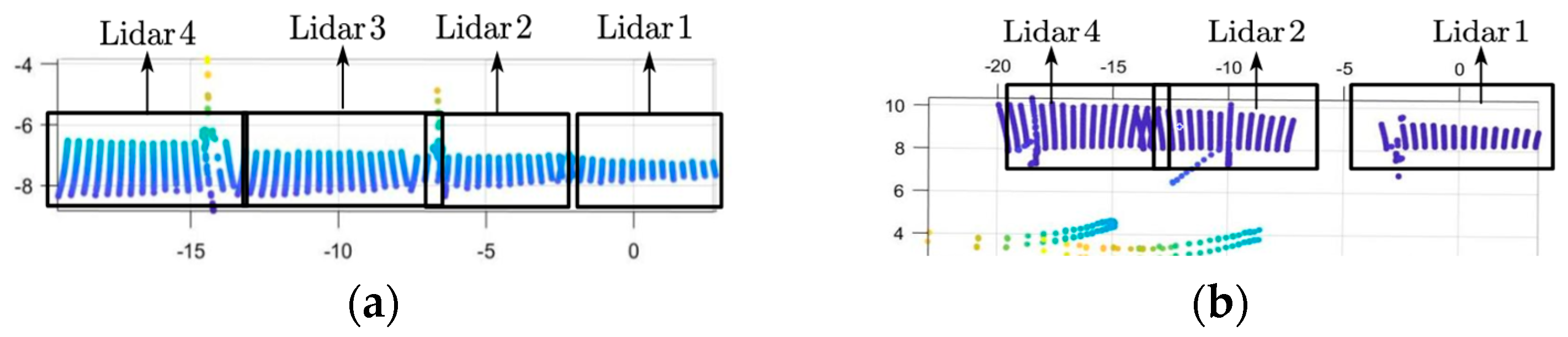
After completing multi-radar registration, we located the blade’s range of motion based on the magnitude of applied force. Subsequently, we applied direct-pass filtering [27] to the point cloud data that did not meet the requirements in the specified dimension direction. Background point clouds were removed and the level of data processing was reduced with satisfying efficiency. The results are shown in Figure 9.

The point cloud processed by the aforementioned method is formed into a new sample space, M1. The M1 point cloud data basically cover the edge appearance of the blade, but due to static loading cables and the occlusion of blade clamps, discrete point clouds remain, as shown in Figure 10. We can aggregate the point clouds that exhibit a certain pattern on the blade surface into a distinct category for subsequent processing. To process point cloud data, clustering algorithms such as k-means and DBSCAN are commonly used methods [28,29]. K-means is a distance-based algorithm that assigns a certain level of significance to all points, while DBSCAN is a density-based spatial clustering algorithm, where points in less denser regions are assigned lower weights (importance or influence) due to lower density in the perimeter. In the case of blades, we aimed for the discrete data of these specific points to have minor impact on the whole figure. Therefore, the DBSCAN algorithm proves more suitable for filtering out “the outliers”.

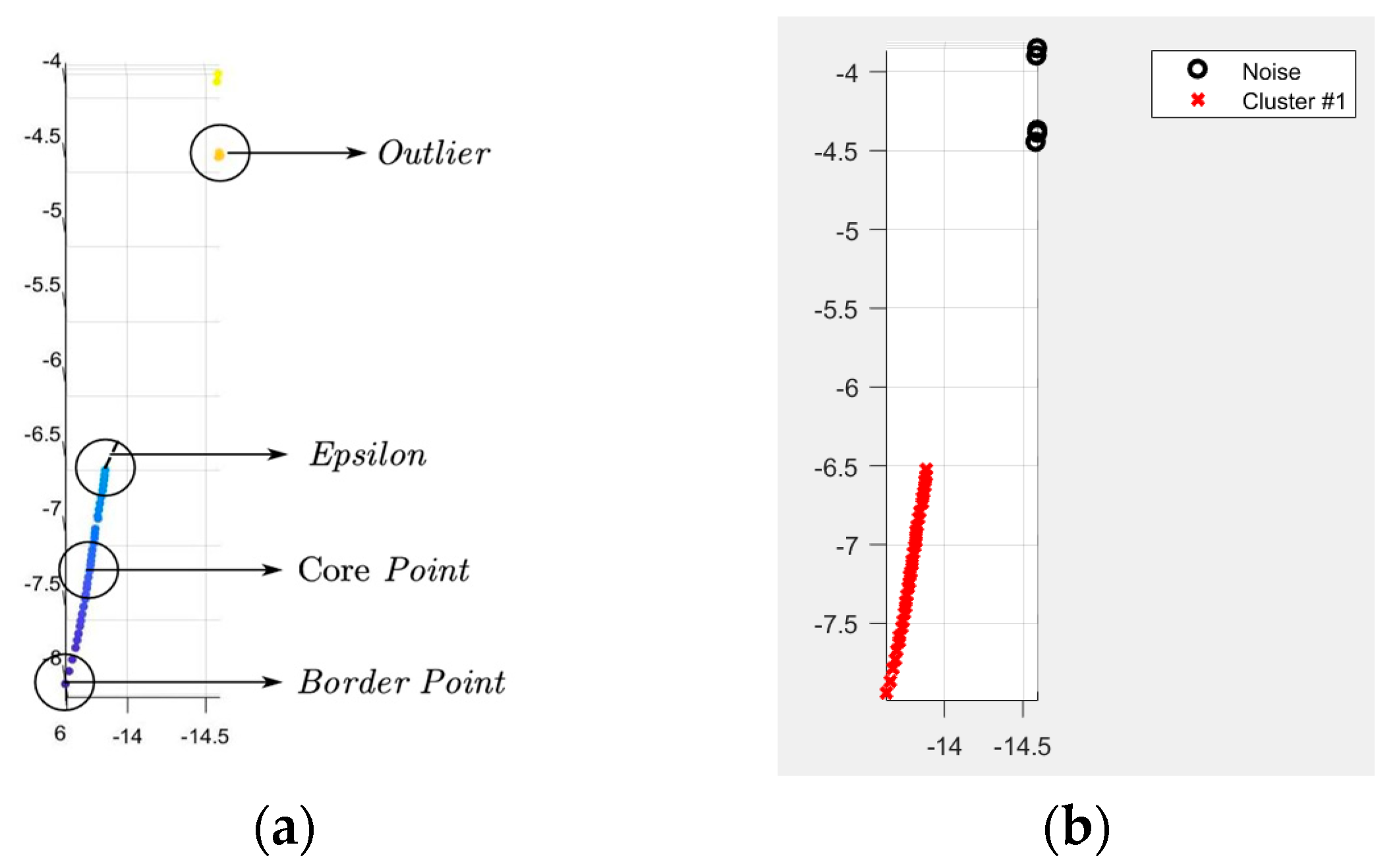
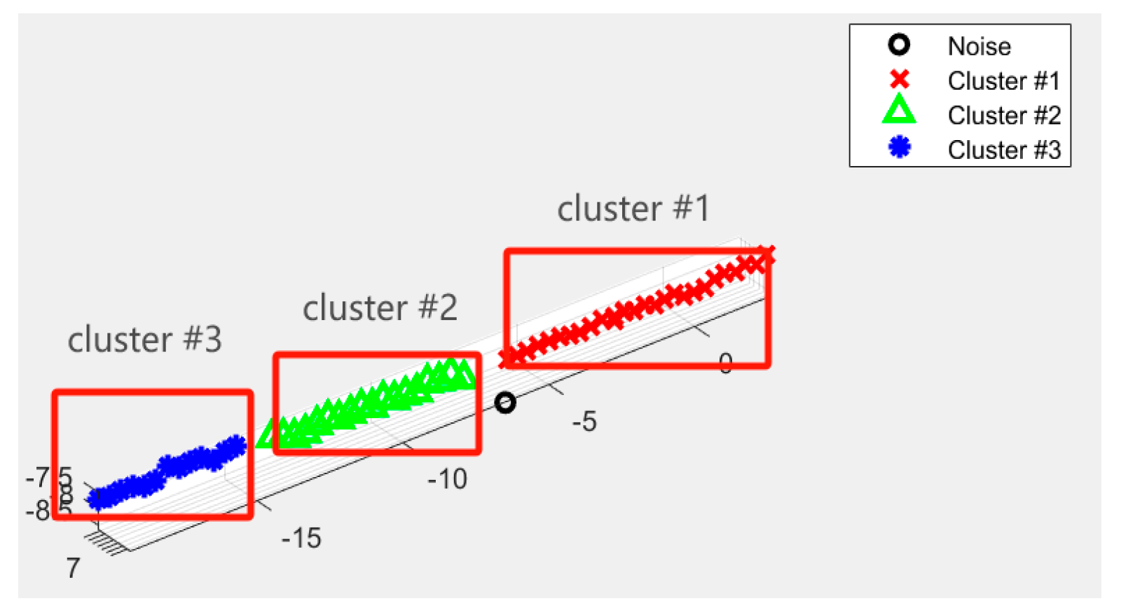
The DBSCAN algorithm divides regions with sufficiently high density into clusters of arbitrary shapes. Without knowing the number of clusters in advance, we can still identify the noise points sensitively. The algorithm mainly consists of two parameters, the neighborhood radius Eps and the minimum number of points Minpts, both of which help classify spatial points into core points, boundary points, and outlier points. For further explanation, let us select a random line of lidar data at a certain moment: we set Minpts to 4, and used Formula (9) to calculate the Euclidean distance Dist($p_i,p_j$) between each point $p_i(x_{p_i},y_{p_i},z_{p_i})$ and other points $p_j(x_{p_j},y_{p_j},z_{p_j})$ in the area. When the number of points inside that point’s corresponding radius Eps is greater than Minpts (the minimum number of points), this specific point is defined as a core point. Two core points with distances smaller than the neighborhood radius are density-connected. All density-connected core points and points within their neighborhood form a cluster. The results are shown in Figure 10.

$$\begin{array}{c}Dist\left(p_i,p_j\right)=\sqrt{{\left(x_{p_i}-x_{p_j}\right)}^2+{\left(y_{p_i}-y_{p_j}\right)}^2+{\left(z_{p_i}-z_{p_j}\right)}^2}\end{array}$$

(9)

In the traditional DBSCAN clustering algorithm, the output strongly depends on the parameter thresholds. When the threshold is too strictly selected, the same blade surface may easily be classified into multiple categories. Otherwise, discrete points may be regarded as part of the blade surface. Therefore, we proposed to update the neighborhood radius threshold dynamically based on the distance between the lidar and the blade surface.

At each moment, we calculated the mean of the point cloud M1 of the blade and recorded its distance to the lidar as d. We defined the maximum value during the entire static loading process as $d_{max}$, the minimum value as $d_{min}$, and used them to divide d into k intervals ($d_{min},d_{min}+{(d}_{max}-d_{min})/k$,$d_{min}+2({(d}_{max}-d_{min})/k)$,...,$d_{max}$). Each interval corresponds to a distinct value of Eps ($Eps1$, $Eps2$,...,$Epsn$). Minpts is set to a fixed value. The value of Eps is determined by the lidar resolution α, the right boundary of its corresponding interval, the minimum number of points Minpts, the constant β, and the coefficient μ, where μ is greater than 1, as shown in Formula (10):

$$\begin{array}{c}{Eps}_{\mathrm{i}}=\mathrm{\mu }\times \tan \left(\mathrm{\alpha }\right)\times \mathrm{Minpts}\times d+\mathrm{\beta }\end{array}$$

(10)

The filtering results are shown in Figure 11.

2.3. Spatial Line Clustering Algorithm

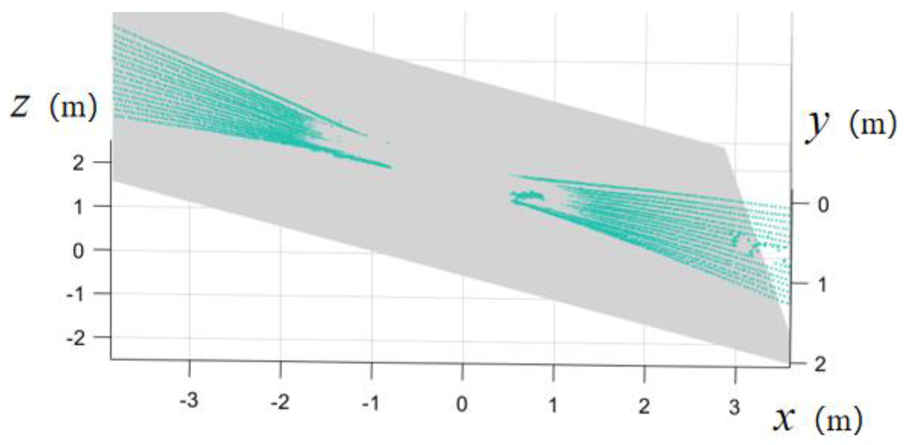
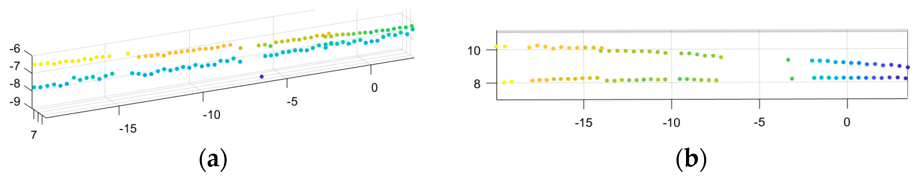
The extreme value of each lidar line is extracted to form a new sample space M2, as shown in Figure 12. In order to redress the errors generated during registration and recompense possible hardware problems related to the lidar, such as packet loss based on the UDP transmission protocol, which results in incomplete profile data of the blade surface, we suggested the spatial line clustering algorithm.

The main idea of this algorithm is integration after classification. By taking a contour line in Figure 10a and applying the DBSCAN clustering algorithm to divide it into k clusters, as shown in Figure 13, the noise points are removed directly. The coordinates of the cluster’s center point are used to represent its location. The point cloud set of any cluster is $Q=\left\{a_i\right|i=1,...,m\}$, where the coordinates of $a_i$ are ($a_{i,x},a_{i,y}$,$a_{i,z})$. Then, for the center point coordinates $P_k{(p}_{k,x}$,$p_{k,y}$,$p_{k,z})$ of Q, the calculation Formula (11) is as follows:

$$\begin{array}{c}{p}_{k,u}=\frac{1}{m}{\displaystyle \sum _{i=1}^m}{a}_{i,u}\left(u=x,y,z\right)\end{array}$$

(11)

In sequence, we performed curve fitting on the various clusters and defined $L_j$ as the fitting line of each cluster. Formulas (12) and (13) then calculate the distance $DisP2L(P_k,L_j)$ from the center point $P_k$ of other clusters to the curve and use it as an element of the adjacency matrix [30] Collections that are closer together are then recorded.

$$\begin{array}{c}{D}_{kj}=\left\{\begin{array}{c}\begin{array}{c}DisP2L\left(p_k,L_j\right),{k\ne j}_{ǁ}\\ 0,k=j\end{array}\end{array}\right.\end{array}$$

(12)

$$\begin{array}{c}{n}_j=\left\{P_k|k=\mathrm{1,2},\dots ,m\&DisP2L\left(P_k,L_j\right)<D\right\}\end{array}$$

(13)

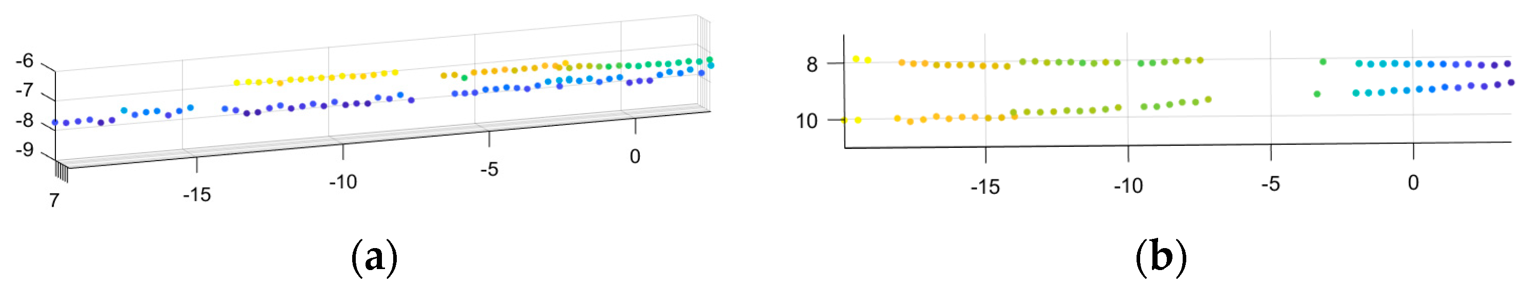
We found the combination with the most elements in $n_j$, $\mathit{max}\left(\left|n_i\right|,i=1,\dots ,m\right)$, and recorded it as $n_k$. We retained the elements in $n_k$ and deleted the remaining abnormal clusters that are not in the line clustering results, as shown in Figure 14.

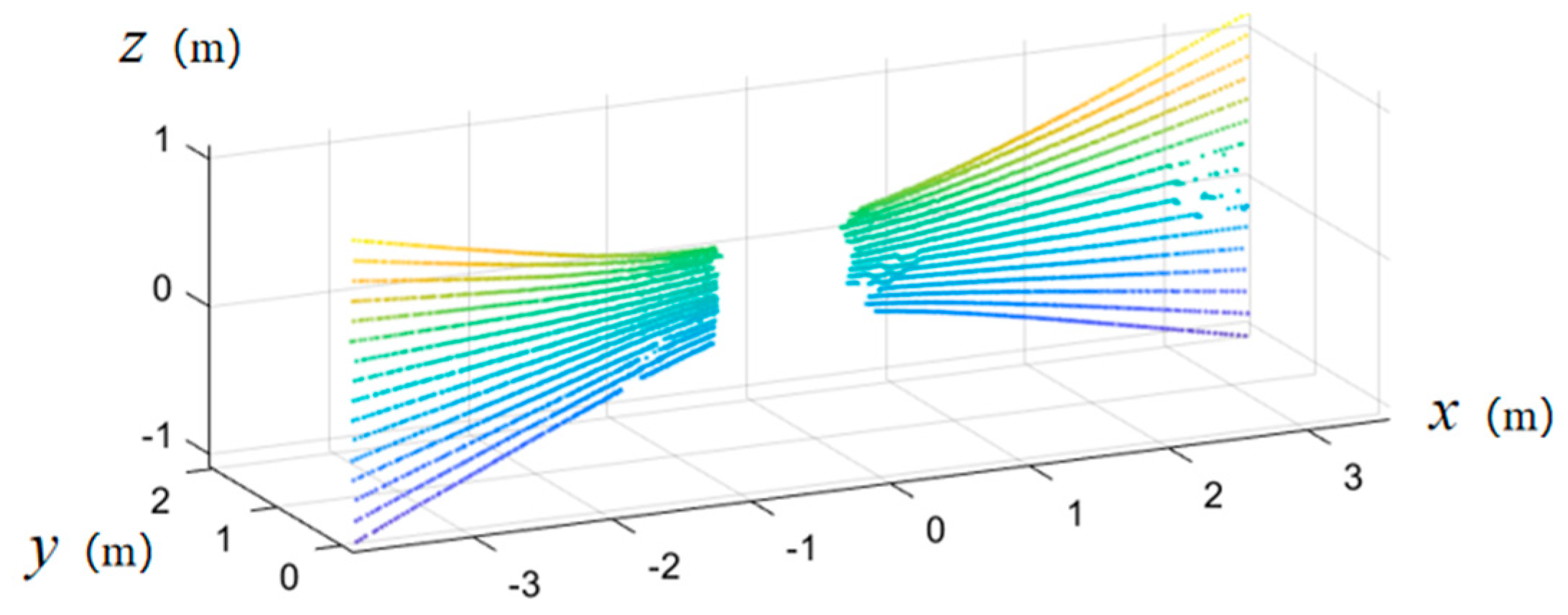
2.4. Space Line Integral

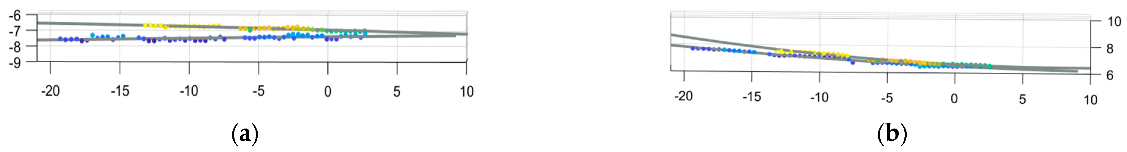
By observing the shape of the blade outline in Figure 3b, when static loading is performed in the oscillation direction, the yoz plane contour of the world coordinate system can be fitted to a linear Equation (14), and the xoz plane can be fitted to a quadratic Equation (14), as shown in Figure 15 and Figure 16:

$$\begin{array}{c}\left\{\begin{array}{c}\begin{array}{c}x=x\left(t^2,t\right)\\ y=y\left(t\right)\\ z=t\end{array}\end{array}\right.\end{array}$$

(14)

Generally, fitted space curves are less likely to be intersected. To “construct” this point of intersection, we selected a plane as a replacement, formed by the two axes with the largest deformation, onto which the intersection point is projected. This provides us with two of the coordinates. The remaining coordinates are determined by the mean of the projected point upon the two fitted lines. 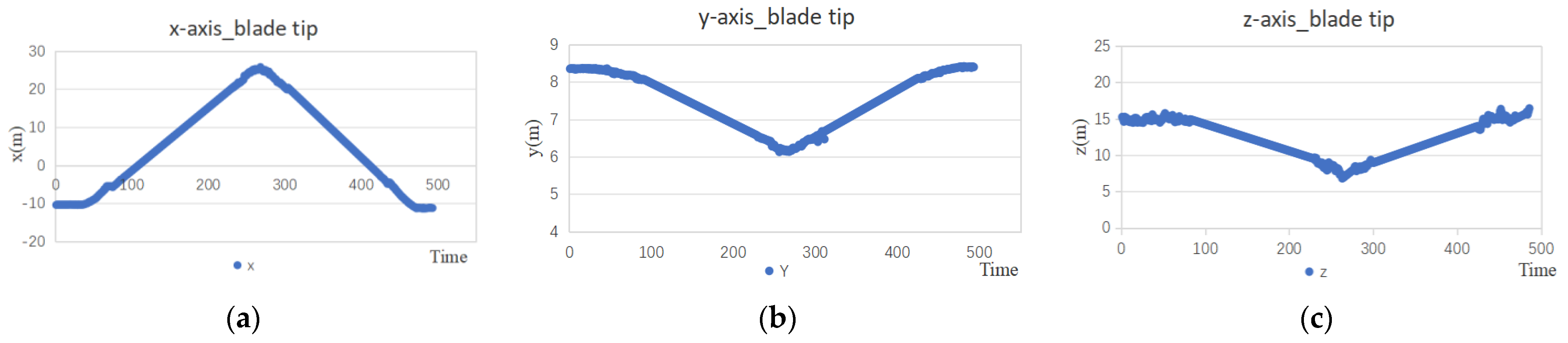During the process of static loading, the loading force is perpendicular to the blade axis, while deformation along that axis direction can be ignored, as shown in the dotted area in Figure 17. Therefore, the line integral value along the contour of the exhibition plane between the blade tip and the measured can be regarded as fixed.

In the curve integrals of the first type, when the integrated function equals 1, the physical quantity it represents is the curve’s length, as shown in Formula (15). Under initial stress-free conditions, we calculated and recorded the line integral of the blade’s contour from the measured point to the blade tip. 3D coordinates of the measured point are then calculated by combining the position of the blade tip at each moment, utilizing the fixed value of the line integral in this situation:

$$\begin{array}{c}\mathrm{L}={\int }_{\mathrm{\tau }}1\mathrm{d}\mathrm{s}=\underset{\mathrm{\alpha }}{\overset{\mathrm{\beta }}{\int }}\sqrt{{{[\mathrm{x}}^{\prime }\left(\mathrm{t}\right)]}^2+{{[\mathrm{y}}^{\prime }\left(\mathrm{t}\right)]}^2+{{[\mathrm{z}}^{\prime }\left(\mathrm{t}\right)]}^2}\mathrm{dt}\end{array}$$

(15)

3. Measurement and Analysis

3.1. Measurement System Composition

A lidar-based spatial large deflection measurement system is easy to install and has high accuracy. The hardware system comprises several key components, including: (1) multiple lidars, (2) lidar mounting bracket, (3) power supply module, (4) POE converter, (5) switch, (6) host computer, and several network cables, as shown in Figure 18.

3.2. Analysis of Measurement Results

Through the above steps, we obtained the 3D coordinates of the measured points at each time. Taking the blade tip as an example, the results are shown in Figure 19. The abscissa corresponds to time, while the ordinate illustrates the variations along the x-, y-, and z-axes of the blade in the world coordinate system.

Minimum oscillation direction test:

Table 1. Changes in 3D coordinates of different sections in the minimum oscillation direction.

z (m)	x-Axis Variation (m)	y-Axis Variation (m)	Total Variation of 3D Coordinates (m)
84	3.28	0.52	3.318
100	4.989	0.72	5.04
Leaf-tip 110	6.07	0.71	6.112

displays the 3D coordinate changes of three measured points at the initial and 100% loading moments in the minimum oscillation direction experiment.

Using the theoretical value T as a reference, we calculated the error of the measured value M obtained from the pull-wire sensor and the lidar at 84 m, 100 m, and 110 m of the blade, respectively, as shown in

Table 2. Comparison of cross-section errors of different methods in the minimum oscillation direction.

z (m)	Deformation—Wire Sensor (mm)	Deformation— Theoretical Calculation (mm)	Deformation— Lidar (mm)	Error—Wire Sensor and Theoretical Value	Error—Lidar and Theoretical Value
84	3094	3273	3318	−5.47%	1.37%
100	4731	4921	5040	−3.86%	2.42%
Blade tip 110	5561	6002	6112	−7.35%	1.83%

. Formula (16) shows the error calculation method:

$$\begin{array}{c}\mathrm{Error}=\frac{M-T}{T}\times 100\%\end{array}$$

(16)

Results’ analysis: The test results in the minimum oscillation direction are shown in Figure 20. The trends of the pull-wire sensor measurement values, theoretical calculation values, and lidar measurement values are consistent. Compared to the theoretical value, the measurement errors of the pull-wire sensor are −5.47%, −3.86%, −7.35%, and the lidar measurement errors are 1.37%, 2.42%, and 1.83% respectively. Clearly, the lidar measurement errors are all within 3%, outperforming the pull-wire sensor.

Maximum swing direction test:

In the maximum swing direction test, the lidar was placed in the loading stroke. When the blade moved directly above the lidar, the scanned point cloud formed the xoz plane. We removed this part from the calculation results. Since the static loading motion of the blade is consistent, we adopted interpolation fitting to supplement it. Results at the blade tip are shown in Figure 21. The abscissa corresponds to time, while the ordinate illustrates the variations along the x-, y-, and z-axes of the blade in the world coordinate system.

Table 3. Changes in 3D coordinates of different cross-sections in the maximum swing direction.

z (m)	x-Axis Variation (m)	y-Axis Variation (m)	z-Axis Variation (m)	Total Variation of 3D Coordinates (m)
84	17.77	1.39	2.70	18.03
100	28.96	1.88	6.49	29.74
Leaf-tip 110	35.29	2.21	8.32	36.32

shows the 3D coordinate changes of three measured points at the initial and 100% loading moments in the maximum swing direction experiment.

In the maximum swing direction test, the 3D coordinate changes of the measured points in Figure 21 have a similar trend with the results of the minimum oscillation direction test in Figure 19. This proves that the lidar measurement system is effective and can be extended to other testing processes.

4. Conclusions and Outlook

In light of the challenges posed by the commonly used pull-wire sensor measurement method in blade testing, including single dimensionality, significant errors, and high installation complexity, we proposed a simple, cost-effective spatial large deflection measurement system for wind turbine blades with multiple lidars. It can obtain the 3D information of any fixed point at any time and in any position without physical contact. Experimentally validated, in the minimum oscillation direction test, the measurement error is controlled within 3% compared to the theoretical value. Simultaneously, in the maximum swing direction test, the 3D coordinates of the measured point remain consistent with the changing trend observed under small deformation. These results confirm the feasibility of the system and its potential to be generalized.

The proposed system can be easily applied to the deformation measurement of other large structures (such as bridges, aircraft wings, etc.) and also used for amplitude measurements in fatigue testing of wind turbine blades. The system has wide practical value. However, the system still has room for improvement. On the one hand, we are studying the integration of the system to enhance its real-time capability. On the other hand, in response to the limitations of the multi-lidar point cloud registration method and the imperfect experimental settings, we are conducting in-depth research and making improvements. These efforts aim to further enhance measurement precision and enable the 3D reconstruction of blades using the lidar measurement system.