Volumetric Calibration Refinement of a Multi-Camera System Based on Tomographic Reconstruction of Particle Images

Abstract

The calibration of a multi-camera system for volumetric measurements is a basic requirement of reliable 3D measurements and object tracking. In order to refine the precision of the mapping functions, a new, tomographic reconstruction-based approach is presented. The method is suitable for Volumetric Particle Image Velocimetry (PIV), where small particles, drops or bubbles are illuminated and precise 3D position tracking or velocimetry is applied. The technique is based on the 2D cross-correlation of original images of particles with regions from a back projection of a tomographic reconstruction of the particles. The off-set of the peaks in the correlation maps represent disparities, which are used to correct the mapping functions for each sensor plane in an iterative procedure. For validation and practical applicability of the method, a sensitivity analysis has been performed using a synthetic data set followed by the application of the technique on Tomo-PIV measurements of a jet-flow. The results show that initial large disparities could be corrected to an average of below 0.1 pixels during the refinement steps, which drastically improves reconstruction quality and improves measurement accuracy and reliability.

1. Introduction

Volumetric measurement based on distributed multi-camera systems requires a proper calibration. Typical methods to calibrate the system include the estimation of the parameters of the lenses and image sensor positions in the form of a mapping matrix, which is based on the parametric description of the imaging in the form of a pinhole camera model where the parameters were gained from imaging a calibration target (objects with known size and position in space). With the presence of distortions or glass walls in the optical paths, the pinhole model may be superseded with polynomial mapping functions. Such a model is the third order polynomial camera model [1], which is used to describe the mapping function. The inverse of these equations can be used to compute the lines of sight (LOSs) originating from each pixel in each camera. Even though a precise calibration is done initially, an unintentional movement of one or more cameras later in the experiments can introduce biases [2,3]. This is especially important in voxel-based reconstructions of particle-filled volumes, as the reconstruction quality of the particles largely depends on the calibration accuracy. Such biases especially deteriorate the results of volumetric velocimetry measurements such as 3D Particle Tracking (3D-PTV) or Tomographic PIV (Tomo-PIV) [4]. A general review of Particle Image Velocimetry is given in [5]. These 3D methods have been become more and more popular in experimental fluid mechanics in the last decade, as the camera hardware, as well as the computing power for image processing, have been rising continuously. The increasing engineering interest in 3D measurements in fluid dynamics also manifests in the application of X-ray tomography [6], 3D PTV in granular packings [7], 3D PTV with digital holography [8] and 3D PTV for near-wall flows [9]. In addition, tracking algorithms have improved using different variants of matching strategies with the help of tomographic reconstruction [10]. To improve the calibration process, the method of self-calibration was introduced [11] which uses particle images to enhance an initial camera calibration. The procedure segments the observed volume into smaller sub-volumes in which the particle locations are triangulated. Disparities are then calculated based on their distance away from the theoretical crossing of the epipolar lines in the image plane and those are used to correct the initial calibrations. Arroyo and Hinsch [2] recommended for Tomo-PIV to reduce the remaining disparities in the calibration setup to a minimum of 0.4 pixels. This also depends on the spatial resolution, the number of cameras, the viewing angles and the pixel noise. Therefore, any calibration refinement procedure must aim to minimize disparities in the image planes of all cameras.

The present work represents an alternative approach introduced in 2018 [12], which uses iterative voxel-field reconstructions and back-projections to calculate the disparity maps, reducing the remaining disparity below 0.1 px. It is based on the tomographic reconstruction of the particles themselves and the comparison of their back-projections with the original images using 2D cross-correlation. Therefore, particles are reconstructed using MART or SMART algorithms (see e.g., [13,14]) and small sub-volumes of the full volume are then back-projected to the image planes and cross-correlated with the local image pattern in the original images. The offset of the peak from the center in the correlation map represents the local disparity. Multiple realizations of calibration records are used to eliminate the influence of ghost particles and noise on the final results. The whole process is called Volumetric Calibration Refinement (VCR). The present work provides detailed simulations of the influencing parameters and an experimental verification of the performance of the method.

In the following, we consider without restriction of generality the simplified case of a typical three-camera arrangement, useful for volumetric velocity measurement, e.g., 3D particle tracking (3D-PTV) or tomographic PIV (Tomo-PIV) (see Figure 1). It is assumed that the three cameras are arranged in the same horizontal x-z-plane (cam #1,2,3: β = 0°) but with different viewing angles (α₁ = −45°, α₂ = 0°, α₃ = +45°) (see also the data given in

Table A1. Camera settings for methodological simulations.

	Cam #1	Cam #2	Cam #3	Cam #4
Camera size full width × height (px)	250 × 250	250 × 250	250 × 250
Camera alpha α	α1 = −45°	α2 = 0°	α3 = +45°
Camera beta β	β1 = 0°	β2 = 0°	β3 = 0°
Camera pixel size (µm)	10	10	10
Magnification (mm/vx)	1/10	1/10	1/10
pixel to voxel ratio	1	1	1
Lens configuration	Ideal telecentric	Ideal telecentric	Ideal telecentric
Initial mapping function	Ideal rectilinear	Ideal rectilinear	Ideal rectilinear
Initial camera error translational	Δpx = +3	-	-
Initial camera error rotational	Δγ1 = 0°	-	-
Refined mapping and LOS equation	3rd order X,Y 2nd order Z	3rd order X,Y 2nd order Z	3rd order X,Y 2nd order Z

in Appendix A). The projection of a particle from the world coordinate system into the image plane is described mathematically for each camera via its mapping functions—see the equations given in Appendix B. The coefficients of the mapping functions are typically computed from calibration images of known objects whose world coordinates are predetermined in the volume. Together with the inverse of the mapping functions, which is the calculation of the LOSs for each pixel in each camera, the computation of tomographic reconstructions using MART or SMART algorithms are carried out [14] (see Appendix B). The particles are reconstructed as contiguous clusters of voxels, ideally; the center of gravity is intersected by all the LOSs that originate from the particle image centers in the image planes. Since the particle images are finite in size, the reconstruction is always a spheroidal composite of cohesive voxels representing the particle. However, if larger deviations of the mapping functions from the actual optical conditions occur, the voxel cluster is deformed and the position of maximum intensity is dislocated from the error-free situation. The proposed method aims to correct the disparities in the image planes (and therefore the mapping functions) such that the LOSs intersect again and the spherical character of the particles is fully restored.

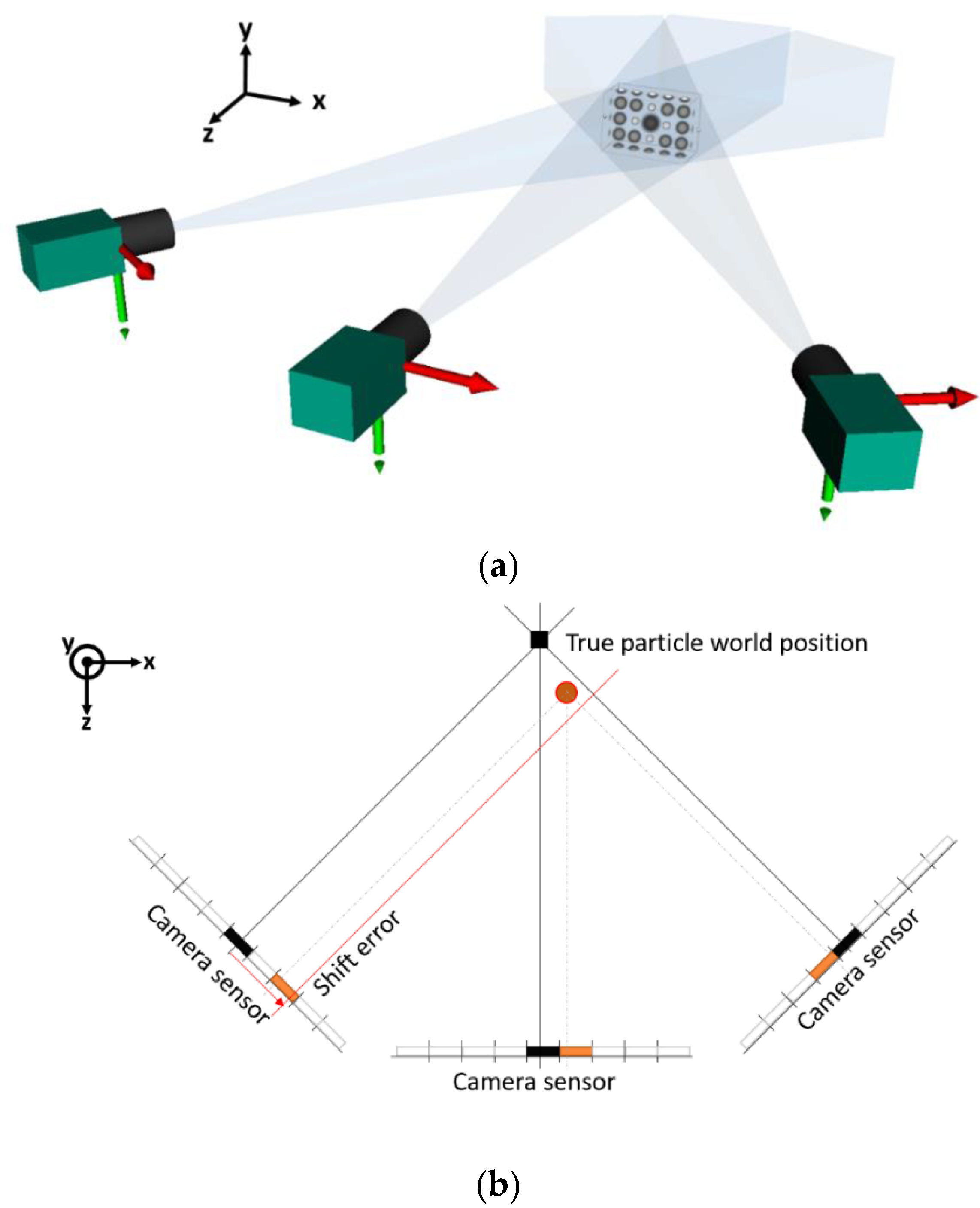
2. Methodology of Calibration Refinement

The working principle is exemplarily illustrated for the simplified case of the three-camera setup shown in Figure 1. We further assume that the imaging system should be such that all LOSs are rectilinear and perpendicular to the sensor plane (telecentric approximation). The gray solid lines in Figure 1b show the LOSs’ origination from the particle image centers for perfect calibration, intersecting at the center of gravity in the true particle world coordinate. A virtual misalignment of the leftmost camera is introduced in the form of a shift in the sensor plane (along its horizontal axis in the sensor plane). This results in a shift to a new 3D center position of the voxel cluster (red circle) offset from the original position. The diameter dP of the particle image in the image plane is the reason that a compact intensity cluster can still be generated in the voxel space. Possible corrections for this situation are the adaptation of the mapping function in various ways: on the one hand, the mapping functions for cam #1 can be corrected so that this camera is virtually moved back to its original position; for the present case, the accumulated disparity vector would be the inverse of the red arrow shown in Figure 1b to correct for the initial misalignment of cam #1. On the other hand, the mapping functions could be corrected for all cameras simultaneously, resulting in a situation represented by the black dashed lines. Note that both corrections lead to a perfect reconstruction of the particle. In the latter case, however, the world coordinate system defined with the particle location is shifted relative to the cameras.

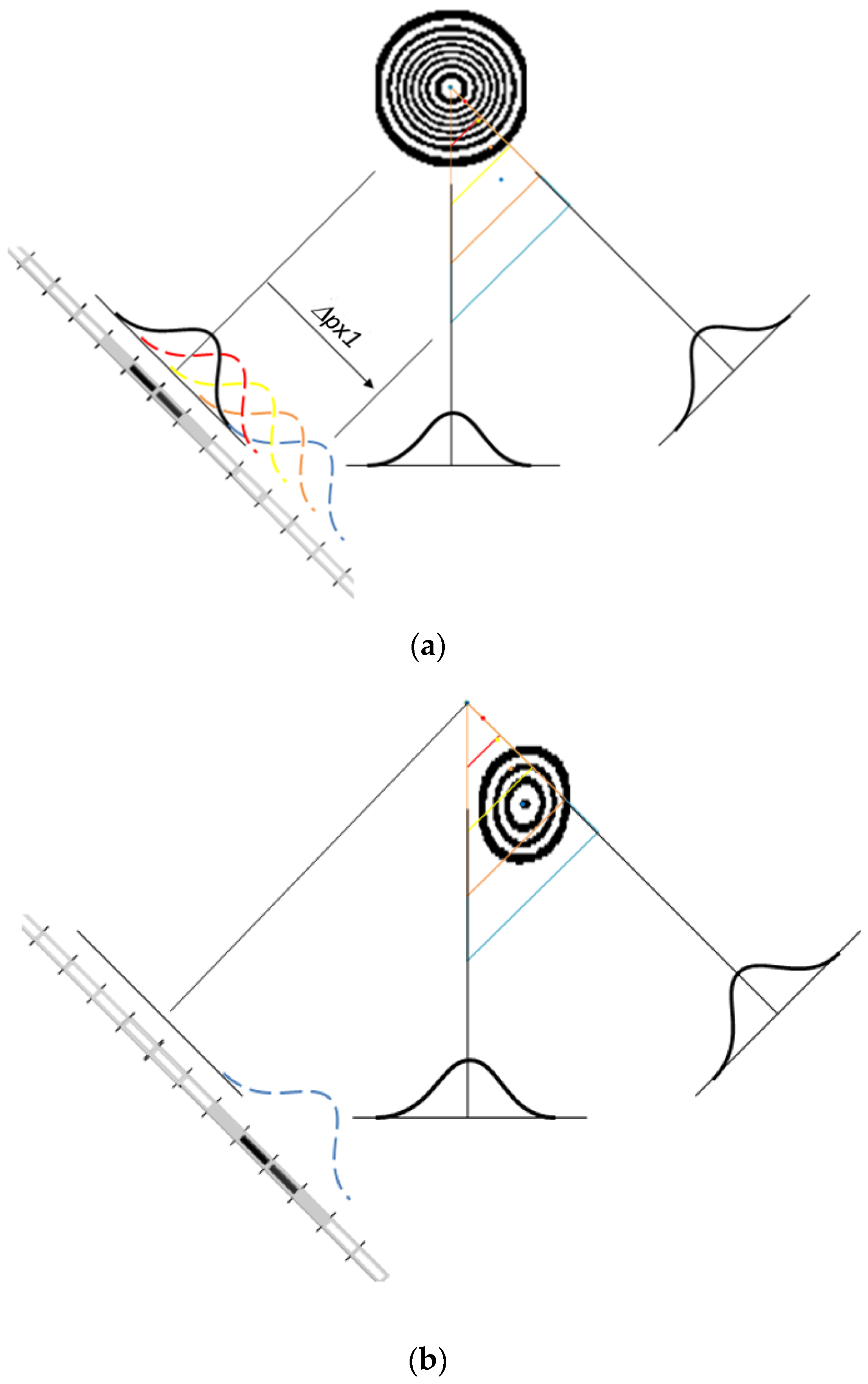
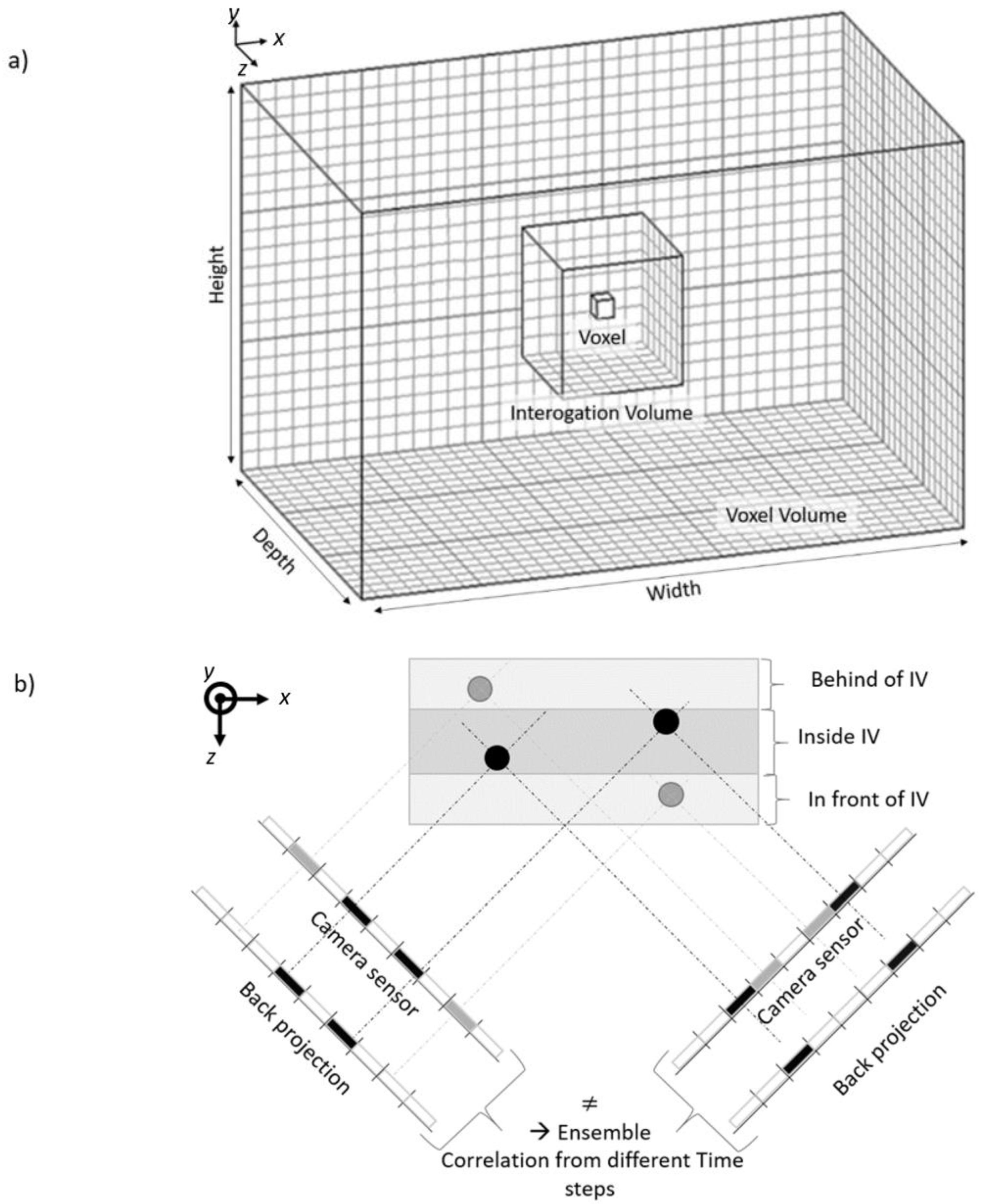
2.1. The Shape of a Particle Reconstruction with Camera Mismatch

The characteristic feature used in our method herein is the fact that—even in case of a mismatch—the Gaussian intensity profile of the disk-like original particle images preserves a spheroidal structure in the tomographic reconstruction and, furthermore, the back-projections of those reconstructions generate particle images with near-Gaussian intensity profiles again (along the major axes of the contour). This holds as long as the disparities are smaller than about half the particle diameter dP. A simulation of a synthetic Gaussian blob of an $e^{-2}$ diameter of D = 30 vx in a voxel volume represents the situation of a 10-times super-resolved image of a typical tracer particle in the image plane. The intensity at the voxel position vx (i,j,k) = (X_vx,Y_vx,Z_vx) with a distance $r\le D/2$ to the center of the blob at (X₀,Y₀,Z₀) is calculated according to the following equation:

$$I(v{x}_{i.j.k})=I_{max}·e^{(-2\frac{r^2}{D^2/4})}$$

(1)

where

$$r^2={(X_{vx}-X_0)}^2+{(Y_{vx}-Y_0)}^2+{(Z_{vx}-Z_0)}^2$$

(2)

The intensity distribution of the blob is mapped onto the cameras planes (magnification M = 1, perfect linear mapping functions equivalent to rectilinear parallel LOSs), leading to a particle image with a diameter of dP = 30 px with good spatial resolution to recover the details of the Gaussian intensity distribution of the original blob. From those images, the blob is again reconstructed using MART. The LOS calculation and the MART reconstruction follows the method of Kühne (2011) (see Appendix B). In all reconstructions, we use 10 iterations with a relaxation factor μ = 1. This represents the error-free reference situation. Then we shift the image in the left cam #1 stepwise to introduce a calibration error and reconstruct the voxel volume again. The result given in Figure 2 is shown in the horizontal median plane of the reconstruction. To emphasize the shape of the intensity distribution and the location of the intensity maximum, the images are represented as contours of constant intensity with constant incremental value.

In the case of a perfect calibration (zero mismatch), the reconstructed blob has a spherical structure (circular in plan view) with a Gaussian intensity distribution, the maximum located at the geometric intersection of the LOSs, originating from the intensity centers of the particle images. When the left camera cam #1 is shifted to the right by an increasing number of pixels, this reconstruction increasingly deforms into an elliptical shape, shifting the intensity maximum further from the original center (see Figure 2b). Meanwhile, the location of maximum intensity always remains in the inner part of the triangle defined by the particles center LOSs. The limit of a successful reconstruction is a maximum displacement of the cam #1 on the order of ¾ of dP, at which a compact spheroidal contour can still be seen. The character of the Gaussian intensity distribution in the back-projections along the major axes of the particles is preserved to this extent of dislocation. This allows us to use sub-pixel analysis in the 2D cross-correlation procedure during the correction step documented in the next paragraph.

2.2. Cross-Correlation of Original Images with Back-Projected Images

The correction is based on the comparison of the original image and the back-projection using the method of 2D cross-correlation. The peak in the correlation map provides the local shift-vector (disparity) between the center of the back-projected particle image relative to the representation of the particle in the original image. As the disparity might vary over the field of view, the procedure is done stepwise in small interrogation volumes (IVs), distributed in a 3D grid over the whole volume of interest, see Figure 3. Each IV is projected back into the image plane of all cameras. In the original images, interrogation windows (IWs) are built of a size and location that correspond to the back-projection of the IV centers and box corners into the image plane. The IWs are then 2D cross-correlated with the projections of the IVs and the resulting correlation maps are stored. The offset of the peak location relative to the center is then searched in the map to determine the disparity. Due to the contribution of images of particles behind or in front of the IV, the correlation map is affected by random noise, which increases with increasing volume depth and particle number density. This random contribution is reduced by ensemble averaging the maps of different snapshots (or different IV in case the disparity is constant, e.g., if the cameras undergo only translational vibrations).

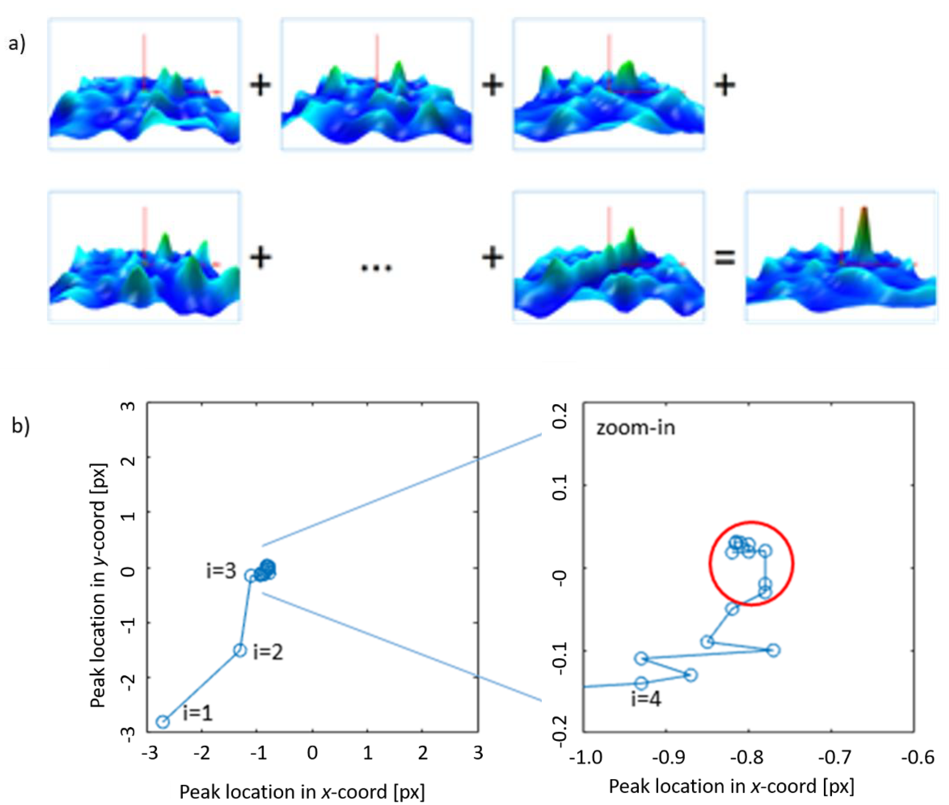
2.3. Ensemble Averaging of Correlation Maps from Snapshots

The typical procedure is to repeat several realizations of the calibration experiments (snapshots of statistically independent locations of the particles in the different realizations) and add the corresponding correlation maps at each IV (Figure 4). Alternatively, in case the disparity is constant, e.g., if the mismatch is due to translational vibrations of the cameras, the correlation maps of each IV can be added to each other, which requires only a single snapshot. By using this method, the random noise decreases and the peak is elevated against the background, which is known in another context as Ensemble Correlation [15]. As the image content is based on distributed Gaussian disks (the particle images), the peak location in the summed-up 2D correlation maps can be calculated with subpixel accuracy using a 2-D Gaussian fit of the peak. The importance of the ensemble averaging of the correlation maps is highlighted in the plot of the peak location for the example shown in Figure 1. The initial correlation map of a single IV (i = 1) in the series shows a dislocation of approximately −3 px in the x-direction and −3 px in the y-direction (see Figure 4b left), which is not physical at the given imposed mismatch for cam #1. After averaging of three maps, the peak is at −1.1 in the x-direction and remains within a radius of 0.3 px for all further iterations. From the 10th iteration onwards, the position fluctuates around a position of −0.8 in the x-direction and 0.0 px in the y-direction with a deviation of less than 0.05 px (see the red circle in Figure 4b (right)). This is an example of a fully converged solution and represents the local disparity which might be used for the initial correction. As shown later, the magnitude of this correction step depends on the particle density.

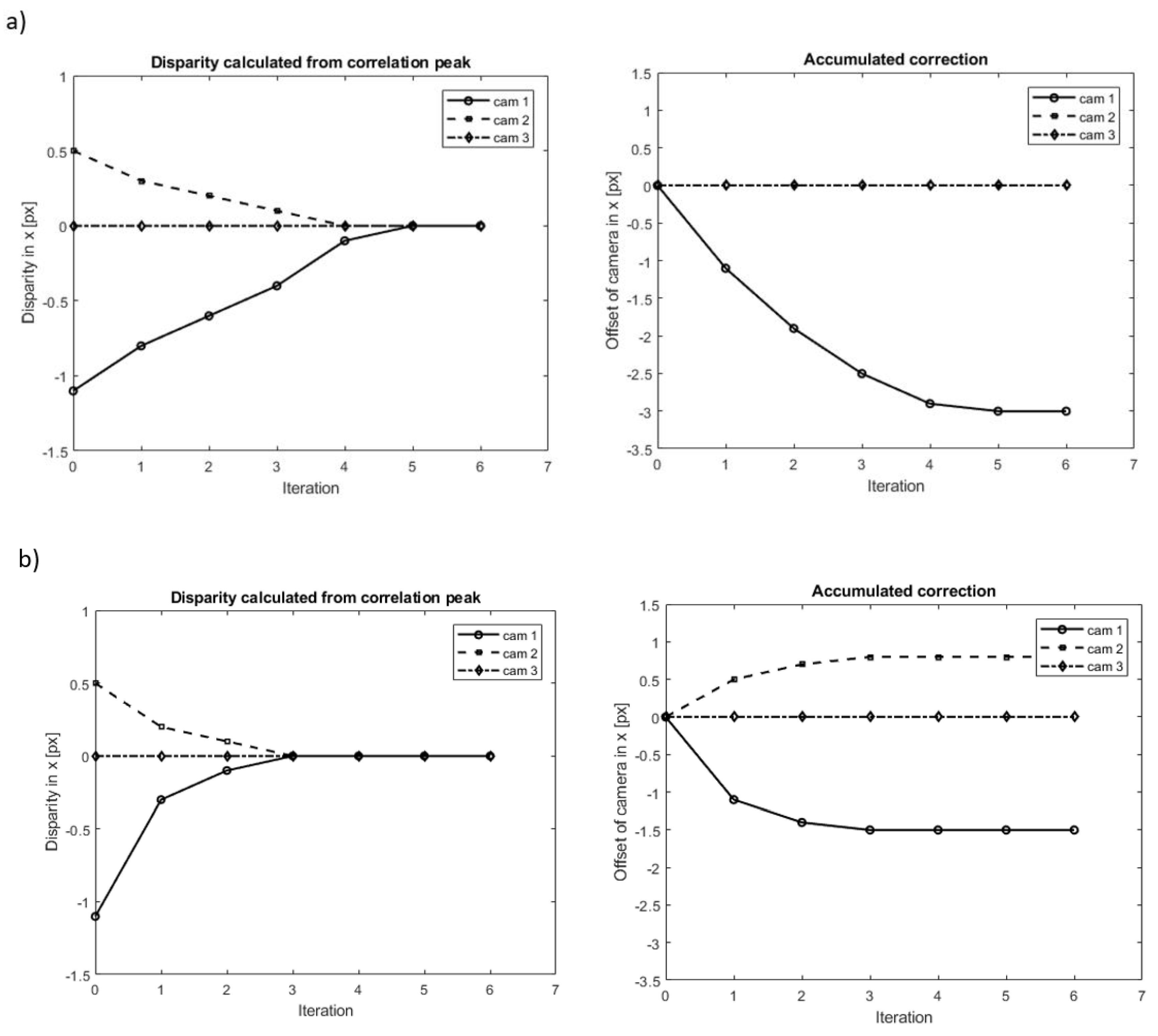
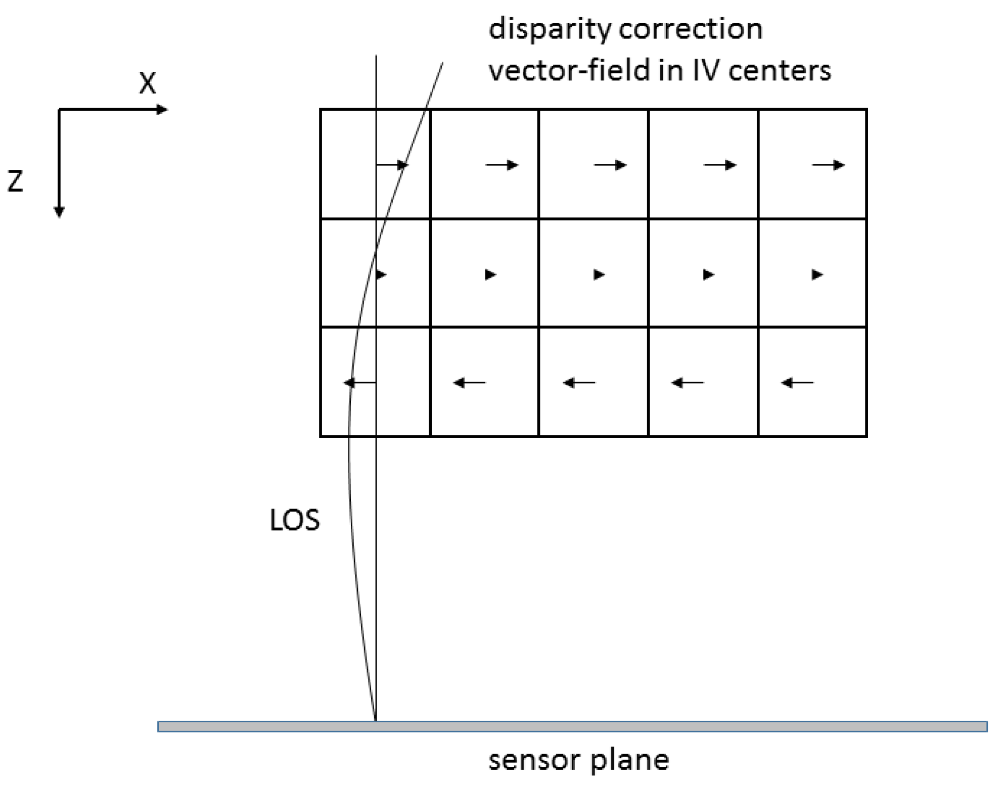
2.4. Correction Steps

Step 1: The initial voxel reconstruction is subdivided into a 3D grid of overlapping cubic voxel clusters of finite size (called interrogation volumes (IVs)). Alternatively, the volume reconstruction can be done in a piecewise fashion for all the IVs individually, which, however, is not very efficient. This subsampling addresses the fact that the correction might not be uniform across the entire volume. As the corrections affect the coefficients of the mapping functions and those are polynomials of second order in the direction of the depth, the recommended number of IV in the depth-direction along the Z-axis should be at least three. Correspondingly, the number along the X- and Y-axis should be minimum four for the third order polynomials in the image plane. Therefore, the number of IV in the voxel volume should be at least a 4 × 4 × 3 grid of IV. This ensures that the spatial resolution and size of the interrogation volume (IV) are adapted to possible gradients in the disparity field. Ultimately, the disparity field is assumed to be a smoothly varying function in all three directions.

Step 2: Perform the cross-correlation with the original image and the back-projected images (with masking of all intensity information outside of the IV).

Step 3: Repeat the Steps 1–2 for an ensemble of calibration images, taken from different snapshots (only one single snapshot is necessary in case the disparity is constant in the field, e.g., for simple translational mismatch). Store the correlation maps for each center location of the pack-projected IV in the image planes for all cameras and add all correlation maps of the ensemble. A sufficiently large number of snapshots needs to be taken to ensure that a sufficient number of ensembles with particles inside the IV contribute to the summation process (again, only a single snapshot is required if the disparity is constant in the field, the summation is then done with the maps of the different IVs). If you choose a denser grid and smaller size of IV as the one recommended in Step 1, more calibration images are required but this is no general shortcoming of the method proposed.

Step 4: Finally, locate the peak position in the ensemble-averaged maps with sub-pixel accuracy and store these disparities for each position in the image plane that corresponds to the back-projected center of the IVs. This is done for all camera views. The disparities are not to be understood as the total deviation between initial calibration and fully error-free calibration. Rather, they indicate in which direction and by what amount a first step for the correction of the mapping functions should be taken. Therefore, we name these shift-vectors in the following correction steps for the given iteration.

Step 5: Use a least-squares method to find the new parameter of the mapping functions from the additional disparities in the image plane for each center of IV (see Appendix B). Calculate the new LOSs and compute a new tomographic reconstruction with the updated mapping functions. As we use polynomial mapping functions, the refinement takes into account gradients in the correction field that may be caused by camera rotation or more complex mismatch.

Repeat Step 1–5 until the residual (average of all cameras, or max. of all cameras) between two successive correction steps is below a pre-defined level, in the following we chose 0.1 px.

2.5. Typical Iterative Correction Performance

To illustrate the correction performance, we consider the example of an error in the mapping function, which is due to a change of the camera position (between initial calibration and measurement situation) and needs a refinement of the mapping functions to get back to an “ideal” error-free situation. Therefore, particle images in the original images (later called “zero-shifted images” in the simulation) do not match with the back-projections, as those are affected by using the wrong mapping functions in the MART reconstruction (in the simulation, this is done by introducing a “shift” mismatch on one camera in the MART, equivalent to changing a linear parameter in the mapping function of this camera). In a real laboratory environment, the “zero-shifted images” are the original images taken for the calibration refinement. The back-projections are affected by inaccuracies in the mapping functions and therefore the particle images in the back-projection and the original images do not exactly overlap. This is what we correct in the refinement method by changing the mapping functions until both overlap ideally. Synthetic particle fields are generated to test the convergence of the iterative procedure, applied to the simplified situation at Figure 1b. A thick voxel sheet (depth 160 vx, width 225 vx, height 11 vx) is generated and filled randomly with Gaussian blobs of diameter D = 3 vx to generate particle images with a density of 0.001 ppp. The acronym “ppp“ stands for particles per pixel area, which is typically used to describe the source density on the sensor plane depending on the number density of the particles in the 3D volume. The 2D area consumption of the projection of the particles is the dominant parameter determining the source density in the image plane. If this is too high because of a too large number of particles, the particle images tend to overlap. All centers of the particles lie in the horizontal mid plane at a height of 6 vx. The initial mapping functions are linear in the X,Y, and Z-directions, which assumes straight parallel LOS normal to the image planes (telecentric conditions) at a magnification of M = 1 without any optical distortion. First, the equations for the LOSs are determined and the corresponding images of the camera setup are generated by back-projection (see Appendix B). The ground truth is then the MART reconstruction from these images. In a second step, a shift is introduced on cam #1, as indicated in Figure 1b, and a new voxel volume is computed based on this mismatch. Finally, the correction procedure is started by back-projection of the masked IVs and cross-correlation is done with the IWs in the original (zero-shifted) images. The same procedure can be repeated with different random arrangements of particles in the voxel sheet such that 10 correlation maps exist for each IV, which then are used for the ensemble average.

Figure 5 shows the iterative correction procedure if only cam #1 with the largest disparity is corrected after each correction step (a) compared to the situation with all cameras corrected (b) simultaneous. Convergence for the first case is reached after five correction steps while the simultaneous correction already leads to an error-free situation after three iterations. As a side effect of the latter method, a shift of the Z-location of the measurement domain can happen, which has been discussed in another context by Cornic et al. [16]. The performance of the refinement process can be seen by comparing a top-view image of the MART reconstruction in the 11 vx thick sheet before correction and after correction (only cam 1) (see Figure 6). The number of ghosts is largely reduced and the shape of the particles gets more homogeneous and circular. The benefit of lower ghost level intensities for Tomo-PIV has been discussed, for instance, by Novara et al. in 2010 [17] and de Silva et al. [18]. In general, those ghost particles are typically generated in tomographic reconstructions of particle fields as a consequence of multiple crossings of LOSs. Therefore clusters of voxels are not only reconstructed at the true particle position but sometimes also in a smaller cluster nearby the original particle. A discussion of the influence of ghost particles was given in [19].

Further performance tests are done with the same three-camera configuration (error-shift on cam 1 of +3 px in the x-direction and correction of this camera only) to investigate the influencing parameter and their importance for stable convergence. As performance criteria, we give the initial correction shift and the number of iterations until we reach a residual of less than 0.1 px relative to the error-free situation, remaining under this level for any further iteration. To better represent an experimental environment, one of the parameters is random noise, added to the images. After the particles are placed on the simulated image, the entire image is added with white noise; this is comparable to the real situation since it affects also the images of the particles. Typical conditions are zero-average white noise with a gaussian variance σ = 0.01, and a mean = 2 σ for images in the gray-level range [0, 255]. As the typical procedure for self-calibration is image pre-processing to reduce those noise levels, we do the same herein and use a local average salt and pepper filter and a final Gaussian smoothing with a 3 × 3 kernel. Thereafter, a tomographic MART procedure (10 iterations and a dampening factor of 1) re-computes the voxel volume from these images. These volumes are then the ground truth, including possible ghosts and noise.

The results given in

Table 1. Parameter study of performance sensitivity to particle density, angular displacement and noise level for a three-camera arrangement in the same plane as defined in Table A1 and Appendix A.

Particle Density ppp	Angular Displacement of Cam #1 and Cam #3	Noise Level Variance	Initial Correction Step of Cam 1 (from +3 px Error-Shift)	Minimum Number of Ensemble Additions to Achieve Peak Position within 0.1 px Radius	Iterations to Correct Cam #1 Down to 0.1 px Offset
0.001	±45°	0	−1.1	4	5
0.003	±45°	0	−1.0	6	7
0.005	±45°	0	−0.8	10	9
0.008	±45°	0	−0.4	20	13
0.010	±45°	0	−0.3	22	-
0.001	±22°	0	−0.6	4	10
0.001	±45°	0.00	−1.1	3	5
0.001	±45°	0.01	−0.6	6	7
0.001	±45°	0.02	−0.5	10	10
0.001	±45°	0.03	−0.6	20	-

show that the correction procedure still works with larger levels of noise at a variance σ = 0.02 and for particle densities as high as 0.008 ppp. Beyond that, the final residual starts to oscillate with amplitudes larger than 0.1 px around the error-free situation and therefore convergence is not achieved. This does not mean that the refinement is not successful, as the error after 10 iterations remains below an offset < 0.2 px. Another important factor is the angular displacement of the cameras. As expected, a larger angular displacement improves the performance, as the tomographic reconstruction of the particles is generated from a wider field of angular views and therefore the particles are represented more as spherical voxel clusters. Decreasing the angles leads to a stiffer behavior (more iterations are necessary) of the correction process because of the increasing tendency towards elongated shapes of the reconstructed clusters. Recalling that with smaller angular displacement the reconstructions get elongated in viewing direction, therefore the voxel space is filled with more voxels, which increases the tendency of ghosts. Regarding particle densities and noise levels for the lower angular displacement of 22°, the general trend remains the same; the results deteriorate with higher particle densities and higher noise levels. Therefore, we do not add additional data for this case in Table 1.

2.6. Treating Larger Mismatch with Image Pre-Processing Using Gaussian Blur

We assume a very large mismatch of cam #1, which is larger than the particle image diameter dP of a single particle. Without further processing of the original images, no tomographic reconstruction of the particle would be possible. In order to deal with this situation, the images can be pre-processed with a Gaussian blur so that the particle diameter dP is artificially enlarged. The larger the diameter of the kernel, or the more often the kernel is applied to the image successively, the higher the probability to successfully reconstruct a first, rough representation of the particle in the voxel space. However, as this enlargement of the particle diameter also introduces a higher probability of ghosts, it should only be applied to the first correction step and selecting only the brightest particles in all camera views. The processing is done in a hierarchical manner, starting with artificially enlarging the particle images in all camera views via image pre-processing (e.g., blurring with a Gaussian 5 × 5 px kernel). The first correction typically leads to a 50% reduction in the average disparity, which then offers to reduce the blur kernel size stepwise and using more particle images, until ending with using the original images in the further iterations. This will provide maximum accuracy without affecting the quality of the reconstructed particles in the final result.

3. Numerical Assessment

A synthetic four-camera cross type configuration is considered as a more general case of camera arrangement (and possible dislocation in different planes) (see Appendix A,

Table A2. Camera settings for parametric simulations.

	Cam #1	Cam #2	Cam #3	Cam #4
Camera size full width × height (px)	800 × 500	800 × 500	800 × 500	800 × 500
Camera alpha α	α1 = 0°	α2 = +45°	α3 = 0°	α4 = −45°
Camera beta β	β1 = −45°	β2 = 0°	β3 = +45°	Β4 = 0°
Camera pixel size (µm)	10	10	10
Magnification (mm/vx)	1/10	1/10	1/10	1/10
pixel to voxel ratio	1	1	1	1
Lens configuration	Ideal pinhole	Ideal pinhole	Ideal pinhole	Ideal pinhole
Initial mapping function	Ideal rectilinear	Ideal rectilinear	Ideal rectilinear	Ideal rectilinear
Initial camera error translational (px)	Δpy = +5	Δpy = +5	Δpx = −3	Δpx = −3
Initial camera error rotational	Δγ1 = 0°	-	-	-
Refined mapping and LOS equation	3rd order X,Y 2nd order Z	3rd order X,Y 2nd order Z	3rd order X,Y 2nd order Z	3rd order X,Y 2nd order Z

). The performance of the VCR is tested for different seeding densities, particle image diameters dP and IV sizes to assess the capabilities of this method. In addition, synthetic data for a Hill-type velocity field are applied to move the particles in the voxel volume and investigate the performance of the VCR on the final velocity results of 3D PIV velocity fields. The cameras are in cross-type arrangement with ±45° angular displacement in the horizontal and vertical plane and have a distance of 610 mm from the volume center (X,Y,Z) = (0,0,0). They observe a simulated volume of 75 × 45 × 27 mm³ with a simulated camera resolution of 800 × 500 pixels on a 2/3 inch sensor at a magnification of 1:5. The length of one voxel equals 0.1 mm in physical space. The synthetic volume is filled randomly with Gaussian blobs of a given diameter D ($e^{-2}$ diameter) and number density to achieve a specified particle image diameter dP and ppp density. The initial mapping functions are linear functions in the X,Y, and Z-directions, simulating the situation of an ideal pinhole imaging system with no distortion (generated with the Soloff polynomials and the LOSs are calculated therefrom). The particle image diameter dP is directly proportional to D and is varied in this study by choosing different blob diameters. Initial images are generated from these voxel volumes by back-projection. Again, white noise is added to the images and thereafter image pre-processing is done (local salt and pepper filter and Gaussian smoothing with a 3 × 3 kernel). A tomographic MART procedure (10 iterations and a dampening factor of 1) re-computes the voxel volume from these images. These volumes are then the ground truth. All cameras are corrected simultaneously and the norm of all disparity vectors of all IV and all cameras is taken as an indicator of the overall performance of the system.

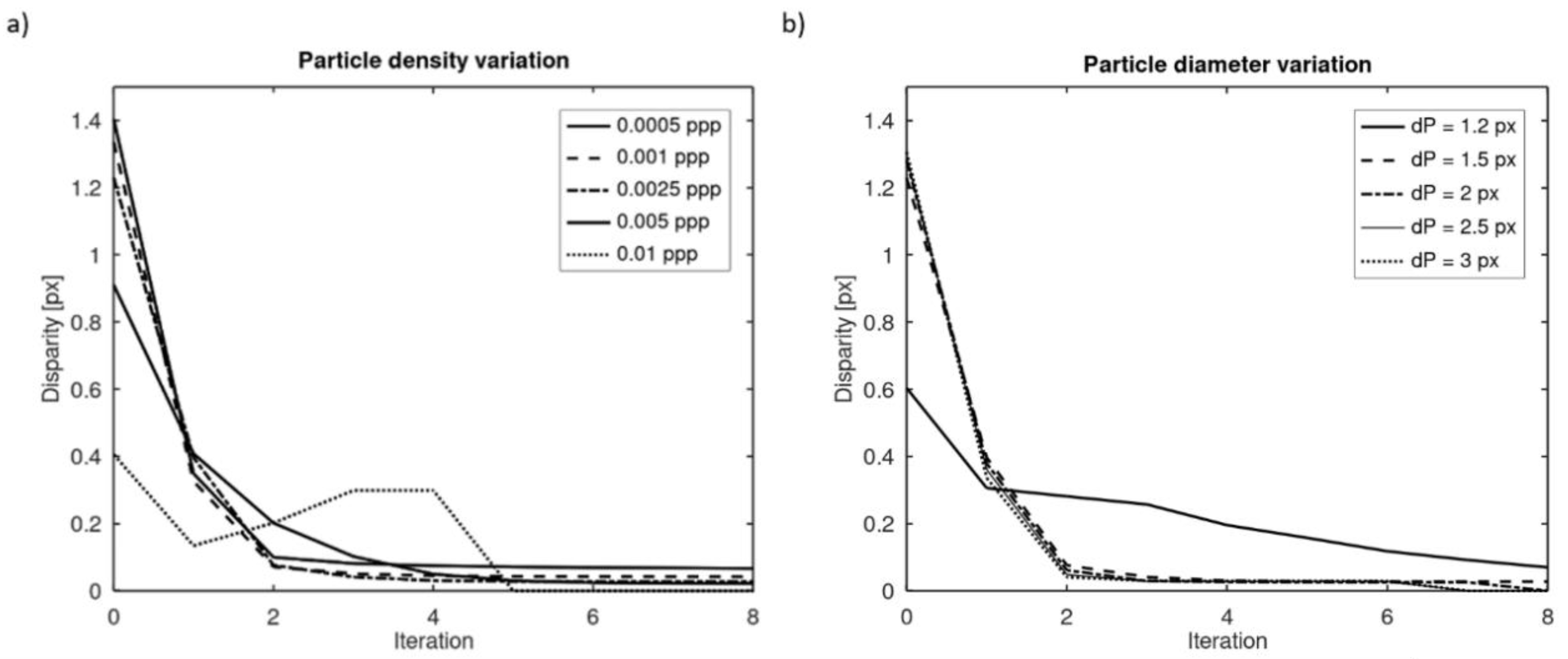
3.1. Influence of Particle Image Diameter and Seeding Density

The standard settings for the VCR in this case are image sets of five snapshots for each camera with a particle diameter of dP = 2 px at a seeding density of 0.0025 ppp, all generated with the above-described procedure. The total volume is subsampled in a mesh of cubic IVs with equidistant spacing in each direction such that the complete volume is covered. For a standard IV size of 80 × 80 × 80 vx, a set of 9 × 5 × 3 positions are generated. To introduce a possible calibration mismatch, cam #2 is moved for 0.4 mm in the y-direction (corresponding to a linear shift of 4 pixel). The calculated correction shift in cam #2 to reduce the initial mismatch in each iterative step is plotted in Figure 7 for the different parameters of particle image diameter (a), particle density (b), number of images for ensemble averaging (c) and interrogation volume size (d).

Figure 7a shows a re-configuration back towards a near error-free situation after four iterations for a particle diameter dP between 1.5 and 3 px. All final correction shifts show a residual in the range between 0.023 and 0.052 px. In comparison, for very small dP = 1.2 px, the refinement fails because of peak locking effects influencing the correction steps. At low seeding densities in the order of 0.001–0.0025 ppp, the correction is nearly complete with only a single image, once there are at least 1–2 particles in each of the IVs. The general rule is the more images that are used, the smaller the residual becomes (not shown here). Generally speaking, using three to five images for the ensemble averaging is a good compromise between computational costs and accuracy under these conditions. Also, the size of the interrogation volume has an influence on the process. Figure 7d shows that an IV size of 30 × 30 × 30 vx seems to be sufficient for the given seeding density of 0.0025 ppp; however, there is a risk of drop-out of particles in some of the IVs. The correction improves for larger IV sizes, though it reduces the spatial resolution. A typical size of 50 × 50 × 50 vx with five snapshots is a good compromise to also capture stronger gradients in the correction field.

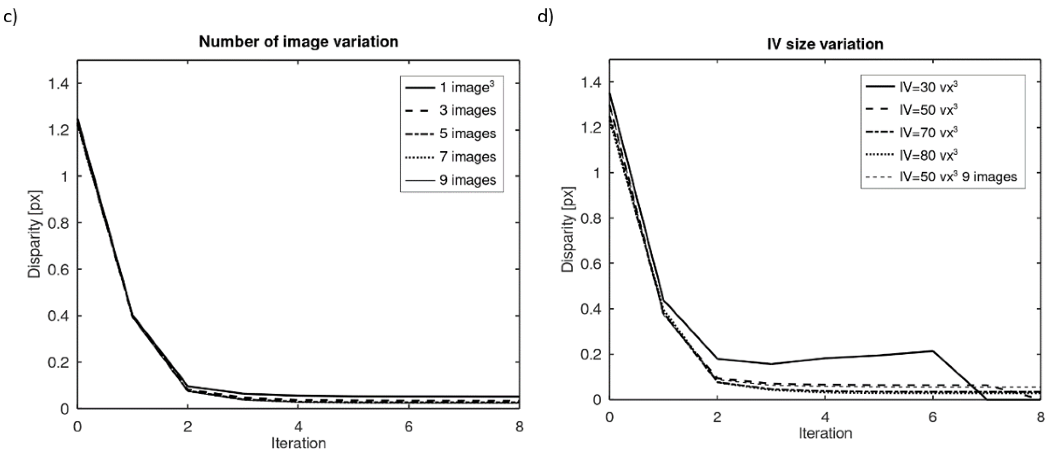
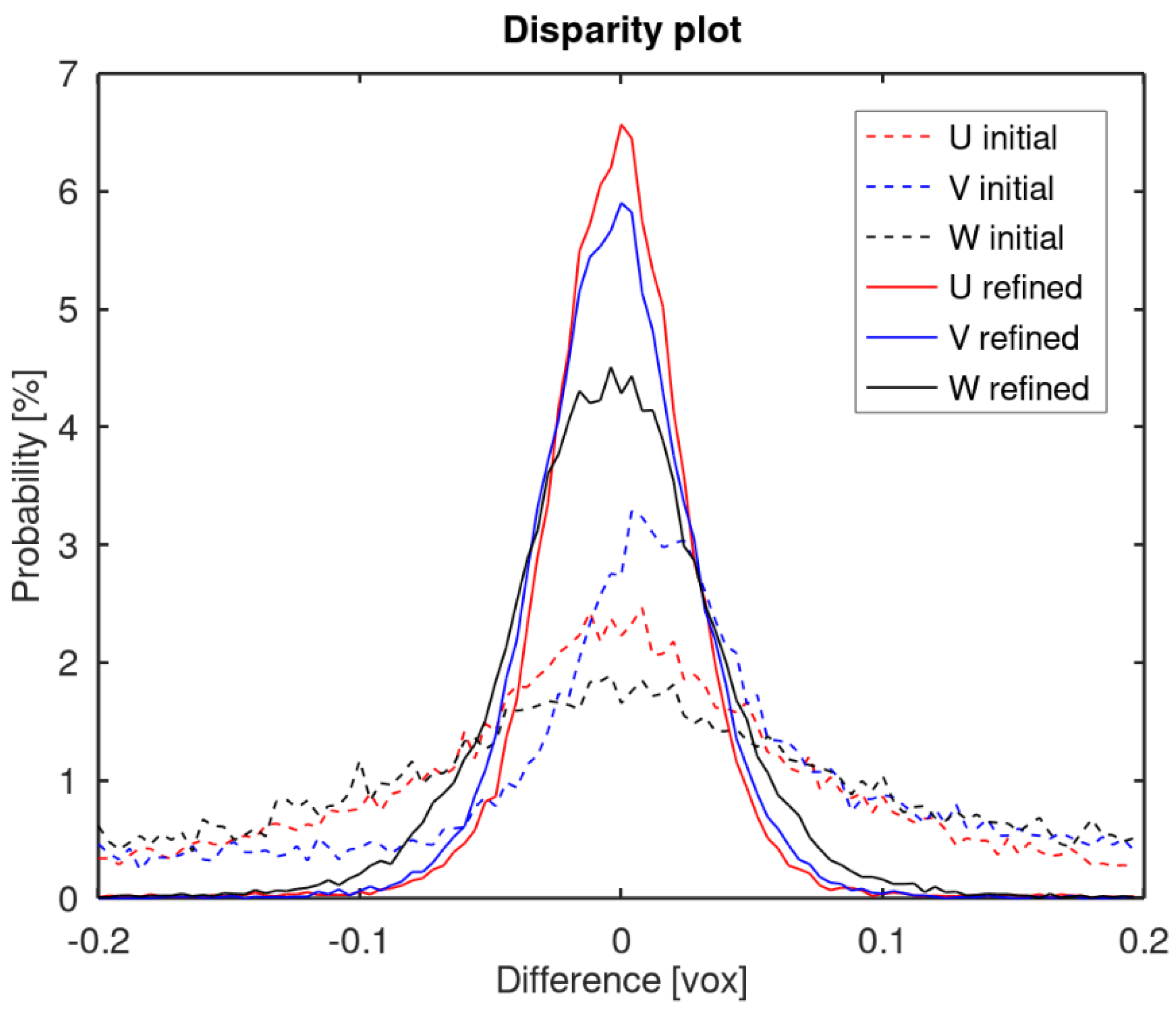
3.2. Influence of Errors on All Cameras

In a typical experimental environment, more than one camera may change its position. Therefore, in the second test, case errors are introduced in all four cameras. Relative to the error-free situation, the top and right cameras are moved up by 0.5 mm (five pixels). Similarly, the bottom and the left cameras are shifted 0.5 mm to the right (five pixels). This leads to a maximum potential calibration error of more than nine pixels. To tackle this possibly large disparity, all images are pre-processed initially with a Gaussian blur (5 × 5 kernel) as described in Section 2.6 and hierarchical processing with stepwise reduction of the kernel size in each iteration step is done (3 × 3 kernel in the second step; from the third step on the original images are used). A number of five snapshots are taken and the IVs have a size of 80 × 80 × 80 vx with a mesh resolution of 9 × 5 × 3 positions. For the refinement, all cameras are corrected simultaneously in each iteration step. The results (not shown here) demonstrate that, within four iterations, the average disparity drops from 1.5 pixel to well below 0.1 pixel. This performance is not much different from the previous one where the error mismatch was only introduced to one camera. In addition, it proves that the Gaussian blur offers to correct for larger disparities without loss in convergence.

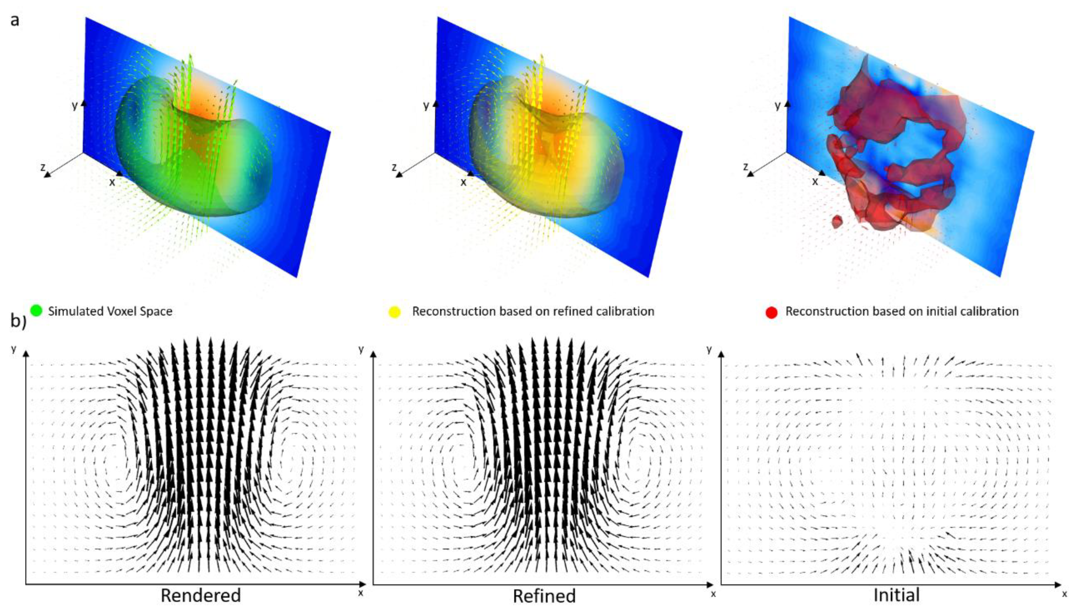
3.3. Performance Tests with Synthetic Velocity Data

Testing the full performance of this refinement method for 3D Velocimetry applications, voxel fields are generated with particles shifted over several time-steps. Gaussian blobs of D = 3 vx are displaced in the cartesian world coordinate system (X,Y,Z) according to a given steady flow field (Hill-type vortex of Radius R = 120 vx, see Appendix C and [20]). The simulation conditions are the same as in Section 3.1, Section 3.2 (see Appendix A, Table A2). The characteristic velocity U₀ of the vortex ring is adjusted such that the particle shift between successive timesteps corresponds to a displacement of 5 vx. The simulated flow is transferred into the observed-fixed reference system where the vortex is traveling from bottom to top with a velocity of U₀ and the outer velocity at infinity is zero. The synthetic voxel fields are filled with a higher seeding density, leading to typical particle image densities of about 0.045 ppp in the images. The initial and the refined calibrations described in Section 3.2 are used to reconstruct the voxel spaces back from the generated images. In a final step, pairs of voxel spaces are analyzed by 3D least squares matching (3D LSM, see Westfeld et al. [21], Maas et al. [22]) to generate the velocity vector maps of the Hill-type vortex (LSM conditions: cuboids of 30 × 30 × 30 voxel elements with a 50% overlap in all directions) (see Figure 8). The final result is a vector field of 51 × 31 × 19 vectors in the volume, transformed back into the right-handed Cartesian coordinate system (X,Y,Z) with the components (U,W,W). For VCR, the iso-surfaces of constant Q-criteria, a vortex detection method (see Hunt et al. [23]), shows a clear reconstruction of the vortex torus, which largely improved the results with the initial calibration (with the artificial camera mismatch). Figure 8b highlights the differences between the initial and refined calibration. The mismatch mainly affects the regions of higher velocity, which could not be reconstructed in the inner of the sphere.

The histograms of vector differences relative to the rendered case are plotted in Figure 9. The distributions are approximately symmetric to zero and similar to a Gaussian profile with the peak in the center. For the VCR results, less than 0.1% of all vectors show a deviation larger than 0.1 vx and the distribution has a smaller variance with a sharp peak. In comparison, one order of magnitude higher percentage of vectors (1%) show a deviation of more than 0.1 vx difference for the initial calibration. In addition, the statistical values also improve; for instance, the standard deviation changes from 0.04 vx in the case of the initial calibration down to 0.01 vx in the refined calibration.

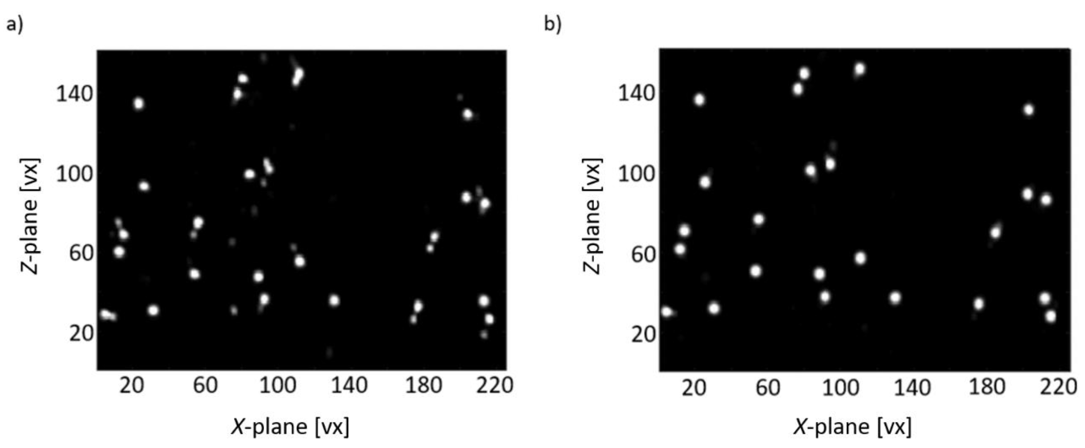
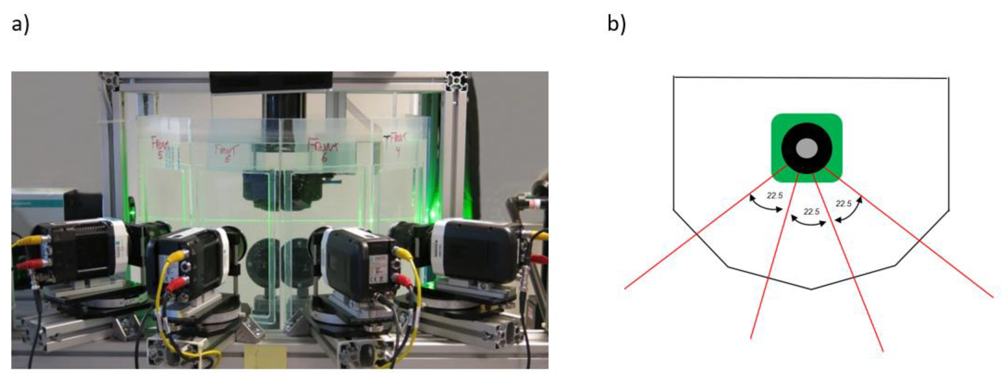
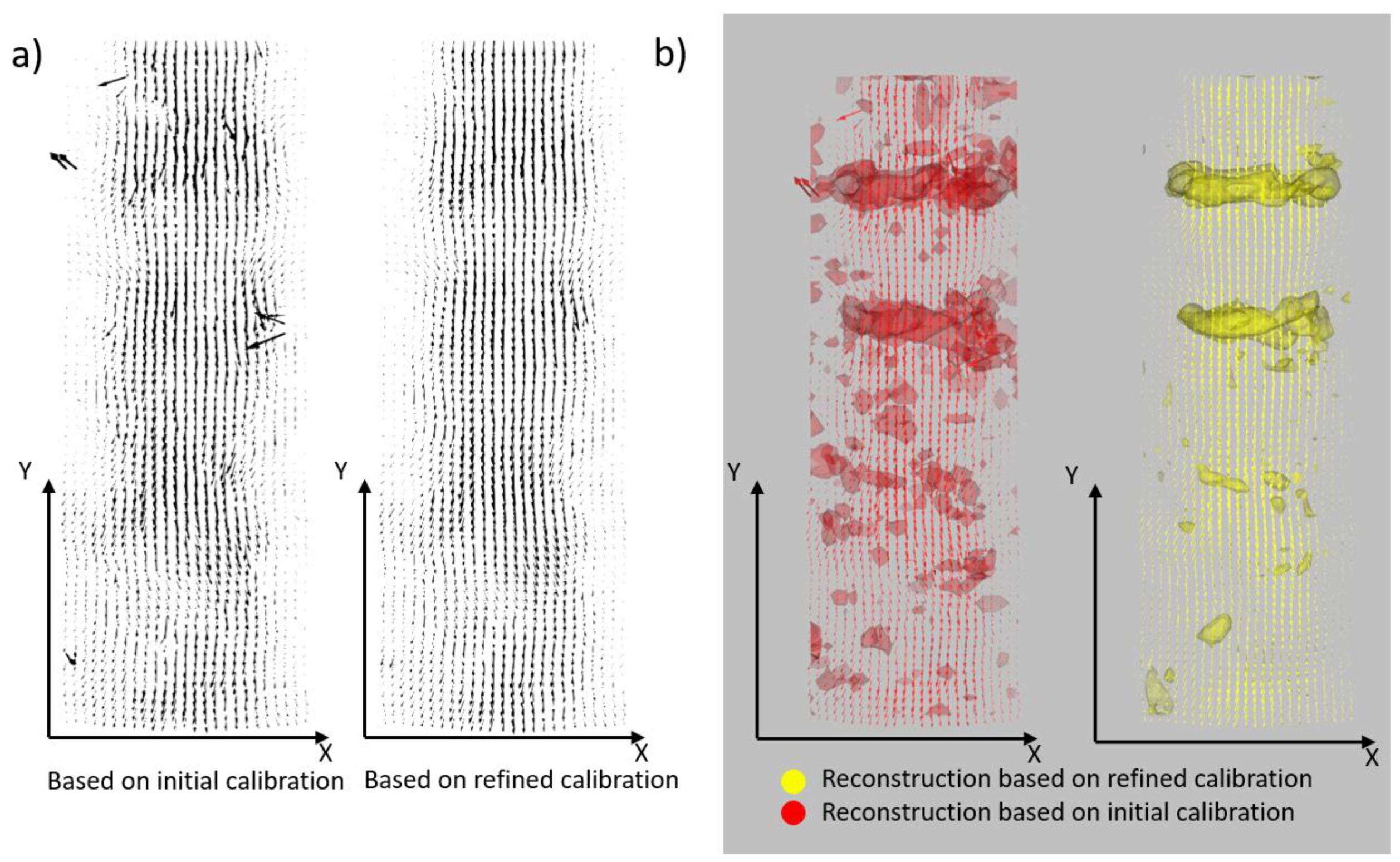
4. Performance Tests with Experimental Data

To verify that the method proposed in this paper is also suitable for real-world experiments, a 3D jet flow experiment was studied with Tomo-PIV. The flow was investigated in a small water tank with a polygonal cross-section (see Figure 10). The jet emits in vertical direction downwards from a nozzle (orifice diameter of 12.36 mm) submerged in the upper water level with. The jet velocity at the orifice was approximately U₀ = 0.23 m/s, resulting in a jet Reynolds-number of approximately 2830. Under these conditions, the jet was in the transitional regime, where large-scale vortical structures still dominate the flow field in 3–4 jet diameters down of the orifice. The flow was measured by a set of four Speed-Sense M 310 (1280 × 800 px) cameras in an in-line configuration (see

Table A3. Camera settings for experiments.

	Cam #1	Cam #2	Cam #3	Cam #4
Camera size full width × height (px)	1280 × 800	1280 × 800	1280 × 800	1280 × 800
Camera alpha α	α1 = −33.75°	α2 = −11.25°	α3 = 11.25°	α4 = 33.75°
Camera beta β	β1 = 0°	β2 = 0°	β3 = 0°	β4 = 0°
Camera pixel size (µm)	20	20	20	20
Magnification (mm/vx)	1/10	1/10	1/10	1/10
pixel to voxel ratio	1:1.1	1:1.1	1:1.1	1:1.1
Lens configuration	Zeiss 100 mm	Zeiss 100 mm	Zeiss 100 mm	Zeiss 100mm
Initial mapping function	Soloff	Soloff	Soloff	Soloff
Initial camera error translational	unknown	unknown	unknown	unknown
Initial camera error rotational	unknown	unknown	unknown	unknown
Refined mapping and LOS equation	3rd order X,Y 2nd order Z	3rd order X,Y 2nd order Z	3rd order X,Y 2nd order Z	3rd order X,Y 2nd order Z

in Appendix A). A DualPower 30–1000 Laser was used to illuminate a 10 mm thick light volume located along the middle of the tank in the vertical direction of the jet. This camera configuration yielded a resolution of approximately 15 px/mm. As tracer particles, hollow glass spheres (S-HGS-10 particles, Ø = 10 µm, Dantec Dynamics) were added to the water. In the following, we illustrate the improvement against the “standard” calibration often used in stereo PIV and Tomo-PIV is the so-called Soloff calibration method [1], where targets with known coordinates in 3D space are recorded. Herein the initial calibration was done with a dotted calibration target moving along the Z-axis and taking images at different positions. For the refinement step, it is possible to use either (a) extra particle recordings at lower particle density or (b) the original recordings for 3D PTV or Tomo-PIV with high particle density after filtering the images such that only the brightest particle images in all camera views remain. Herein, for refinement a set of five snapshots was taken with low particle density of 0.001 ppp. Then, the particle image density was increased to about 0.045 ppp and up to 4000 individual images were recorded with a repetition rate of 1 kHz for the Tomo-PIV processing. The raw images were processed by subtracting the background, performing a sliding minimum thresholding, and smoothing with a 3 × 3 Gaussian kernel.

A volume of 27 × 65 × 27 mm³ was reconstructed with the initial calibration and after applying the VCR method described herein (five snapshots, IVs have a size of 50 × 50 ×50 vx with a mesh resolution of 3 × 6 × 3 positions). Velocity field processing was done using the 3D least square matching method with cuboids of 30 × 30 × 30 vx voxel elements with a 75% overlap in all directions. The result is a vector field of 30 × 100 × 30 vectors in the volume. Figure 11 shows an instantaneous snapshot of the velocity field. The vectors in the center slice show a nearly complete removal of outliers after VCR and a smooth field. In addition, the reconstructions of the surfaces of constant Q-value show less spotty appearance of smaller isosurfaces and stronger coherence of the structures, which agrees with the observations made for the simulated Hill-type vortex.

5. Conclusions

This study presents a new approach to enhance or refine an initial multi-camera calibration based on particle images. It is based on a statistical approach using the tomographically reconstructed particles and their back-projected images in the image planes. The initial total volume, represented as a voxel-based grid, is generated from the parameters of an initial classical calibration procedure. This volume is subdivided into smaller cuboids (Interrogation Volumes IV) for each of which a back-projection into the camera planes is calculated. Intensity information outside of the IV are blanked out and the resulting back-projections are 2D cross-correlated with the original images around the center of the IV. The offset of peak location (relative to the center) in the correlation map represents the local average disparity assigned to the IV. The mapping functions between image and world coordinates are then corrected in an iterative procedure improving the correspondence. Based on the numerical assessment with synthetic images, a typical refinement process converges after five iteration steps down to residual disparities less than 0.1 px for all cameras. The experimentally tested configuration is an arrangement of four cameras observing the scene from one side, which is a typical set-up for 3D PIV applications.

All MART reconstructions herein use the splatting method with a spherical interpolation filter (linear radial filter) with the radius of one voxel size [14]. For a simulated reconstruction of a spherical blob (reconstructed from particle images with circular Gaussian intensity distribution), it was shown that the character of the reconstruction remains of spheroidal shape, even if larger disparities of order of 3/4th of the particle diameter are introduced in the mapping functions. As the intensity distribution in the back-projections preserves the Gaussian character, the 2D cross-correlation maps can be analyzed with sub-pixel accuracy using the classical 3-point Gaussian fit along the X- and Y-axis to determine the subpixel shift, as it is standard in PIV. The ensemble averaging of the correlation maps further reduces the effect of noise, and the sub-pixel peak analysis can reach an accuracy of better than 0.05 px disparity shift in the image plane. Therefore, it is a powerful tool to largely refine a given initial camera calibration, which typically can have mismatches in the order of 2–3 px.

The proposed method can also cope with de-calibrations well above 10 pixels (especially for low seeding densities). The processing is done in a hierarchical manner, starting with only the brightest particles and artificially enlarging the particle images in all camera views via image pre-processing (e.g., blurring with a symmetric Gaussian kernel). The first correction typically leads to more than 50% reduction in the average disparity, which then offers to reduce the blur kernel size stepwise until the original images are used in the remaining iteration steps. This will provide maximum accuracy without affecting the quality of the reconstructed particles for the final results.

The parametric study was conducted on parameters affecting the refinement procedure such as the particle image density, the camera viewing angles, the particle image diameter, and the IV size. For successful convergence, sufficiently large particle diameters of order dP = 3 px (minimum > 1.5 px) and particle image densities of order of 0.005 ppp are preferable. Larger noise levels affect the convergence of the process, which can be overcome either by image pre-processing or increasing the number of snapshots. A higher angular displacement of the cameras improves the performance, as the tomographic reconstruction of the particles is generated from a wider field of angular views and therefore the particles’ representation in the voxel cluster gets closer to spherical blobs. When decreasing the angles, the correction process gets stiffer (needs more iteration steps) because of the increasing tendency to deform towards elongated spheroidal shapes.

The procedure can tackle spatially varying disparities as we use polynomials for the mapping functions (second order polynomials in the depth-direction and third order in the frontal plane). The grid of local IV should have at least three rows in the depth-direction to provide enough information of varying disparity with depth. For a standard IV size of 50 × 50 × 50 vx, a set of 4 × 4 × 3 positions provide enough data points to determine the coefficients of the polynomials, also addressing lens distortion and other non-linear effects. The least-squares method to find those coefficients assumes that those changes are smooth in all three coordinate directions and over the complete field of view. If the calibration mismatch can be assumed only because of camera vibrations (linear translations), a single snapshot is sufficient because the correlation maps of several IW in the field can be used for the ensemble average (instead of several snapshots).

The study of the entire process from calibration over the volumetric reconstruction to the final vector analysis using 3D LSM routines shows the performance of the new refinement method. In the synthetic case, a disparity of more than nine pixels in length was corrected to an average disparity error in the range of 0.05 pixel, despite the added noise of the simulated particle images. After VCR, a clear reduction in erroneous vectors is seen, where only 0.1% of vectors having a difference of larger than 0.1 vx in the displacement from one time-step to the other. The present method was validated through a Tomo-PIV experiment on a jet flow with a four-camera configuration. While the unknown mismatch in the original data set shows a relatively large number of erroneous vectors, the refined calibration can bring the number of erroneous vectors down to <1% and shows a much more homogeneous flow field. This experiment confirms the performance of the refinement in reducing noise in terms of erroneous vectors and measurement errors. Currently, the refinement took in total 10 min on an Intel quad-core i7-3770K for the given four-camera setup. With the continuously growing computing power of GPU-hardware and specially designed algorithms for parallel computing of the iterative tomographic reconstruction, the presented method can further largely improve in processing run-time. We clearly showed an alternative way to calibrate a camera system with very high precision. This is a novel method not described before and has the potential for automatization, as it is not based on the triangulation of individual particles. This is a very important feature for future autonomous imaging systems.

References

1. Soloff, S.M.; Adrian, R.J.; Liu, Z.C. Distortion compensation for generalized stereoscopic particle image velocimetry. Meas. Sci. Technol. 1997, 8, 1441–1454. [Google Scholar] [CrossRef]
2. Arroyo, P.; Hinsch, K. Recent Developments of PIV towards 3D Measurements. In The PIV Book: Particle Image Velocimetry; Schroeder, A., Willert, C.E., Eds.; Topics Appl. Physics; Springer-Verlag: Berlin/Heidelberg, Germany, 2008; Volume 112, pp. 127–154. [Google Scholar]
3. Scarano, F. Tomographic PIV: Principles and practice. Meas. Sci. Technol. 2012, 24, 12001. [Google Scholar] [CrossRef]
4. Elsinga, G.E.; Scarano, F.; Wieneke, B.; van Oudheusden, B.W. Tomographic particle image velocimetry. Exp. Fluids 2006, 41, 933–947. [Google Scholar] [CrossRef]
5. Raffel, M.; Willert, C.E.; Scarano, F.; Kähler, C.; Wereley, S.T.; Kompenhans, J. Particle Imaging Velocimetry, 3rd ed.; Springer: Berlin/Heidelberg, Germany, 2018; ISBN 978-3-319-68851-0. [Google Scholar]
6. Weis, S.; Schröter, M. Analyzing X-ray tomographies of granular packings. Rev. Sci. Instrum. 2017, 88, 051809. [Google Scholar] [CrossRef] [PubMed] [Green Version]
7. Sarno, L.; Papa, M.N.; Villani, P.; Tai, Y.C. An optical method for measuring the near-wall volume fraction in granular dispersions. Granul. Matter 2016, 18, 80. [Google Scholar] [CrossRef]
8. Wu, Y.; Wu, X.; Yao, L.; Gréhan, G.; Cen, K. Direct measurement of particle size and 3D velocity of a gas–solid pipe flow with digital holographic particle tracking velocimetry. Appl. Opt. 2015, 54, 2514–2523. [Google Scholar] [CrossRef] [PubMed]
9. Spinewine, B.; Capart, H.; Larcher, M.; Zech, Y. Three-dimensional Voronoï imaging methods for the measurement of near-wall particulate flows. Exp. Fluids 2003, 34, 227. [Google Scholar] [CrossRef]
10. Joshi, B.; Ohmi, K.; Nose, K. Novel Algorithms of 3D Particle Tracking Velocimetry Using a Tomographic Reconstruction Technique. J. Fluid Sci. Technol. 2012, 7, 242. [Google Scholar] [CrossRef] [Green Version]
11. Wieneke, B. Volume self-calibration for 3D particle image velocimetry. Exp. Fluids 2008, 45, 549–556. [Google Scholar] [CrossRef]
12. Bruecker, C.H.; Hess, D.; Watz, B. Volumetric Calibration Refinement using masked back-projection and image correlation superposition. In Proceedings of the 19th International Symposium on Applications of Laser Techniques to Fluid Mechanics, Lisbon, Portugal, 16–19 July 2018. [Google Scholar]
13. Atkinson, C.H.; Soria, J. Algebraic Reconstruction Techniques for Tomographic Particle Image Velocimetry. In Proceedings of the 16th Australasian Fluid Mechanics Conference, Brisbane, Australia, 2–7 December 2007. [Google Scholar]
14. Kühn, M. Untersuchung Großskaliger Strömungsstrukturen in Erzwungener und Gemischter Konvektion Mit Der Tomografischen Particle Image Velocimetry. Ph.D. Thesis, Technische Universität Ilmenau, Ilmenau, Fakultät Für Maschinenbau, 2011. [Google Scholar]
15. Santiago, J.G.; Wereley, S.T.; Meinhart, C.D.; Adrian, R.J. A particle image velocimetry system for microfluidics. Exp. Fluids 1998, 25, 316–319. [Google Scholar] [CrossRef]
16. Cornic, P.; Illoul, C.; Le Ant, Y.; Cheminet, A.; Le Besnerais, G.; Champagnat, F. Calibration drift within a Tomo-PIV setup and Self-Calibration. In Proceedings of the 11th Symposium on Particle Image Velocimetry PIV’15, Santa Barbara, CA, USA, 14–16 September 2015. [Google Scholar]
17. Novara, M.; Batenburg, K.J.; Scarano, F. Motion tracking-enhanced MART for tomographic PIV. Meas. Sci. Technol. 2010, 21, 35401. [Google Scholar] [CrossRef]
18. de Silva, C.M.; Baidaya, R.; Marusic, I. Enhancing Tomo-PIV reconstructionquality by reducing ghost particles. Meas. Sci. Technol. 2013, 24, 024010. [Google Scholar] [CrossRef] [Green Version]
19. Elsinga, G.E.; Westerweel, J.; Scarano, F.; Novara, M. On the velocity of ghost particles and the bias errors in Tomographic-PIV. Exp. Fluids 2011, 50, 825–838. [Google Scholar] [CrossRef] [Green Version]
20. Batchelor, G.K. An Introduction to Fluid Dynamics; Cambridge University Press: Cambridge, UK, 1967. [Google Scholar]
21. Westfeld, P.; Maas, H.G.; Pust, O.; Kitzhofer, J.; Brücker, C. 3D least square matching for volumetric velocity data processing. In Proceedings of the 15th International Symposium on Applications of Laser Techniques to Fluid Mechanics, Lisbon, Portugal, 5–8 July 2010. [Google Scholar]
22. Maas, H.G.; Stefanidis, A.; Gruen, A. From Pixels to voxels: Tracking Volume Elements in Sequences of 3D Digital Images. In Proceedings of the ISPRS Commission III Symposium: Spatial Information from Digital Photogrammetry and Computer Vision, Munich, Germany, 5‒9 September 1994; Volume 30. Part 3/2. [Google Scholar]
23. Hunt, J.C.R.; Wray, A.A.; Moin, P. Eddies, Stream, and Convergence Zones in Turbulent Flows; Center for Turbulence Research Report CTR-S88: Stanford, CA, USA, 1998. [Google Scholar]
24. Mueller, K. Fast and Accurate Three-Dimensional Reconstruction from Cone-Beam Projection Data Using Algebraic Methods. Ph.D. Thesis, The Ohio State University, Columbus, OH, USA, 1998. [Google Scholar]
Figure 1. Camera configuration for volumetric reconstruction of particles; (a) typical camera arrangement in the horizontal X-Z-plane with different angular views, (b) top view of the horizontal plane with illustration of perfect calibration and with mismatch due to an in-plane shift of the left camera. Gray solid lines show the LOSs for perfect initial calibration, which cross in the true particle world coordinate in the center of gravity. Black rectangles show the particle image projection in the image planes. An error introduced on the left cam #1 by an in-plane shift (red arrow) leads to a new center in the reconstruction (red circle) dislocated away from the original position. Corrections for perfect crossing of the LOS affects all cameras seen by the disparity shift of the dashed lines. Hence, the mismatch correction can either be done by correcting only the left camera or all cameras simultaneously.
Optics 01 00009 g001
Figure 2. (a): Topview on the MART reconstruction of a simulated spherical Gaussian blob with a diameter of 30 vx, visualized via iso-lines of grey levels, using the camera configuration shown in Figure 1b at zero mismatch. (b): Topview after applying a shift mismatch ∆px1 = ¾ dP to cam #1. The triangles indicate the LOSs starting at the particle image centers for different pixel shifts ∆px of cam#1 (blue: 1 dP, brown: ¾ dP, yellow: ½ dP, red: ¼ dP). The colored dots indicate the locations of maximum intensity for the different disparities.
Optics 01 00009 g002
Figure 3. Subdividing the voxel volume into a grid of smaller cuboids named interrogation volumes IV (a). Particles behind or in front of the interrogation volumes as shown in (b) influence the cross-correlation in the image plane after local IV back-projection.
Optics 01 00009 g003
Figure 4. Ensemble averaging of the correlation maps for the same IV and camera, obtained from different sets of particle calibration images. Adding the individual correlation maps to improve the peak elevation against the noise (a). The resulting peak location in (b) after each addition step i shows the convergence to the true correction value (total number of calibration experiments is 18, particle density 0.005 ppp, final correction −0.8 px in the x-direction, 0 px in the y-direction).
Optics 01 00009 g004
Figure 5. Disparity shifts in all three cameras after inducing an initial +3 px shift in cam #1 in positive direction along the Y-axis of the camera (see Figure 1b) (particle density 0.001 ppp). (a) correction done only for cam #1, (b): correction done simultaneously for all cameras in each step.
Optics 01 00009 g005
Figure 6. Top view (X-Z plane) of MART reconstruction of particle field in the three-camera arrangement. (a) reconstruction with initial error in calibration (+3 px error-shift in cam #1), (b) reconstruction after final iteration step (correction only done for cam 1, Z-axis inverted, particle density in x-y-image plane 0.001 ppp).
Optics 01 00009 g006
Figure 7. Variations of different parameters to assess performance and ideal parameters to run the calibration refinement (a) particle diameter (b) particle density (c) number of images (d) interrogation volume size. If not varied, particle diameter dP = 2 px, particle density = 0.001 ppp, number of snapshots = 5, IVSize = 50 × 50 × 50 vx. The disparity shown here is the norm of all disparities for all IV and all cameras.
Optics 01 00009 g007aOptics 01 00009 g007b
Figure 8. Comparison of the 3D LSM results for error-free calibration (rendered), initial calibration with artificial camera mismatch and after VCR of the initial calibration. (a) isosurfaces of Q-Criteria showing the torus of the vortex ring, with color-coded velocity magnitude in the center-plane at Z = 0. (b) velocity vector field in the X-Y plane crossing the center of the vortex ring (Z = 0).
Optics 01 00009 g008
Figure 9. Histogram of the differences in U, V and W components to the analysis of the rendered volume (error-free calibration). Results are shown as voxel shift from one to the next time-step (for the characteristic velocity U0 of the vortex ring, the shift is 5 vx).
Optics 01 00009 g009
Figure 10. (a) Front view picture of the 4-camera setup recording the vertical jet in the water tank, (b) top view of the tank with polygonal cross-section to ensure that the surfaces are parallel to the image planes to avoid further optical distortion. The jet axis is at the center in vertical direction into the paper plane, which corresponds to the long axes of the cameras.
Optics 01 00009 g010
Figure 11. Comparison of the 3D LSM results for initial “standard” calibration and after VCR. (a) velocity vector field in the X-Y plane crossing the center of the jet (Z = 0). (b) isosurfaces of constant Q-value (Q = 1000) showing a row of two successive vortex rings in the jet.
Optics 01 00009 g011