Degradable Solute Transport in Porous Media with Variable Hydrodynamic Dispersion

Abstract

Degradable solute transport in porous media significantly influences various ecological, geological, and industrial processes. In this paper, a mathematical model for solute transport in porous media with varying hydrodynamic dispersion is examined, integrating balance and kinetic equations alongside initial and boundary conditions. The model is enhanced by include variable hydrodynamic dispersion. Numerical approaches are utilized to address the problem, and a solution algorithm founded on the finite difference method is introduced. Computer simulations are conducted to examine the impact of different model parameters on solute transport, and the findings are evaluated. Numerical tests were performed for constant dispersion and three representative spatially variable forms—exponential, linear, and parabolic—for same other model parameters. Simulations show that neglecting diffusion/dispersion significantly delays the transport of material and underestimates both aqueous concentrations and adsorbed reserves. The results demonstrate that accounting for variable hydrodynamic dispersion significantly enhances the accuracy of solute transport predictions. The exponential form of dispersion produces stronger spreading effects, while the linear and parabolic forms show moderate variations. These findings underline the importance of incorporating scale-dependent dispersion in modeling contaminant migration in porous media.

1. Introduction

The analysis of solute transport in porous media is important for understanding and managing environmental processes such as groundwater pollution [1], nutrient leaching in agricultural soils [2,3,4], and the migration of pollutants in aquifers [5,6]. Porous media systems act as natural filters, but their effectiveness in controlling the dispersion of substances depends on the interaction between physical transport mechanisms and chemical–biological transformations and degradation [7]. In particular, the behavior of degraded solutes, including fertilizers, pesticides, and industrial pollutants, is of increasing interest due to their direct impact on soil and water quality, sustainable land management, and ecosystem conservation [8,9].

The main processes that affect the movement of solutes in porous media include hydrodynamic dispersion, convection, adsorption, and degradation [1,2,3,10,11]. Hydrodynamic dispersion, which combines molecular diffusion and mechanical mixing, governs the distribution of solute plumes under flow conditions. In contrast to idealized constant dispersion models, in natural subsurface environments, the dispersion coefficient is variable and depends on the flow velocity, pore structure, and medium heterogeneity [12,13,14]. Taking into account the variability of dispersion is essential for adequate modeling of contaminant transport.

Furthermore, adsorption also plays a key role in regulating solute concentrations in porous media [11,15]. Through reversible or irreversible binding to the solid surface, adsorption can slow the transport of solutes and reduce peak concentrations. For degradable solutes, the interplay between adsorption and degradation is particularly important: adsorption can either slow the mobility of solutes, increasing degradation time, or protect pollutants from transformation processes, prolonging their existence in the environment.

In order to represent the combined effects of advection, dispersion, and degradation in porous media, researchers have recently developed sophisticated modeling techniques [15,16]. These models shed light on how pollutants in the environment proliferate, endure, or decompose in many natural systems. It has been shown that assuming a constant dispersion coefficient can lead to noticeable errors in predicting contaminant migration. When dispersion increases with distance or velocity, constant-dispersion models underestimate solute spreading and delay breakthrough, while in media where dispersion diminishes downstream, they may overestimate plume expansion. Similar conclusions are reported in [12,14,17]. In [17], it is shown that field-scale dispersion is distance-dependent because the solute plume progressively encounters hydraulic heterogeneity. Using a constant, inlet-based dispersion value therefore yields concentration profiles that are narrower than observed in the field and delays the predicted breakthrough at the outlet. In [12], a hyperbolic, scale-dependent dispersion formulation is introduced, and it is demonstrated that constant-dispersion advection diffusion equation solutions cannot reproduce observed breakthrough curves in heterogeneous media. Their results support the use of coordinate-dependent dispersion functions, as adopted in the present work. In a recent study [14], the authors confirmed that incorporating a distance-dependent dispersion coefficient yields concentration profiles that are more consistent with transport in heterogeneous porous materials, further indicating that the constant-dispersion assumption may lead to the misinterpretation of plume extent. This restriction presents difficulties for environmental management, especially when evaluating remediation initiatives, groundwater protection plans, and the long-term viability of soil–water systems.

By examining the transport of degradable solutes in porous media under circumstances of varying hydrodynamic dispersion, the current study fills this knowledge gap. This work helps to improve the depiction of contaminant migration in subterranean environments by creating and evaluating a mathematical model that takes into account both spatially variable dispersion and solute degradation. Policymakers, hydrogeologists, and environmental engineers involved in pollution remediation, sustainable agriculture, and groundwater protection will find the findings valuable.

2. Problem Statement and Mathematical Model

A two-zone porous medium comprising active and passive zones is examined. The active zone represents pores with continuous flow, where solute particles interact directly with the solid surface through adsorption and desorption processes. In contrast, the passive zone corresponds to less accessible or stagnant pore regions, where only adsorption occurs without desorption. The solute transport equation, considering adsorption and decay, can be expressed as [11,18]

$${\displaystyle \frac{\partial \left(\theta c\right)}{\partial t}}=-divJ-{\displaystyle \frac{\partial c_a}{\partial t}}-{\displaystyle \frac{\partial c_p}{\partial t}}-\theta \lambda c,$$

(1)

$$J=-\theta D\nabla c+\overrightarrow{w}c,$$

(2)

where c denotes the volumetric concentration, $c_a$ represents the concentration of the adsorbed substance in the active zone, $c_p$ signifies the concentration of the adsorbed substance in the passive zone, J indicates the flow density of the solute, $\theta$ refers to the porosity, $\lambda$ is the first-order decay coefficient (degradation), and $\overrightarrow{w}$ denotes the velocity. The terms ${\displaystyle \frac{\partial c_a}{\partial t}}$ and ${\displaystyle \frac{\partial c_p}{\partial t}}$ represent the adsorption processes in the active and passive zones, respectively, and pertain to the mass transfer between the liquid phase and the solid surface resulting from adsorption phenomena.

By substituting Equation (2) into Equation (1), one can see that:

$${\displaystyle \frac{\partial \left(\theta c\right)}{\partial t}}+div\left(\overrightarrow{w}c\right)=div(\theta D\nabla c)-{\displaystyle \frac{\partial c_a}{\partial t}}-{\displaystyle \frac{\partial c_p}{\partial t}}-\theta \lambda c.$$

(3)

The following can be derived from (3) in the case of a one-dimensional system

$${\displaystyle \frac{\partial \left(\theta c\right)}{\partial t}}+{\displaystyle \frac{\partial }{\partial x}}\left(w_{x}c\right)={\displaystyle \frac{\partial }{\partial x}}\left(\theta D{\displaystyle \frac{\partial c}{\partial x}}\right)-{\displaystyle \frac{\partial c_a}{\partial t}}-{\displaystyle \frac{\partial c_p}{\partial t}}-\theta \lambda c,$$

(4)

where $w_x$ is the coordinate of the velocity along the $Ox$ axis.

If the medium is homogeneous, that is, $\theta =const$, and the filtration rate is also constant, it is obtained that

$${\displaystyle \frac{\partial c}{\partial t}}+v_x{\displaystyle \frac{\partial c}{\partial x}}={\displaystyle \frac{\partial }{\partial x}}\left(D{\displaystyle \frac{\partial c}{\partial x}}\right)-{\displaystyle \frac{1}{\theta }}{\displaystyle \frac{\partial c_a}{\partial t}}-{\displaystyle \frac{1}{\theta }}{\displaystyle \frac{\partial c_p}{\partial t}}-\lambda c,$$

(5)

where $v_x={\displaystyle \frac{w_x}{\theta }}$ is the physical velocity of the fluid.

As mentioned above, in most cases, the hydrodynamic dispersion coefficient should be variable. As mentioned in [17], the dispersion coefficient can be found in the form

$$D={\displaystyle \frac{1}{2}}{\displaystyle \frac{d{\sigma }^2}{dt}},$$

(6)

where $\sigma$ is the spatial variance of the tracer or solute distribution.

For longitudinal dispersivity ${\alpha }_L$,

$${\alpha }_L={\displaystyle \frac{1}{2}}{\displaystyle \frac{d{\sigma }^2}{dx}},$$

(7)

$${\alpha }_L=f\left(x\right),$$

(8)

$${\sigma }^2=2\int f\left(x\right)dx.$$

(9)

Several suggested dispersivity function types (denoted linear, parabolic, asymptotic, and exponential), along with the corresponding theoretical variance functions obtained from (9) in [17], are

Linear:

$${\alpha }_L=ax,$$

(10)

$${\sigma }^2=a{x}^2.$$

(11)

Parabolic:

$${\alpha }_L=a{x}^b,$$

(12)

$${\sigma }^2=2a\left({\displaystyle \frac{x^{b+1}}{b+1}}\right).$$

(13)

Asymptotic:

$${\alpha }_L=A\left(1-{\displaystyle \frac{B}{x+B}}\right),$$

(14)

$${\sigma }^2=2A\left\{x-B\left[ln\left({\displaystyle \frac{x+B}{B}}\right)\right]\right\}.$$

(15)

Exponential:

$${\alpha }_L=E[1-exp(-Fx)],$$

(16)

$${\sigma }^2=2E\left[1+{\displaystyle \frac{exp\left(Fx\right)}{F}}\right],$$

(17)

where ${\alpha }_L$ is longitudinal dispersivity, ${\sigma }^2$ is spatial variance of solute distribution, x is mean travel distance, $a,b,F$ are constants, $A,E$ are asymptotic or maximum dispersivity value, B is characteristic half length (equals mean travel distance corresponding to $A/2$).

Hydrodynamic dispersion coefficient takes the following form in [12]:

$$D=D_0+\epsilon \left|v\right|,$$

(18)

where $D_0$ represents the diffusion coefficient of a porous medium, which is frequently disregarded in field-scale tracer transport, and $\left|v\right|=\left|{\displaystyle \frac{q}{\theta }}\right|$ denotes the magnitude of the macroscopic pore water velocity and $\epsilon$ represent the dispersivity, which is traditionally regarded as a scale-invariant property of the porous medium.

These data indicate that longitudinal dispersivity, $\epsilon$, can be approximated by an empirical hyperbolic distance-dependent model of the following form:

$$\epsilon ={\displaystyle \frac{1}{\frac{1}{{\epsilon }_{\infty }}+\frac{1}{{\beta }_x}}},$$

(19)

where ${\epsilon }_{\infty }$ is an asymptotic dispersivity that is achieved at great distances, $\beta$ is a scale factor that describes the linear growth of the dispersion process when it is close to the origin, and x is the distance from the injection site.

In this paper, the following expressions are used for hydrodynamic dispersion:

$$D=D_0\left(1+e^{-\omega x}\right),D_0=const,\omega >0.$$

(20)

$$D=D_0\left(1+{\displaystyle \frac{x}{L}}\right),D_0=const.$$

(21)

$$D=D_0\left(1-{\displaystyle \frac{1}{2}}{\displaystyle \frac{x^2}{L^2}}\right).$$

(22)

Here, L represents the characteristic length or total thickness of the porous medium domain along the flow direction, which is used as a scaling parameter in the expressions for the spatially variable dispersion coefficients.

Equations (20)–(22) describe different spatially dependent forms of the hydrodynamic dispersion coefficient $D\left(x\right)$ in the porous medium. These expressions reflect how dispersion may vary with distance from the inlet due to heterogeneity in pore structure and flow velocity.

Specifically:

• Equation (20) corresponds to an exponentially decreasing dispersion, where dispersion is higher near the inlet and gradually diminishes with distance. This behavior can occur in heterogeneous porous media where flow velocity and mixing intensity decrease downstream.
• Equation (21) represents a linearly increasing dispersion, implying that dispersive spreading grows with distance, as observed in scale-dependent transport processes.
• Equation (22) describes a parabolic dependence, where dispersion increases initially but reaches a maximum and then decreases, capturing localized zones of enhanced mixing followed by stabilization.

Together, these formulations allow investigation of how different heterogeneity patterns affect solute migration and adsorption behavior.

To determine the concentration of adsorbed substance in the active zone, the following multistage kinetics [18,19] is used:

$${\displaystyle \frac{\partial c_a}{\partial t}}=\left\{\begin{array}{cc}{\beta }_{ar}c-{\lambda }_a{c}_a,\hfill & 0<c_a\le c_{ar},\hfill \\ {\beta }_{aa}c-{\beta }_{ad}{c}_a-{\lambda }_a{c}_a,\hfill & 0<c_a<c_{ar},\hfill \\ 0,\hfill & c_a=c_{a0},\hfill \end{array}\right.$$

(23)

where $c_{a0}$ is the maximum concentration of adsorbed substance that can be achieved in the active zone, and ${\lambda }_a$ is the decay coefficient of the adsorbed substance in the liquid zone, The kinetic coefficients are represented by the variables ${\beta }_{ar}$, ${\beta }_{aa}$, and ${\beta }_{ad}$, whereas the variable $c_{ar}$ indicates the highest concentration at which the “charging” effect comes to a stop.

The following is the equation for the kinetics of adsorption in the passive zone [18,19]

$${\displaystyle \frac{\partial c_p}{\partial t}}=\left\{\begin{array}{cc}{\beta }_{p0}c-{\lambda }_p{c}_p,\hfill & 0<c_p\le c_{p1},\hfill \\ {\beta }_{p0}{\displaystyle \frac{c_{p1}}{c_p}}c-{\lambda }_p{c}_p,\hfill & c_{p1}<c_p<c_{p0},\hfill \\ 0,\hfill & c_p=c_{p0},\hfill \end{array}\right.$$

(24)

where ${\lambda }_p$ is coefficient of decay of the adsorbed substance in the passive zone, $c_{p1}$ is the concentration at which the “aging” effect begins.

Equations (23) and (24), define multistage adsorption kinetics in the active and passive regions of the porous medium. These equations account for the fact that adsorption is not instantaneous but proceeds through several stages—such as rapid surface adsorption, adsorption and desorption together, and eventual saturation or aging effects. Equation (23) describes the adsorption and decay processes in the active zone, where solutes frequently interact with the solid matrix. Equation (24) models the process of adsorption and decay in passive zone, where solutes are transferred more slowly, and “aging” effects reduce the available adsorption capacity over time.

The adsorption kinetics used here follow the general multistage formulation proposed by [18,19]. These equations are not limited to a particular solute but can be parameterized for various reactive or degrading species by assigning appropriate kinetic coefficients that characterize adsorption and decay rates for the substance of interest.

The model describes the migration of a dilute aqueous solution containing a reactive solute in a saturated porous medium. The solute concentration is assumed to be low enough for adsorption and degradation to follow first-order kinetics. Such conditions are representative of many environmental systems, including nutrient or pesticide leaching and the transport of organic or industrial pollutants in soil and groundwater. Although the present study focuses on solute transport in porous media, the proposed model is general and can be adapted to various degradation processes involving reactive or decaying species, including nutrients, pesticides, and organic or industrial pollutants, by selecting appropriate kinetic and decay parameters.

Equations (5), (23) and (24) are solved with the following initial and boundary conditions:

$$c(0,x)=0,c_a(0,x)=0,c_p(0,x)=0.$$

(25)

$$c(t,0)=c_0=\mathrm{const},c(t,L)=0.$$

(26)

The physical meaning of these conditions is as follows. We consider a homogeneous media with length L and initial porosity $m_0$, filled with a homogeneous liquid. At the point $x=0$, starting from $t=0$ to when the reservoir enters the suspension with a concentration $c_0$ and filtration velocity $v\left(t\right)=v_x=\mathrm{const}$.

3. Numerical Solution

To solve problems (5), (23) and (26), with different expressions for hydrodynamic dispersion (20)–(22) we use the finite difference method [20,21]. In the domain $D=\{0\le x\le L,0\le t\le T\}$, we introduce a grid ${\omega }_{h\tau }$, where T is the maximum time in the process under study. On the $Ox$ axis, we divide the interval $[0,L]$ into I pieces with a step of h and the interval $[0,T]$ into J pieces with a step of $\tau$ along the time. To approximate the problem, we introduce the following grid:

$${\omega }_{h\tau }=\left\{\left(x_i,t_j\right),x_i=ih,i=0,1,\dots ,I,h=L/I,t_j=j\tau ,j=0,1,\dots ,J,\tau =T/J\right\}.$$

Instead of the functions $c(t,x),c_a(t,x)$, $c_p(t,x)$, we consider the specific functions whose values at the nodes $\left(x_i,t_j\right)$ determine $c_i^j,c_{a,i}^j$, $c_{\mathrm{p},i}^j$, respectively. The finite-difference grid is uniform in both space and time, with step sizes $h=L/I$ and $\tau =T/J$. The scheme applies explicit time integration and central spatial differencing, consistent with the classical approach described by [21]. Although the discretization structure is similar to that used in [20]. The present study continues the author’s earlier numerical work on suspension filtration [20] but extends it to the transport of degradable solutes in two-zone porous media with variable hydrodynamic dispersion and adsorption–degradation kinetics. While the discretization approach follows the same numerical philosophy, the governing equations and physical mechanisms are significantly generalized.

In the case of for D used (20), in (5), we have

$${\displaystyle \frac{\partial c}{\partial t}}+v_x{\displaystyle \frac{\partial c}{\partial x}}={\displaystyle \frac{\partial }{\partial x}}\left[D_0\left(1+e^{-\omega x_i}\right){\displaystyle \frac{\partial c}{\partial x}}\right]-{\displaystyle \frac{1}{\theta }}{\displaystyle \frac{\partial c_a}{\partial t}}-{\displaystyle \frac{1}{\theta }}{\displaystyle \frac{\partial c_p}{\partial t}}-{\lambda }_{e}c.$$

(27)

After some simplifications, the following can be obtained:

$${\displaystyle \frac{\partial c}{\partial t}}+v_x{\displaystyle \frac{\partial c}{\partial x}}=D_0\left(1+e^{-\omega x_i}\right)·{\displaystyle \frac{{\partial }^{2}c}{\partial x^2}}-D_0·\omega ·e^{-\omega x_i}·{\displaystyle \frac{\partial c}{\partial x}}-{\displaystyle \frac{1}{\theta }}{\displaystyle \frac{\partial c_a}{\partial t}}-{\displaystyle \frac{1}{\theta }}{\displaystyle \frac{\partial c_p}{\partial t}}-{\lambda }_{e}c,$$

(28)

or

$${\displaystyle \frac{\partial c}{\partial t}}+\left(v_x+D_0·\omega ·e^{-\omega x_i}\right){\displaystyle \frac{\partial c}{\partial x}}=D_0\left(1+e^{-\omega x_i}\right)·{\displaystyle \frac{{\partial }^{2}c}{\partial x^2}}-{\displaystyle \frac{1}{\theta }}{\displaystyle \frac{\partial c_a}{\partial t}}-{\displaystyle \frac{1}{\theta }}{\displaystyle \frac{\partial c_p}{\partial t}}-{\lambda }_{e}c.$$

(29)

Which can be approximated on the grid ${\omega }_{h\tau }$ in the following form:

$$\begin{array}{c}\begin{array}{c}{\displaystyle \frac{c_i^{j+1}-c_i^j}{\tau }}+\left(v_x+D_0·\omega ·e^{-\omega x_i}\right)·{\displaystyle \frac{c_i^{j+1}-c_{i-1}^{j+1}}{h}}=\\ D_0\left(1+e^{-\omega x_i}\right)·{\displaystyle \frac{c_{i+1}^{j+1}-2·c_i^{j+1}+c_{i-1}^{j+1}}{h^2}}-{\displaystyle \frac{1}{\theta }}·{\displaystyle \frac{c_{a,i}^{j+1}-c_{a,i}^{j+1}}{\tau }}-{\displaystyle \frac{1}{\theta }}·{\displaystyle \frac{c_{p,i}^{j+1}-c_{p,i}^{j+1}}{\tau }}-{\lambda }_e·c_i^{j+1},\end{array}\end{array}$$

(30)

From which can be found

$$\begin{array}{c}\begin{array}{c}{h}^2\left(c_i^{j+1}-c_i^j\right)+h·\tau ·\left(v_x+D_0·\omega ·e^{-\omega x_i}\right)·\left(c_i^{j+1}-c_{i-1}^{j+1}\right)=\tau ·D_0·\left(1+e^{-\omega x_i}\right)\\ \left(c_{i+1}^{j+1}-2·c_i^{j+1}+c_{i-1}^{j+1}\right)-{\displaystyle \frac{h^2}{\theta }}·{\displaystyle \frac{c_{a,i}^{j+1}-c_{a,i}^{j+1}}{\tau }}-{\displaystyle \frac{h^2}{\theta }}·{\displaystyle \frac{c_{p,i}^{j+1}-c_{p,i}^{j+1}}{\tau }}-{\lambda }_e·\tau ·h^2·c_i^{j+1},\end{array}\end{array}$$

(31)

$$\begin{array}{c}\begin{array}{c}\left(h·\tau ·\left(v_x+D_0·\omega ·e^{-\omega x_i}\right)+\tau ·D_0·\left(1+e^{-\omega x_i}\right)\right)·c_{i-1}^{j+1}-\left(h^2+h·\tau ·\left(v_x+\right.\right.\\ \left.+D_0·\omega ·e^{-\omega x_i}+2·\tau ·D_0\left(1+e^{-\omega x_i}\right)+{\lambda }_e·\tau ·h^2\right)·c_i^{j+1}+\\ \tau ·D_0·\left(1+e^{-\omega x_i}\right)·c_{i+1}^{j+1}==-h^2·c_i^j+{\displaystyle \frac{h^2}{\theta }}·\left(c_{a,i}^{j+1}-c_{a,i}^j\right)+{\displaystyle \frac{h^2}{\theta }}·\left(c_{p,i}^{j+1}-c_{p,i}^j\right).\end{array}\end{array}$$

(32)

Which can be written in following short form

$$A·c_{i-1}^{j+1}-B·c_i^{j+1}+E·c_{i+1}^{j+1}=-F_i^j,$$

(33)

where

$$A=h·\tau ·\left(v_x+D_0·\omega ·e^{-\omega x_i}\right)+\tau ·D_0·\left(1+e^{-\omega x_i}\right),$$

$$B=h^2+h·\tau ·\left(v_x+D_0·\omega ·e^{-\omega x_i}\right)+2·\tau ·D_0\left(1+e^{-\omega x_i}\right)+{\lambda }_e·\tau ·h^2,$$

$$E=\tau ·D_0·\left(1+e^{-\omega x_i}\right),$$

$$F=h^2·c_i^j-{\displaystyle \frac{h^2}{\theta }}·\left(c_{a,i}^{j+1}-c_{a,i}^j\right)-{\displaystyle \frac{h^2}{\theta }}·\left(c_{p,i}^{j+1}-c_{p,i}^j\right).$$

Equation (33) can be solved using a tridiagonal matrix algorithm [20,21].

In the case of the D used (21), in (5), we have

$${\displaystyle \frac{\partial c}{\partial t}}+v_x{\displaystyle \frac{\partial c}{\partial t}}={\displaystyle \frac{\partial }{\partial x}}\left[D_0\left(1+{\displaystyle \frac{x}{L}}\right){\displaystyle \frac{\partial c}{\partial x}}\right]-{\displaystyle \frac{1}{\theta }}{\displaystyle \frac{\partial c_a}{\partial t}}-{\displaystyle \frac{1}{\theta }}{\displaystyle \frac{\partial c_p}{\partial t}}-{\lambda }_{e}c,$$

(34)

or

$${\displaystyle \frac{\partial c}{\partial t}}+v_x{\displaystyle \frac{\partial c}{\partial t}}=D_0\left(1+{\displaystyle \frac{x}{L}}\right)·{\displaystyle \frac{{\partial }^{2}c}{\partial x^2}}-D_0·{\displaystyle \frac{1}{L}}·{\displaystyle \frac{\partial c}{\partial x}}-{\displaystyle \frac{1}{\theta }}{\displaystyle \frac{\partial c_a}{\partial t}}-{\displaystyle \frac{1}{\theta }}{\displaystyle \frac{\partial c_p}{\partial t}}-{\lambda }_{e}c.$$

(35)

Which is approximated as

$$\begin{array}{c}\begin{array}{c}{\displaystyle \frac{c_i^{j+1}-c_i^j}{\tau }}+\left(v_x+D_0{\displaystyle \frac{1}{L}}\right)·{\displaystyle \frac{c_i^{j+1}-c_{i-1}^{j+1}}{h}}=D_0\left(1+{\displaystyle \frac{x_i}{L}}\right)·{\displaystyle \frac{c_{i+1}^{j+1}-2·c_i^{j+1}+c_{i-1}^{j+1}}{h^2}}-\\ -{\displaystyle \frac{1}{\theta }}·{\displaystyle \frac{c_{a,i}^{j+1}-c_{a,i}^{j+1}}{\tau }}-{\displaystyle \frac{1}{\theta }}·{\displaystyle \frac{c_{p,i}^{j+1}-c_{p,i}^{j+1}}{\tau }}-{\lambda }_e·c_i^{j+1}.\end{array}\end{array}$$

(36)

Equation (36) can be solved as (30). The only difference is in Equation (33) coefficients $A,B,E,F$, which will have the following form:

$$A=h·\tau \left(v_x+D_0·{\displaystyle \frac{1}{L}}\right)+\tau ·D_0·\left(1+{\displaystyle \frac{x_i}{L}}\right),$$

$$B=h^2+h·\tau \left(v_x+D_0·{\displaystyle \frac{1}{L}}\right)+2·\tau ·D_0·\left(1+{\displaystyle \frac{x_i}{L}}\right)+{\lambda }_e·\tau ·h^2,$$

$$E=\tau ·D_0·\left(1+{\displaystyle \frac{x_i}{L}}\right),$$

$$F=h^2·c_i^j-{\displaystyle \frac{h^2}{\theta }}\left(c_{a,i}^{j+1}-c_{a,i}^j\right)-{\displaystyle \frac{h^2}{\theta }}\left(c_{p,i}^{j+1}-c_{p,i}^j\right).$$

In the case of for D used (22), in (5), we have

$${\displaystyle \frac{\partial c}{\partial t}}+v_x{\displaystyle \frac{\partial c}{\partial t}}={\displaystyle \frac{\partial }{\partial x}}\left[D_0\left(1-{\displaystyle \frac{1}{2}}{\displaystyle \frac{x^2}{L^2}}\right){\displaystyle \frac{\partial c}{\partial x}}\right]-{\displaystyle \frac{1}{\theta }}{\displaystyle \frac{\partial c_a}{\partial t}}-{\displaystyle \frac{1}{\theta }}{\displaystyle \frac{\partial c_p}{\partial t}}-{\lambda }_{e}c,$$

(37)

or

$${\displaystyle \frac{\partial c}{\partial t}}+v_x{\displaystyle \frac{\partial c}{\partial t}}=D_0\left(1-{\displaystyle \frac{1}{2}}{\displaystyle \frac{x^2}{L^2}}\right)·{\displaystyle \frac{{\partial }^{2}c}{\partial x^2}}-D_0·{\displaystyle \frac{x}{L^2}}·{\displaystyle \frac{\partial c}{\partial x}}-{\displaystyle \frac{1}{\theta }}{\displaystyle \frac{\partial c_a}{\partial t}}-{\displaystyle \frac{1}{\theta }}{\displaystyle \frac{\partial c_p}{\partial t}}-{\lambda }_{e}c.$$

(38)

Which is approximated as

$$\begin{array}{c}\begin{array}{c}{\displaystyle \frac{c_i^{j+1}-c_i^j}{\tau }}+\left(v_x+D_0{\displaystyle \frac{x_i}{L^2}}\right)·{\displaystyle \frac{c_i^{j+1}-c_{i-1}^{j+1}}{h}}=D_0\left(1-{\displaystyle \frac{1}{2}}{\displaystyle \frac{x_i^2}{L^2}}\right)·{\displaystyle \frac{c_{i+1}^{j+1}-2·c_i^{j+1}+c_{i-1}^{j+1}}{h^2}}-\\ -{\displaystyle \frac{1}{\theta }}·{\displaystyle \frac{c_{a,i}^{j+1}-c_{a,i}^{j+1}}{\tau }}-{\displaystyle \frac{1}{\theta }}·{\displaystyle \frac{c_{p,i}^{j+1}-c_{p,i}^{j+1}}{\tau }}-{\lambda }_e·c_i^{j+1}.\end{array}\end{array}$$

(39)

In this case, coefficients $A,B,E,F$ in Equation (33) will have the following form:

$$A=h·\tau \left(v_x+D_0·{\displaystyle \frac{x_i}{L^2}}\right)+\tau ·D_0·\left(1-{\displaystyle \frac{x_i^2}{L^2}}\right),$$

$$B=h^2+h·\tau \left(v_x+D_0·{\displaystyle \frac{x_i}{L^2}}\right)+2·\tau ·D_0·\left(1-{\displaystyle \frac{1}{2}}{\displaystyle \frac{x_i^2}{L^2}}\right)+{\lambda }_e·\tau ·h^2,$$

$$E=\tau ·D_0·\left(1-{\displaystyle \frac{x_i^2}{L^2}}\right),$$

$$F=h^2·c_i^j-{\displaystyle \frac{h^2}{\theta }}\left(c_{a,i}^{j+1}-c_{a,i}^j\right)-{\displaystyle \frac{h^2}{\theta }}\left(c_{p,i}^{j+1}-c_{p,i}^j\right).$$

The differential schemes for Equations (23) and (24) are as follows:

$${\displaystyle \frac{c_{a,i}^{j+1}-c_{a,i}^j}{\tau }}=\left\{\begin{array}{cc}{\beta }_{ar}\nu c_i^j-{\lambda }_{ea}{c}_{a,i}^j,\hfill & 0<c_{a,i}^j\le c_{ar},\hfill \\ {\beta }_{aa}vs.c_i^j-{\beta }_{a\mathrm{d}}{c}_{a,i}^j-{\lambda }_{ea}{c}_{a,i}^j,\hfill & c_{ar}<c_{a,i}^j<c_{a0},\hfill \\ 0,\hfill & c_{a,i}^j=c_{a0}.\hfill \end{array}\right.$$

(40)

$${\displaystyle \frac{c_{p,i}^{j+1}-c_{p,i}^j}{\tau }}=\left\{\begin{array}{cc}{\beta }_{p0}{c}_i^j-{\lambda }_{ep}{c}_{p,i}^j,\hfill & 0<c_{p,i}^j\le c_{p1},\hfill \\ {\displaystyle \frac{{\beta }_{p0}{c}_{p1}{c}_i^j}{c_{p,i}^j}}-{\lambda }_{ep}{c}_{p,i}^j\hfill & c_{p1}<c_{p,i}^j<c_{p0},\hfill \\ 0,\hfill & c_{p,i}^j=c_{p0}.\hfill \end{array}\right.$$

(41)

Initial and boundary conditions (25) and (26) have the form

$$c_{a,i}^j=0,i=\overline{0,I},j=0,c_{p,i}^j=0,i=\overline{0,I},j=0,$$

(42)

$$c_i^j=0,i=\overline{0,I},j=0,c_i^j=c_0,i=0,j=\overline{0,J}.$$

(43)

The local truncation error of the scheme is $O(\tau +h^2)$, which guarantees first-order accuracy in time and second-order accuracy in space. In our numerical experiments, the chosen grid parameters (h and $\tau$) were selected to satisfy the mentioned criterion in [20,21], ensuring stable and physically consistent results.

4. Results and Discussion

The computational model was implemented in Python 3.11 using the NumPy and SciPy libraries for efficient array manipulation and linear algebra operations. The tridiagonal system resulting from the finite-difference discretization was solved at each time step using the Thomas algorithm. The spatial and temporal domains were divided into uniform grids, and stability was ensured by satisfying the given condition. The program sequentially updated the variables $c/c_0$, $c_a$, and $c_p$, at each node and time level, and results were verified for grid independence. Post-processing and visualization were performed using Matplotlib 3.9.2.

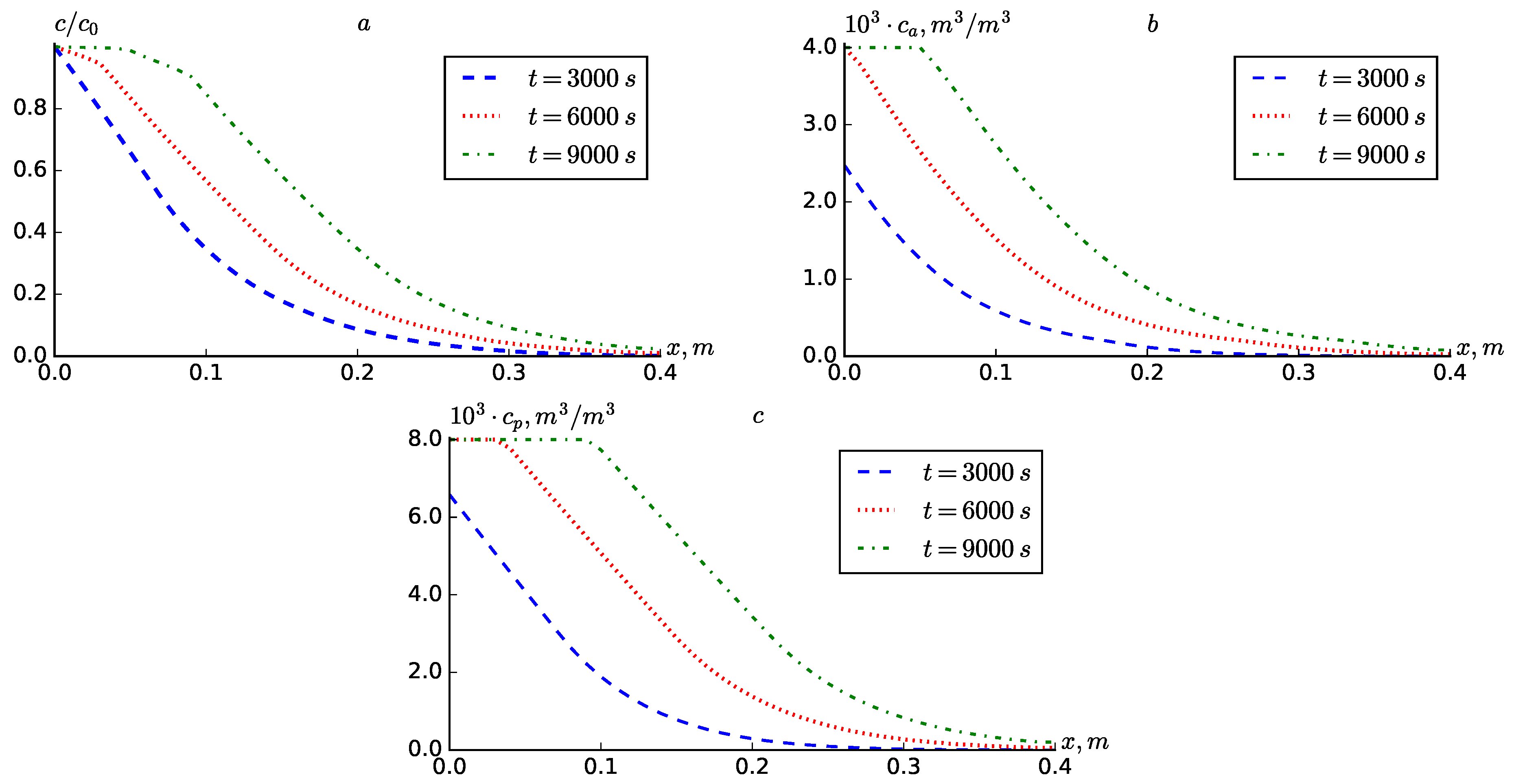
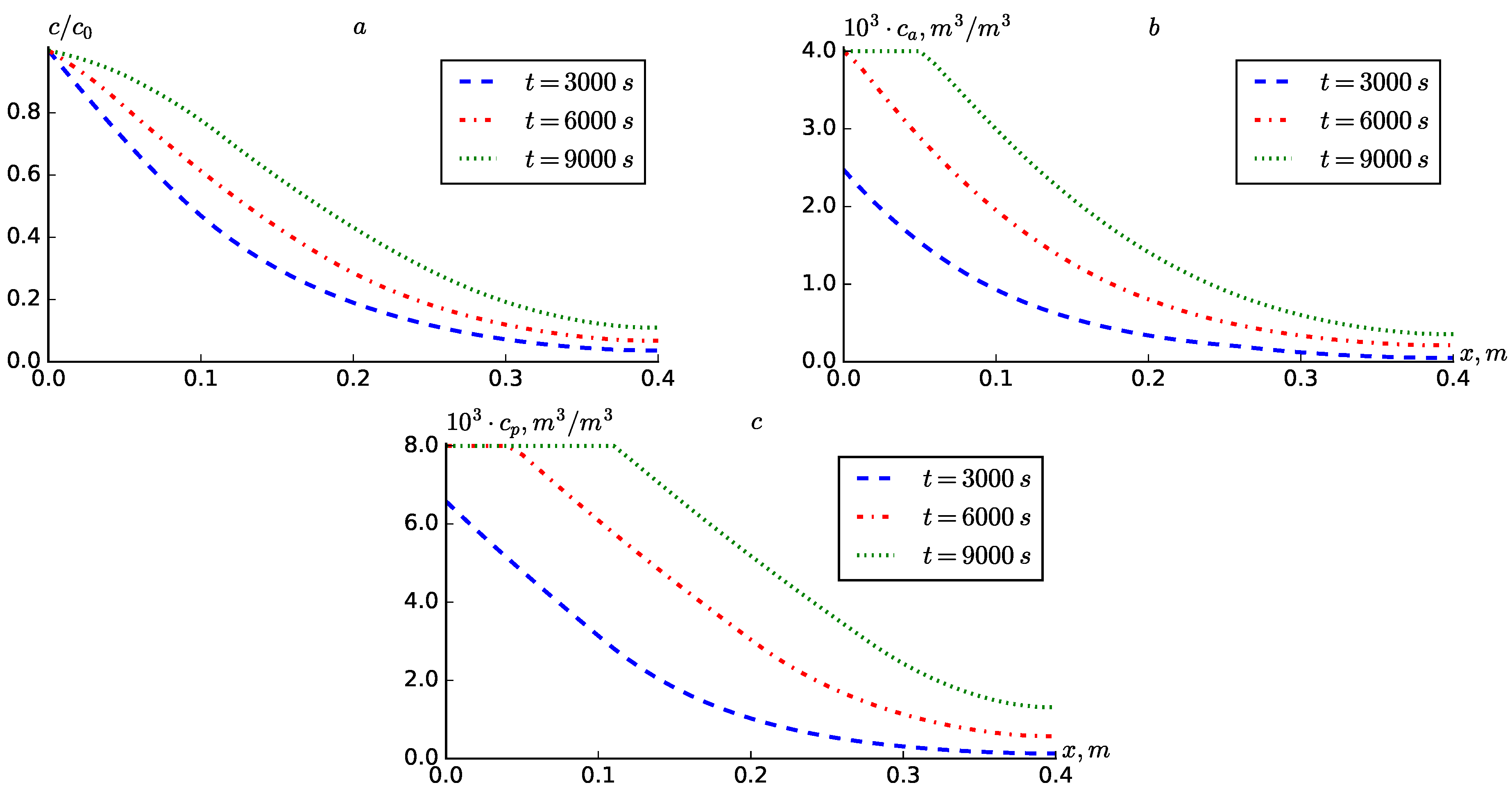
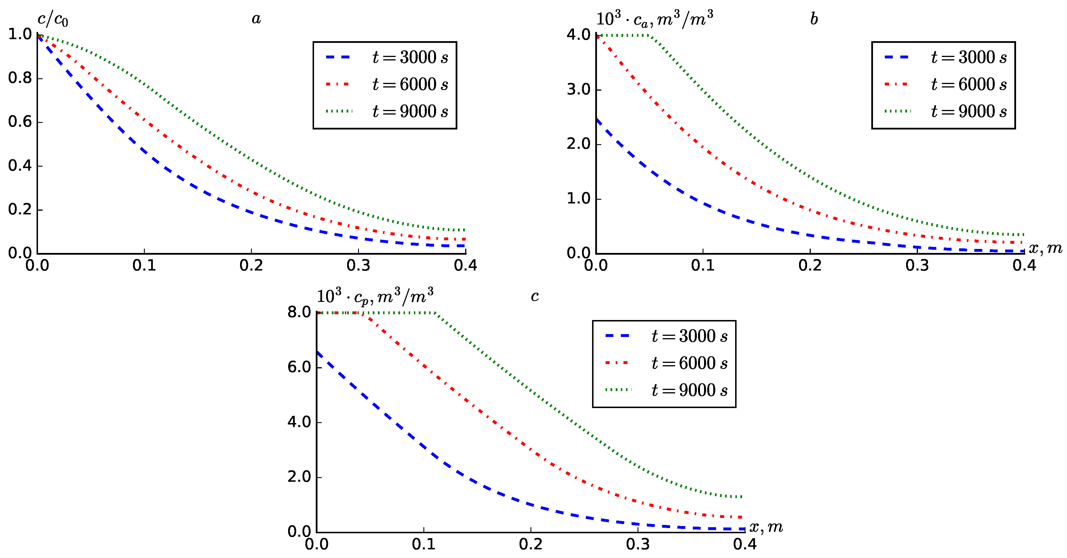
Figure 1 shows the results for the case where $D_0=0$, i.e., diffusion and hydrodynamic dispersion are not taken into account. The results are presented in the form of concentration profiles $c/c_0,c_a$ and $c_p$. Over time, the values of $c/c_0,c_a$ and $c_p$ at fixed points in the reservoir increase (Figure 1). It can be seen from the results that the solute transport process occurs more slowly when diffusion is not taken into account. Figure 1a shows that at $t=3000\mathrm{s}$, the substance concentration has only spread over a distance of $x\approx 0.32\mathrm{m}$. At this time, the adsorption in both zones has approached $x\approx 0.3\mathrm{m}$.

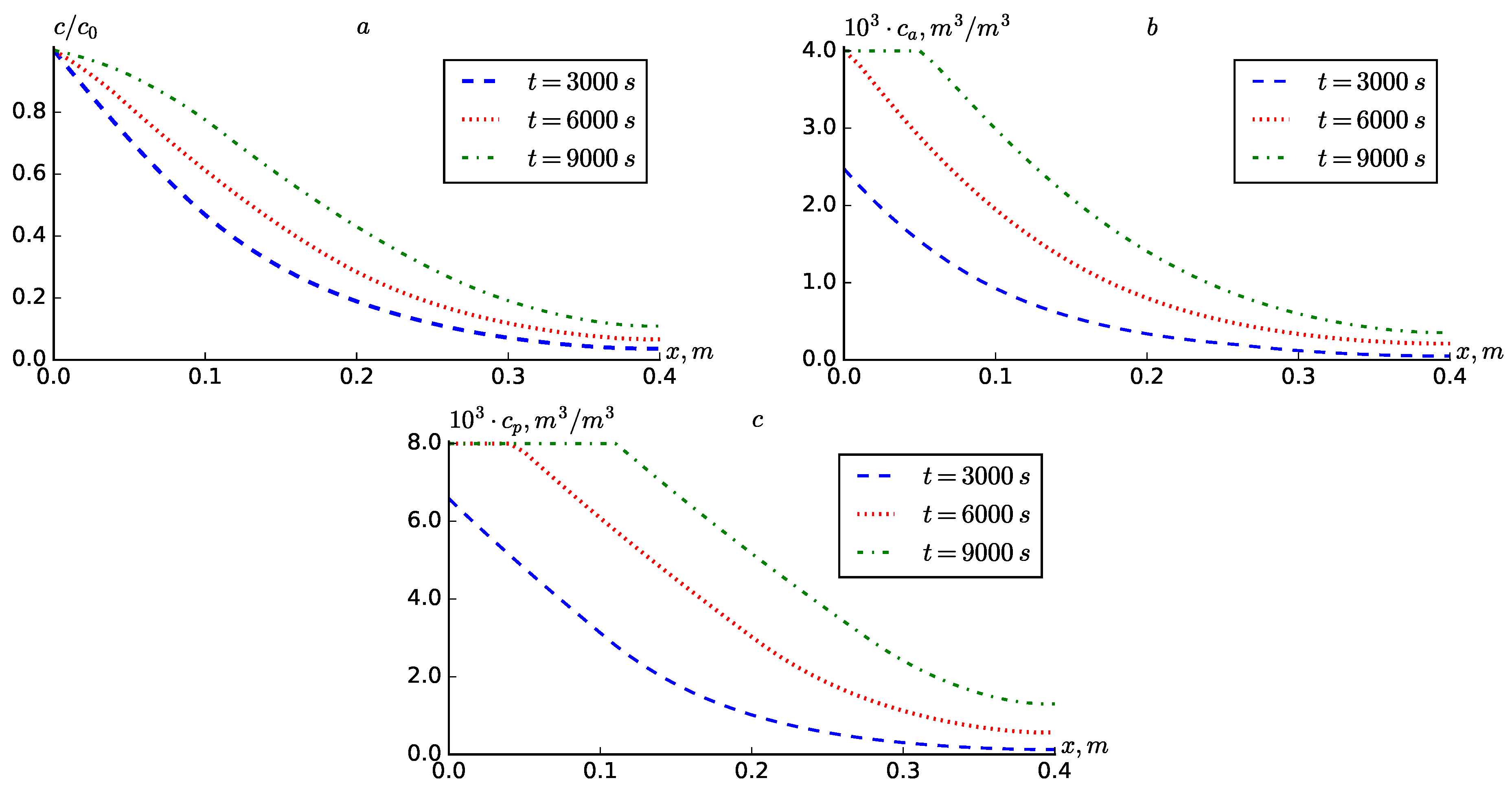
Figure 2 shows the case where $D_0=5 \times {10}^{-6}$ is in constant diffusion. Compared with Figure 1, it can be concluded that taking into account diffusion significantly accelerates the solute transport and adsorption. In particular, at $t=3000\mathrm{s}$ in Figure 2a, it can be observed that the substance concentration reaches the end of the medium ($L=0.4\mathrm{m}$). This, in turn, is observed with an increase in the concentration of the adsorbed substance in both zones (Figure 2b,c).

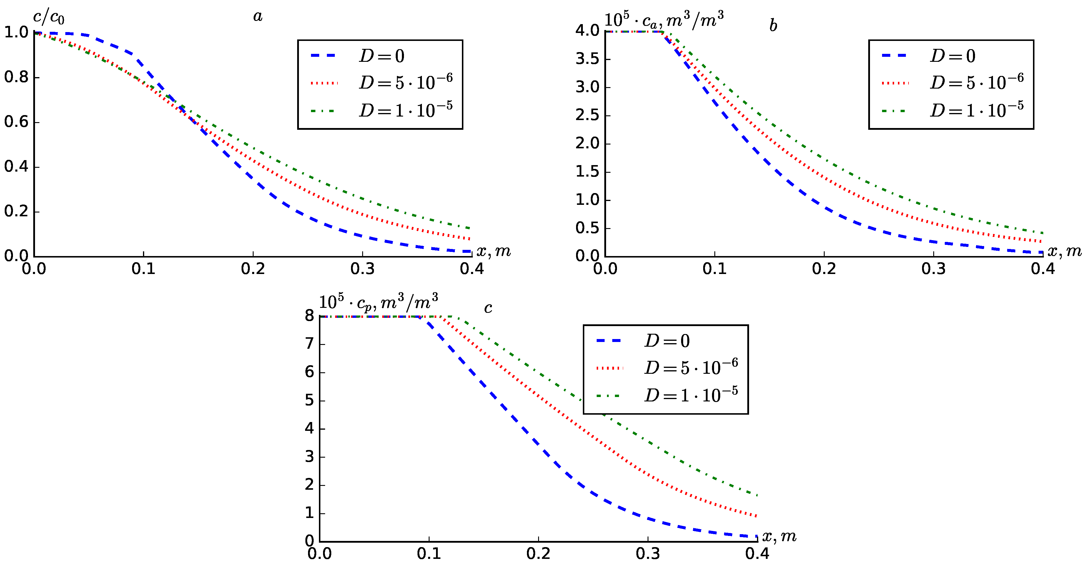
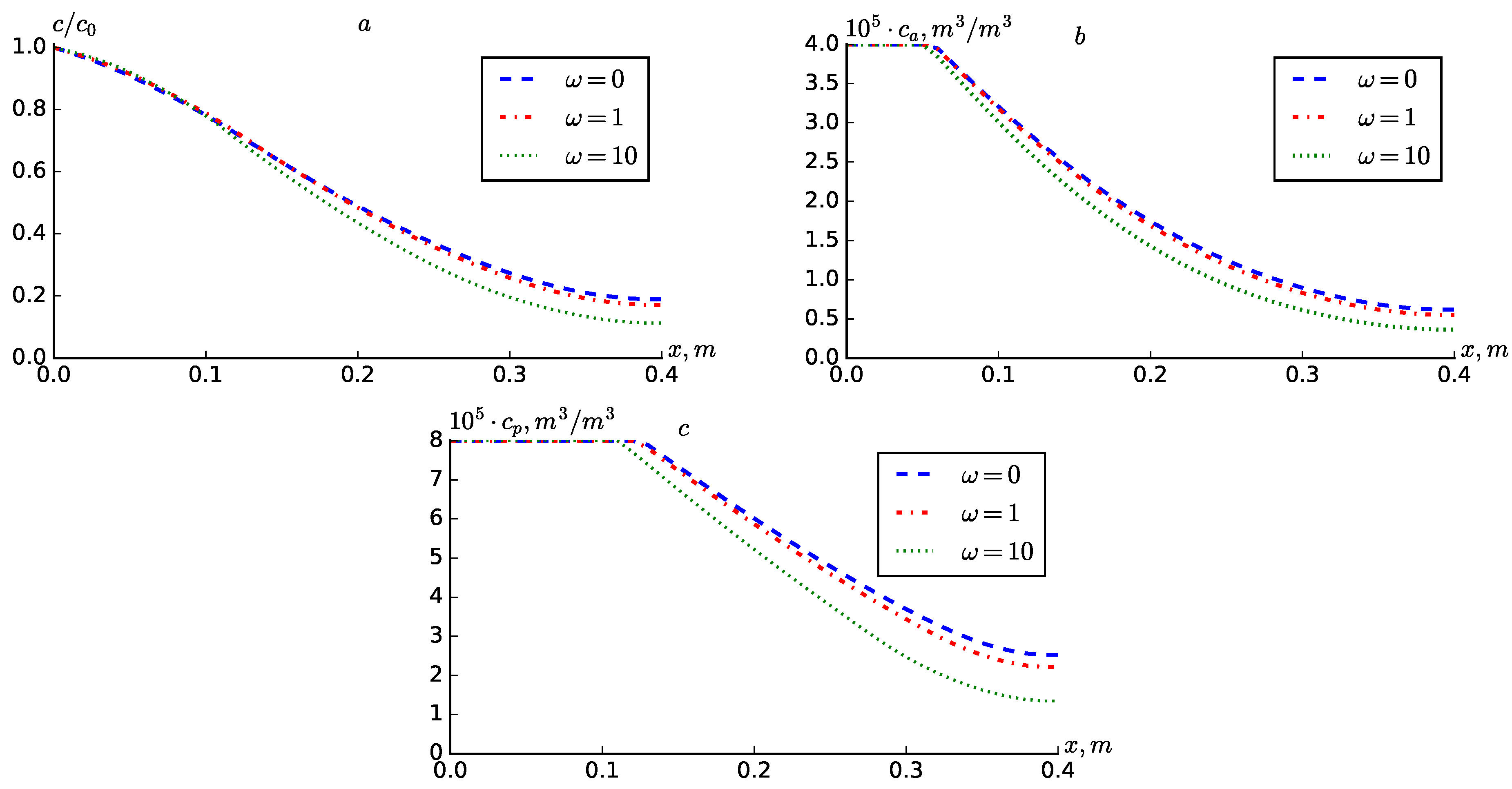
Figure 3 presents comparative graphs for different values of $D_0$. It can be seen from the graphs that an increase in the value of diffusion leads to a wider spread of the concentration profiles towards the interior of the medium. Since the scattering is less at $D_0=0$, the concentration $c/c_0$ at points closer to the point $x=0$ is greater than at the point $D_0\ne 0$, and vice versa at points further from the point $x=0$. This was not observed for the concentrations $c_a$ and $c_p$, i.e., their values increased significantly at all points of the medium with increasing diffusion.

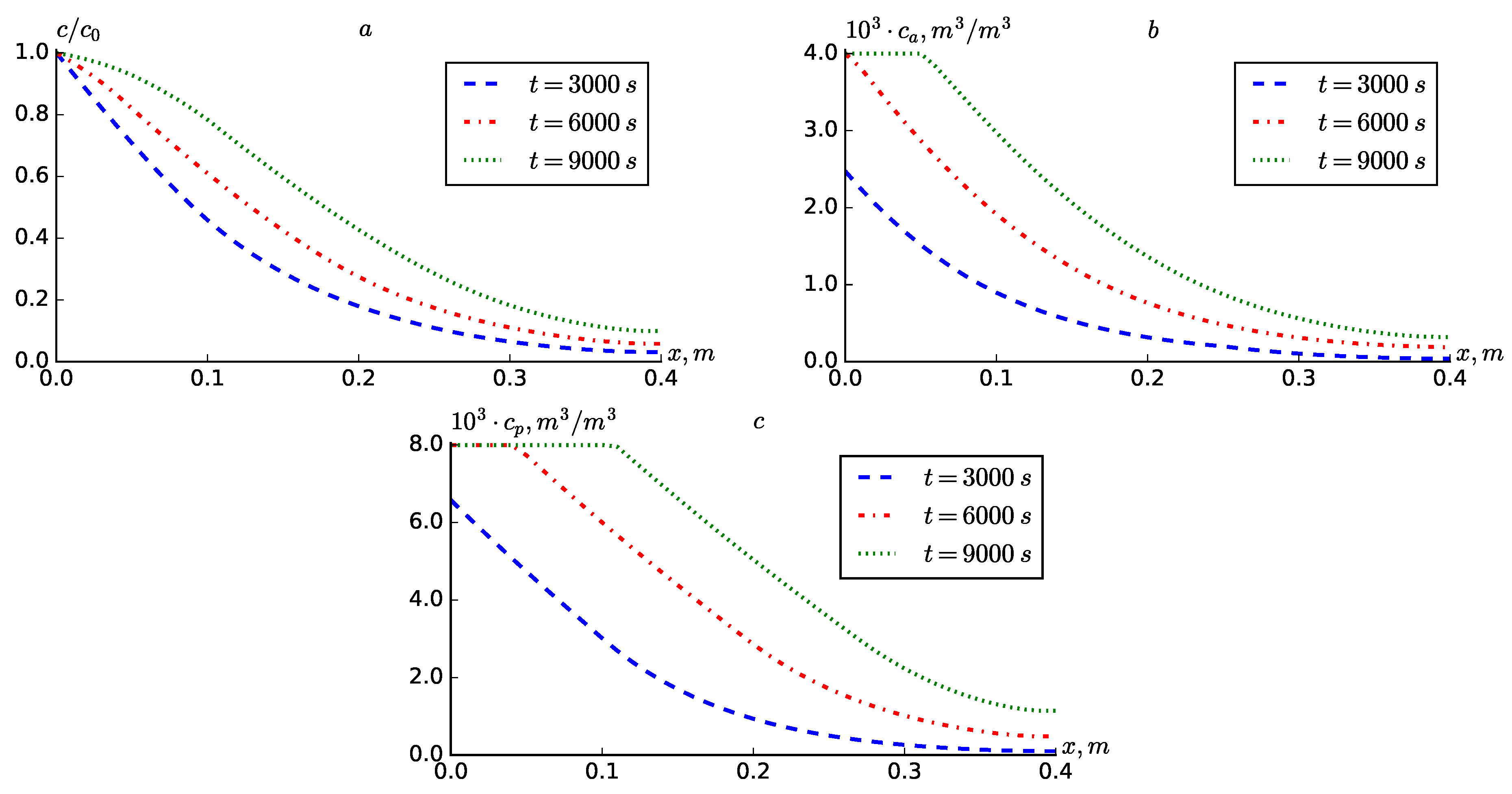
Figure 4 presents the results of numerical experiments conducted according to Formula (20), where an exponential expression depending on the coordinate for the dispersion coefficient is obtained. The results show that using Formula (20) instead of the expression $D=D_0$ increases the concentration distribution, albeit partially. This, in turn, increases the amount of adsorbed substance in both the active and passive zones.

In Figure 5, shown the solute transport and adsorption changes for different values of $\omega$ ($\omega =0,\omega =1,\omega =10$). It can be seen from the graphs that the cases with $\omega =0$ and $\omega =1$ do not differ much from each other. When $\omega =0$, it can be observed that all three concentrations increase by a very small amount compared to when $\omega =1$. However, when $\omega =10$, it can be observed that the concentrations decrease sharply at points further from the point $x=0$.

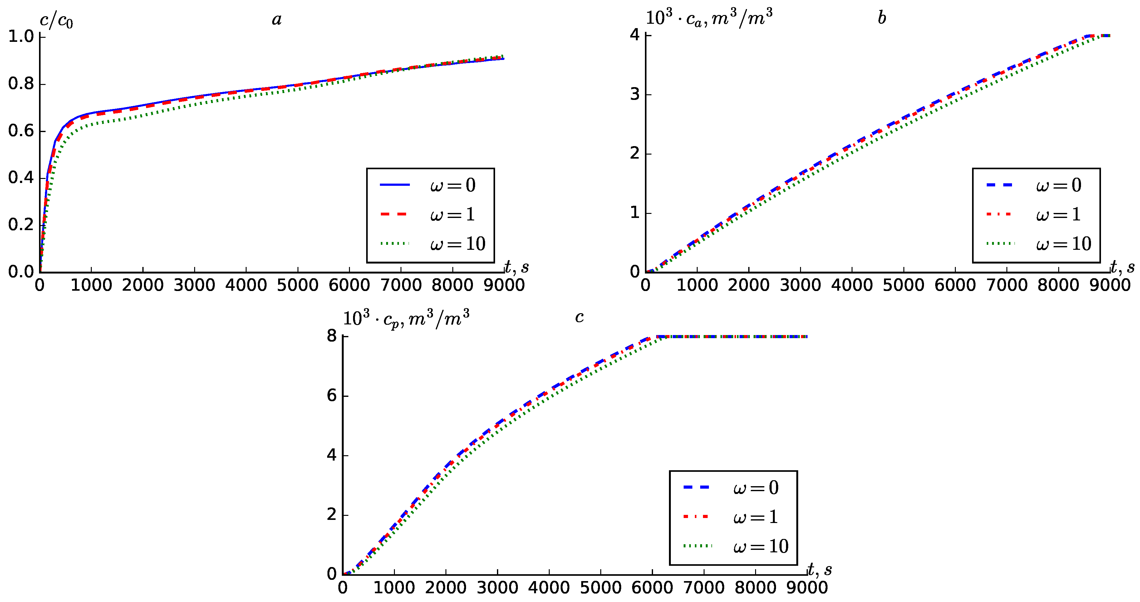
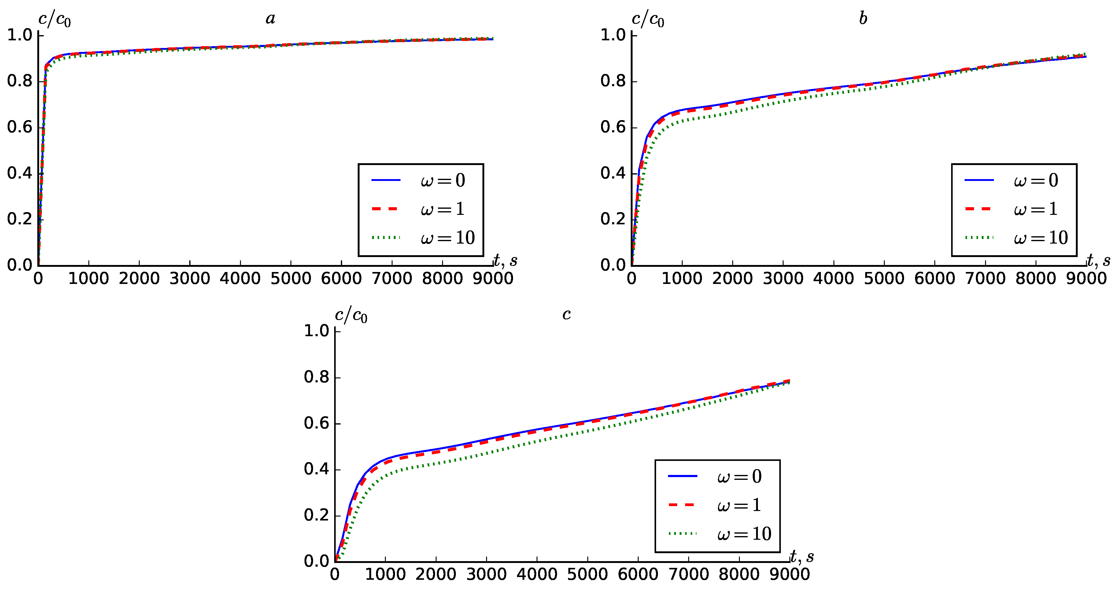
Figure 6 presents the dynamics of $c/c_0$, $c_a$ and $c_p$ at the fixed points $x=0.05$ m, for different values of $\omega$. From the graphs, it can be seen that as in Figure 5, all three concentrations increase by a very small amount with decreasing $\omega$. In particular, the results for $\omega =0$ and $\omega =1$ are very close. In order to understand the role of x in the process, we analyze the dynamics of $c/c_0$ at different fixed points and different values of $\omega$ (Figure 7). It can be concluded from the graphs that, at the point $x=0.01$, the results are very close to each other, but as the value of x increases, the difference between results also increases. This can be explained by the fact that the value of hydrodynamic dispersion depends on the value of x.

Figure 8 illustrates the outcomes of numerical experiments performed in accordance with Formula (21), resulting in a linearly increasing expression dependent on the coordinate for the dispersion coefficient. The results indicate that employing Formula (21) in place of the expression $D=D_0$ leads to a minimal increase in the concentration distribution, which may not be immediately apparent upon initial observation.

Figure 9 presents the results of numerical experiments conducted in alignment with Formula (22), yielding a parabolic decreasing function related to the coordinate for the dispersion coefficient. The findings demonstrate that utilizing Formula (22) instead of the expression $D=D_0$ yields results that are highly comparable.

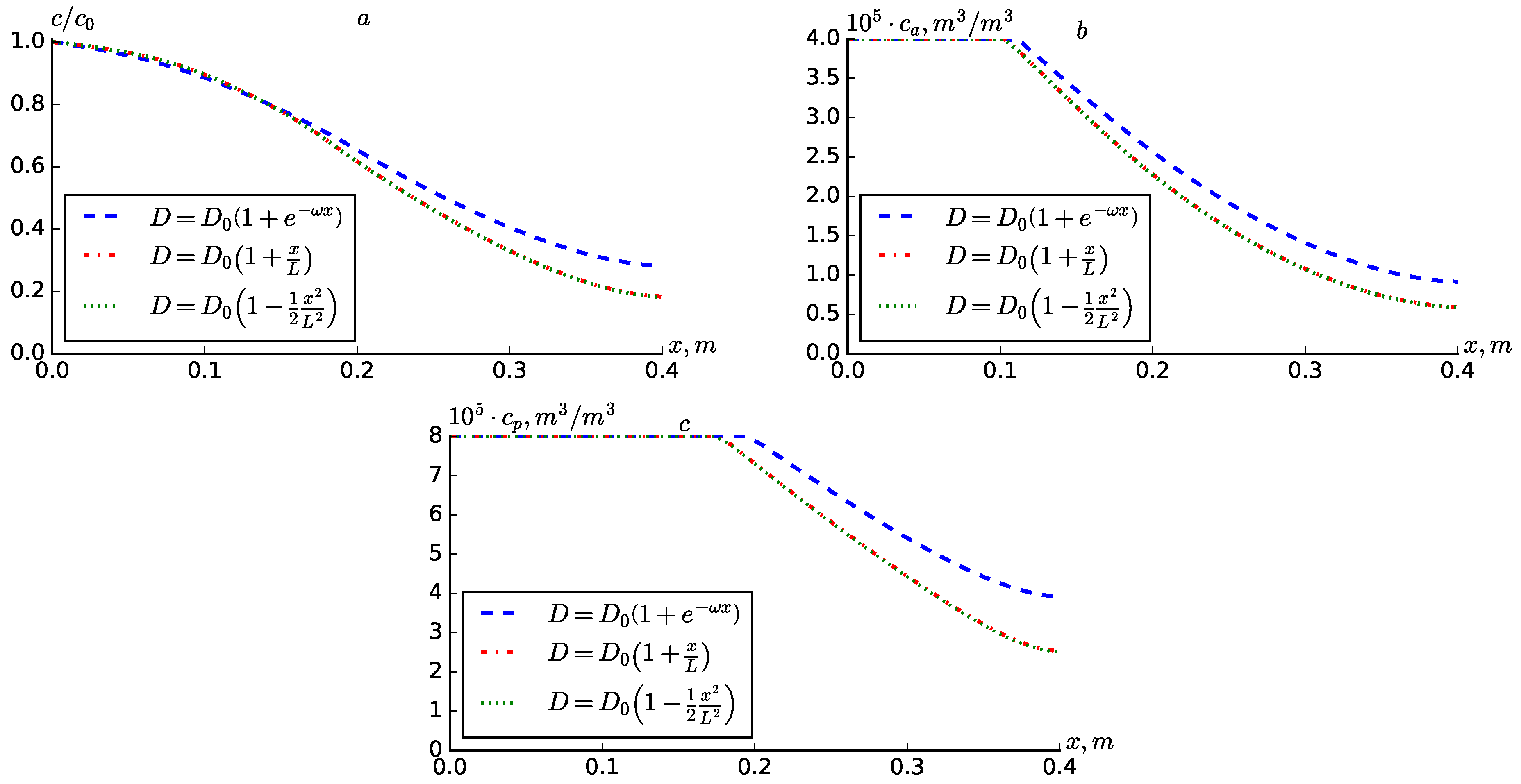
Figure 10 compares the results obtained for expressions (20) and (21) at $t=9000\mathrm{s}$. It can be seen from the results that the results obtained for expressions (21) and (22) do not differ much. In the results obtained for expression (20), the values of $c_a$ and $c_p$ are significantly larger. The values of $c/c_0$ are smaller at points closer to the point $x=0$ for expression (20) than for (21) and (22), and vice versa, the distance at $x=0$ is larger.

A comparison of

Table 1. Comparison of results of spreading concentration $c/c_0$ in fixed points for different expression of dispersion at $t=3000\mathrm{s}$.

Variation in Dispersion	Fixed Points
	$x=0$	$x=0.1$	$x=0.2$	$x=0.3$	$x=0.4$
$D=D_0$	1.0000	0.4684	0.1890	0.0715	0.0363
$\begin{array}{cc}D=D_0\left(1+e^{-\omega x}\right),\hfill & \\ \omega =1\hfill & \end{array}$	1.0000	0.5214	0.2400	0.1092	0.0666
$\begin{array}{c}D=D_0\left(1+e^{-\omega x}\right),\hfill \\ \omega =0\hfill \end{array}$	1.0000	0.5329	0.2533	0.1210	0.0779
$\begin{array}{c}D=D_0\left(1+e^{-\omega x}\right),\hfill \\ \omega =10\hfill \end{array}$	1.0000	0.4721	0.1921	0.0735	0.0377
$D=D_0\left(1+{\displaystyle \frac{x}{L}}\right)$	1.0000	0.4695	0.1900	0.0721	0.0368
$D=D_0\left(1-{\displaystyle \frac{1}{2}}{\displaystyle \frac{x^2}{L^2}}\right)$	1.0000	0.4683	0.1890	0.0715	0.0363

,

Table 2. Comparison of results of spreading concentration $c/c_0$ in fixed points for different expression of dispersion at $t=6000\mathrm{s}$.

Variation in Dispersion	Fixed Points
	$x=0$	$x=0.1$	$x=0.2$	$x=0.3$	$x=0.4$
$D=D_0$	1.0000	0.6122	0.2841	0.1186	0.0670
$\begin{array}{c}D=D_0\left(1+e^{-\omega x}\right),\hfill \\ \omega =1\hfill \end{array}$	1.0000	0.6478	0.3453	0.1670	0.1098
$\begin{array}{c}D=D_0\left(1+e^{-\omega x}\right),\hfill \\ \omega =0\hfill \end{array}$	1.0000	0.6516	0.3575	0.1804	0.1240
$\begin{array}{c}D=D_0\left(1+e^{-\omega x}\right),\hfill \\ \omega =10\hfill \end{array}$	1.0000	0.6158	0.2886	0.1215	0.0693
$D=D_0\left(1+{\displaystyle \frac{x}{L}}\right)$	1.0000	0.6131	0.2853	0.1195	0.0678
$D=D_0\left(1-{\displaystyle \frac{1}{2}}{\displaystyle \frac{x^2}{L^2}}\right)$	1.0000	0.6122	0.2840	0.1186	0.0670

and

Table 3. Comparison of results of spreading concentration $c/c_0$ in fixed points for different expression of dispersion at $t=9000\mathrm{s}$.

Variation in Dispersion	Fixed Points
	$x=0$	$x=0.1$	$x=0.2$	$x=0.3$	$x=0.4$
$D=D_0$	1.0000	0.7751	0.4303	0.1914	0.1093
$\begin{array}{c}D=D_0\left(1+e^{-\omega x}\right),\hfill \\ \omega =1\hfill \end{array}$	1.0000	0.7881	0.4841	0.2583	0.1710
$\begin{array}{c}D=D_0\left(1+e^{-\omega x}\right),\hfill \\ \omega =0\hfill \end{array}$	1.0000	0.7822	0.4898	0.2738	0.1897
$\begin{array}{c}D=D_0\left(1+e^{-\omega x}\right),\hfill \\ \omega =10\hfill \end{array}$	1.0000	0.7795	0.4357	0.1960	0.1127
$D=D_0\left(1+{\displaystyle \frac{x}{L}}\right)$	1.0000	0.7759	0.4315	0.1926	0.1104
$D=D_0\left(1-{\displaystyle \frac{1}{2}}{\displaystyle \frac{x^2}{L^2}}\right)$	1.0000	0.7751	0.4303	0.1913	0.1093

is presented for a more in-depth analysis of the results obtained using the different expressions proposed for dispersion. It can be seen from Table 1 that when the expression (20) is used, the concentrations at all fixed points are larger in the cases of $\omega =0$ and $\omega =1$ than when $D=D_0$ is constant. When $\omega =10$, the difference is not so great. When the expression (21) is used, there is a difference, although it is small compared to $D=D_0$, but for the expression (22) the difference is almost imperceptible in the results obtained with 4 digits of accuracy. This can be explained by the fact that due to the small values of x, its square becomes even smaller.

Table 2 and Table 3 present the results for larger values of time, and the conclusions made for Table 1 are once again confirmed here.

The results in Table 1, Table 2 and Table 3 indicate that introducing variable dispersion alters both the amplitude and spatial extent of solute concentration compared with the constant-dispersion case. The exponential form of dispersion produces a broader concentration front and enhanced adsorption in both active and passive regions, reflecting the higher mixing intensity near the inlet. In contrast, the linear and parabolic forms yield comparatively uniform spreading, consistent with weaker gradients of $D\left(x\right)$. These differences illustrate the sensitivity of solute transport to the spatial variation in dispersion and confirm the physical mechanisms underlying heterogeneous mixing in porous media.

5. Conclusions

This study formulated and examined a degradable-solute transport model inside a two-zone porous medium that explicitly integrates advection, spatially dependent hydrodynamic dispersion, multistage adsorption in active and passive zones, and first-order decay. A finite-difference solution method utilizing a tridiagonal solver was employed to address coordinate-dependent diffusion terms and piecewise adsorption kinetics. Numerical tests were conducted for constant dispersion and three representative spatially variable forms—exponential, linear, and parabolic—using identical hydraulic and kinetic parameters.

The simulations indicate that disregarding diffusion and dispersion significantly hinders plume progression and leads to an underestimation of both aqueous concentrations and sorbed inventory. The introduction of even minimal dispersion enhances transport throughout the domain and amplifies adsorption in both areas, resulting in reduced aqueous peaks at the input and elevated concentrations further downstream. Among the variable dispersion forms, the exponential law dispersion exhibited the most significant deviations from the constant dispersion scenario. Conversely, the linear and parabolic dispersion forms produced minimal variations at the examined length and velocity scales, indicating their relatively modest variation within specified boundaries. The sensitivity to the exponential-form parameter $\omega$ indicated that a quick decay of the elevated inlet dispersion ($\omega =10$) inhibits far-field accumulation while just slightly influencing the near-inlet profile. These results collectively indicate that the shape and scale of the dispersion function govern both the timing of breakthrough and the distribution between dissolved and sorbed masses.

The findings suggest that utilizing scale-dependent or coordinate-dependent dispersion models can significantly impact forecasts of pollutant arrival timings and retention in remedial or agricultural contexts. Augmented dispersion near sources typically results in a more extensive distribution of solute, hence enhancing sorptive absorption and potentially reducing local peak water concentrations; nevertheless, it may also expedite downstream exposure if the greater dispersion endures across significant distances. Consequently, depending on a fixed dispersion coefficient may inaccurately represent danger and cleanup timelines in systems where dispersion fluctuates with distance or hydraulic conditions.

This study is confined to one-dimensional, steady-flow scenarios with uniform porosity and simplified boundary conditions, excluding calibration to laboratory or field data. Future endeavors should broaden the framework to encompass two and three dimensions with heterogeneous characteristics, integrate it with variable-density or transient flows, investigate alternative (nonlinear) adsorption/desorption and biodegradation kinetics, and conduct systematic sensitivity and uncertainty evaluations. Integrating data-driven calibration or inverse modeling with tracer experiments would enhance the quantification of the suitable form and parameters of $D\left(x\right)$ for site-specific forecasts. Notwithstanding these constraints, this study unequivocally demonstrates that the careful selection of dispersion models is crucial for accurate predictions of degradable-solute behavior and movement in porous surfaces.