Abstract
This manuscript examines the rotational dynamics of rigid bodies in five-dimensional Euclidean space. This results in ten coupled nonlinear differential equations for angular velocities. Restricting rotations along certain axes reduces the 5D equations to sets of 4D Euler equations, which collapse to the classical 3D Euler equations. This demonstrates consistency with established mechanics. For bodies with equal principal moments of inertia (e.g., hyperspheres and Platonic solids), the rotation velocities remain constant over time. In cases with six equal and four distinct inertia moments, the solutions exhibit harmonic oscillations with frequencies determined by the initial conditions. Rotations are stable when the body spins around an axis with the largest or smallest principal moment of inertia, thus extending classical stability criteria into higher dimensions. This study defines a 5D angular momentum operator and derives commutation relations, thereby generalizing the familiar 3D and 4D cases. Additionally, it discusses the role of Pauli matrices in 5D and the implications for spin as an intrinsic property. While mathematically consistent, the hypothesis of a fifth spatial dimension is ultimately rejected since it contradicts experimental evidence. This work is valuable mainly as a theoretical framework for understanding spin and symmetry. This paper extends Euler’s equations to five dimensions (5D), demonstrates their reduction to four dimensions (4D) and three dimensions (3D), provides closed-form and oscillatory solutions under specific inertia conditions, analyzes stability, and explores quantum mechanical implications. Ultimately, it concludes that 5D space is not physically viable.
1. Rotation of Rigid Bodies
The major motivations and methodological issues are as follows:
- a.
- The motivation behind this study: This study aims to reveal new or alternative opportunities in classical and quantum mechanics.
- b.
- The significance of the study: This study provides an alternative explanation for some physical observations that cannot be satisfactorily explained by the current paradigm.
- c.
- The aim of the study: This study aims to extend the scope of physical processes and evaluate the number of new objects in the expanded context. The study centers on developing the Euler equations and subdividing 5D space into 4D subspaces. Specifically, the study explores an alternative subordination of the 4D embedding space into four 3D subspaces.
- d.
- The research methodology: The research methodology uses a non-relativistic approach to describe multidimensional rotations of solids and point-like, infinitesimally small bodies. This methodology is based on Clifford algebras and the classical quantum approach to rigid particles in multidimensional Euclidean space.
- e.
- Specific application of the study: This work represents a continuation of the investigation into rigid-body rotations in spaces of the fourth dimension [1], extending the inquiry into the fifth dimension. The results of the mathematical investigation suggest a novel interpretation of the spin phenomenon. Spin angular momentum, also referred to as “spin,” is a fundamental property inherent to all particles, irrespective of their status as elementary or composite entities. This property is intrinsic, meaning it is not dependent on spatial coordinates, and manifests as the particle’s inherent angular momentum. The application provides a new perspective on the issue of extreme imbalance between the locally observed density and the averaged density over large distances. The results show that, if short-lived heavy fundamental particles can stably exist in neighboring 3D subspaces, they can significantly contribute to the averaged density over large distances.
- f.
- The major conclusions of the study are as follows: the 4D hypothesis allows us to consider similar physical equations in four neighboring 3D subspaces and their population with imaginable objects. Some known problems could possibly be solved in this way. We conclude that there is no need for further dimensional extension to five.
1.1. Description of the Rotations
In Newtonian mechanics, a rigid body is defined as an extended solid piece of matter, whereby the relative position of any two of its points remains constant. It is evident from an intuitive standpoint that the motion of this body can be delineated in relation to an arbitrary “space-fixed” inertial reference frame with origin . This can be achieved by first fixing an arbitrary point within the body and subsequently determining the orientation of an arbitrary body-fixed Cartesian basis system [2].
The elementary rotation of the body takes place along a specific axis. According to the established principles of rotational dynamics, the axis of rotation is determined to be normal to the plane of rotation. In any given number of spatial dimensions, rotational dynamics can be characterized by mechanical properties embodied in antisymmetric rank-2 tensors [3,4,5]. The tensor of rank zero is a real number. The tensor of rank one is a vector . It is evident that the one-dimensional rotation exists in all Euclidean spaces that are characterized by a higher than one-dimensional dimensionality.
The rotation velocity over two-dimensional Euclidean subspaces is represented by an antisymmetric tensor of rank :
The plane of rotation is characterized by the two constituent vectors, which are designated as follows: . The Latin indices are running from to . The Einstein summation convention is employed in this context, stipulating that in any expression in which two equal indices emerge, the index pair must be summed over from 1 to . These rules are as follows: 1. Repeated indices are implicitly summed over. 2. It is imperative to note that each index is permitted to appear no more than twice in any given term. 3. It is imperative that each term contains identical non-repeated indices. The elementary rotation is thus characterized by the indices of both vectors and . The angular velocity (1) does not change if chooses a different origin for . The orientation of the body-fixed system relative to the is determined by the certain number of degrees of freedom, which depends upon the dimension of the space. The non-zero elements of matrix (1) can be described as generalized coordinates. Two-dimensional rotation (1) exists in all Euclidean spaces with dimensions greater than two.
The rotation velocity with respect three-dimensional Euclidean subspaces is represented by a tensor of rank :
In the 5D space, the totally antisymmetric Levi-Civita pseudo-tensor is of rank 5 (Hollmeier, 2024 [5]). For the sake of convenience and to facilitate summation, there is justification for the employment of both co- and contravariant indices. In the Euclidean space, the subscript and superscript indices can be freely exchanged, and their position is used solely to make summations more visible. Three-dimensional rotation (2) exists in all Euclidean spaces with dimensions higher than three.
The rotation velocity with respect to four-dimensional Euclidean subspaces is represented by a tensor of rank :
The four-dimensional rotation (3) exists in all Euclidean spaces with dimensions higher than four.
We calculate now the numbers of degrees of freedom for rotations of different ranks . The number of components of all tensors of different ranks is equal to the following:
The total number of all possible degrees of freedom for a given dimension is equal to the following:
1.2. Inertia Tensor
It is evident that each constituent of the momentum is a linear function of the angular velocity component. In the context of vector notation, the angular velocity vectors are interconnected through a linear transformation, which is symbolized by the rank-2 inertia tensor. The moment of inertia is defined as the angular acceleration produced by an applied torque. Angular acceleration is contingent upon three factors. Firstly, the geometry and mass distribution of the body must be taken into consideration. Secondly, the orientation of the rotation axis is important. The concept of moment of inertia, analogous to the role of mass in translational motion, signifies the body’s resistance to alterations in its state of motion. The common tensor of the moments of inertia relative to the rotation axis is a tensor of second rank, according to [6].
Accordingly, the tensor of the angular momentum, related to the rotational velocity, is represented by a rank-4 inertia tensor . In the rotation part we use the representation in the components of , with the inertia tensor [7]:
In multidimensional spaces, inertia tensors of the higher ranks manifest. The rotational velocity is related to the angular momentum by the certain rank-6 inertia tensor :
The rotational velocity could be related to the angular momentum by the certain rank-8 inertia tensor :
Equations (7) and (8) use the generalized Kronecker symbol in five-dimensional space [8,9]:
Expressions (6)–(8) result in a continuous mass density.
1.3. Angular Momentum
The vector of angular momentum, denoted by , is defined as the product of the tensor of the moment of inertia, relative to the rotation axis , and the vector of the angular velocity, [10]:
Two-dimensional angular momentum, denoted by , is defined as the product of the moment of inertia, relative to the rotation plane, , and the angular velocity, :
In accordance with the stipulations enumerated by the Einstein summation convention, in instances where an index variable is present in two separate terms within a singular expression yet remains unambiguously defined, it is conventionally interpreted as an implicit summation of the term in question across the entirety of possible values that the index might assume. The components of tensors and are skew-symmetric. Therefore, it can be concluded that their contraction product (6) is also skew-symmetric [11]. The angular momentum is the antisymmetric tensor of rank 2:
Three-dimensional angular momentum is defined as the product of the moment of inertia relative to the rotation subspace, , and the corresponding angular velocity, :
Finally, the four-dimensional angular momentum is defined as the product of the moment of inertia relative to the rotation subspace, , and the corresponding angular velocity, :
In the event that the body-fixed coordinate system BS is established at the center of mass, the kinetic energy of a rigid body is comprised of distinct components [12]. The mixed terms are eliminated here because we choose the center of gravity as the origin of . Consequently, the kinetic energy is dissociated into two distinct components: a translational component and a rotational component. The initial segment pertains to the kinetic energy of translation of the center of mass with a specific velocity. The second component is the kinetic energy of rotational motion with angular velocities about the subspaces that pass through the center of mass:
The kinetic energies (15) are the scalar integrals of the corresponding motions.
In the context of rotational motions, it can be posited that torque is equivalent to the change in angular momentum, over a specified interval of time for a given external torque :
The external torque, , is the antisymmetric tensor of rank 2. Correspondingly, the external torque is the antisymmetric tensor of rank 3, and so on. In the event of the applied external torque being set to zero, the components of angular momentum are shown to be the integrals of motion [13]. The coefficients of the characteristic polynomials of , are the integrals of motions in the corresponding cases.
2. Moments of Inertia of an Arbitrary Order of the Hyperspheres
The general sphere (or “hypersphere”) is a term used to describe the locus of a point at constant distance from a fixed point [14]. The subsequent deliberations will be curtailed on solid hyperspherical bodies with radial-dependent density distributions. The evaluation of the moments of inertia for hyperspheres of arbitrary dimensions is based on outcomes reported in the existing literature [15,16,17,18].
The volume and the surface of the sphere in the space of dimension were defined as follows [17]:
In order to perform the necessary calculations of mass moments of inertia for the hypersphere of the radius , it is first necessary to determine the moment of weight about the polar axis, which is normal with regard to the space of the sphere. This auxiliary value is equal to the following:
It has been demonstrated that the value of the inertia factor is equivalent to the specific value for hyperspheres in spaces of dimension . Given that the inertia factor remains constant under affine transformations, the same value of the inertia factor is obtained for ellipsoids in spaces of the same dimension. For the calculation, the following integral will be used (Equation 3.621 from [19])
The moment of weight about a diameter is equal to the following:
The auxiliary function is defined in Equation (20) with the following special function (21):
3. Euler’s Equations in 5D
3.1. Rotational Transformations in 5D
The principal task for the description of the classical and quantum rotational dynamics are Euler equations.
In order to proceed with the interpretation [20], it is necessary to derive the expression for the product of angular velocity and angular momentum on bivector basis. Let the body-fixed system be specifically the principal axis system. We use an orthonormal, time-invariant basis (also known as the Cartesian basis) in the five-dimensional Euclidean vector space. In 5D space, there are five basis vectors, which form a right-handed basis:
The Clifford algebra necessary for the derivation is or, equivalently, [20,21],
From the five basis vectors , ten independent bivectors could be generated:
The bivectors describe the rotations, which preserve the orientations of the 2D-planes . Second-order moments characterize the rotational inertia of a solid body. For the derivation of Euler equation, we introduce ten Euler angles:
Each Euler angle corresponds to a basic rotation of the body around a specific rotation plane. The body system BS axes, marked by indices and , remain in the rotation plane . The angle between the old vector and the new vector with the index is . Correspondingly, the same angle exists between the new and old second vectors with the index .
There are ten independent tri-vectors:
The tri-vectors describe the rotations, which preserve the orientations of the 3D-subspaces . The moments of third order are indicative of the rotation inertia of a solid body. As was shown above, for homogeneous hyperspheres, the moments of the second or third order vanish in spaces of even or odd dimensions.
The five four-vectors do not relate to any rotation because they apparently restrict four of the five degrees of freedom:
There are two final poly-vectors and . These could be referred to as a scalar and a five-vector with a single component. The set of all basis vectors of the Clifford algebra reads as follows:
The number of elements in list (27) for a given dimension is equal to the following:
In particular, .
From the angle variation, we immediately get the angular velocities over the 2D-planes or over 3D-subspaces:
Let the body-fixed system be specifically the principal axis system . It is evident that, since the consideration is situated within the principal axes of the body, the coefficients of the matrix of angular momentum will be proportional to the coefficients of angular velocity:
The products of basis bivectors in 5D are shown (Table 1: Products of basis vectors of Clifford algebra ). According to the system of classification proposed by [22], this algebra is the result of the combination of two distinct algebraic structures over the field of the quaternion algebra . There is a similarity with the group methods. It is well known that the groups and are isomorphic to each other: There are two further isomorphisms: , [23].

Table 1.
Products of basis vectors of Clifford algebra .
The expressions for the products of bivectors (23) follow from the central minor of matrix (Table 2). Table 2 is antisymmetric, but only the upper cells are shown for briefness. The display rule is as follows. The rows are labelled for ease of identification with the accents and the columns with the different accents . For example, . The table is antisymmetric because bivector products are antisymmetric: . The diagonal terms are rendered null due to the antisymmetric nature of the matrix. In the event that all the indices in both terms are different, it can be deduced that the corresponding product will also disappear, like .
Table 2.
Products of basis bi-vectors of Clifford algebra .
The expressions for the products of tri-vectors follow from the next diagonal minor of matrix (Table 3). Table 4 displays the products of four-vectors for the Clifford algebra .
Table 3.
Products of basis tri-vectors of Clifford algebra .
Table 4.
Products of basis four-vectors of Clifford algebra .
A Pascal’s triangle is a configuration of numbers arranged in the form of a triangular array. The numbers at the end of each row are set to 1, while the remaining numbers are calculated as the sum of the nearest two numbers in the preceding row. Pascal’s triangle constitutes an infinite triangular array of the binomial coefficients. Evidently, the number of unknowns exhibits a pattern consistent with that of the Pascal triangle. For compactness, the first right elements with one index are not displayed in Figure 1 and Figure 2.
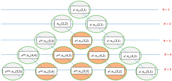
Figure 1.
The basic vectors, bi-vectors and higher products of vectors in form of the Pascal triangle. The first element are scalars (gray color), the last elements are pseudoscalars (gray color). Other elemets are multivectors (brown color).
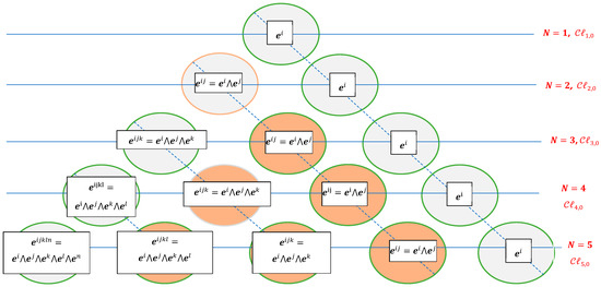
Figure 2.
The number of elements in form of the Pascal triangle. The first element are scalars (gray color), the last elements are pseudoscalars (gray color). Other elemets are multivectors (brown color).
To derive the bivector product, we use the expressions of the bivectors of an angular velocity and an angular moment with bivectors:
Analogously, the products of the tri-vectors could be formed as follows:
After the substitution of the products of six bivectors from Table 2, we can read the product of bivectors , the corresponding products of tri-vectors and four-vectors . We will study the case of the complete separation of the bi- and tri-vectors. The tri- and four-vectors appear only in the off-diagonal minors of the matrix for Clifford products.
The time derivative of the angular moment is equal to the following:
Evidently, the projections of the bivectors together with the corresponding time derivatives of the coordinates of the moments (40) deliver the components of Euler’s equations. Because the tri-vectors appear only in the off-diagonal minors of the matrix for Clifford products, the rotations , and decouple. The tri-vector rotation plays no role in the subsequent evaluations.
Only the time derivatives of the bivectors are displayed below. The derivatives that lead to the Euler equations for the poly-vectors could be developed analogously using the above method. The components of the product of the bivectors read as follows:
With the expression (38) for the moments of inertia (11), the angular momentum and its time derivative are:
The combination of Equations (38) and (40) results in the set of Euler equations for the bi-vector rotations:
The calculation of product of bivectors uses Table 2 for calculation of the products of bivectors. For the , , such that there are 10 components of Euler’s equations in five-dimensional space. The projections of the products of bivectors together with the corresponding time derivatives of the moments deliver once again the Equations (41)–(50).
The are coupled second-order differential equations for components of the tensor . The set of Euler’s equations has the disadvantage that the torque components are related to the body-fixed . The components are therefore generally time-dependent, and this time dependence depends on the body’s motion. In the following, we limit ourselves to the force-free case .
Ten Equations (41)–(50) reduce to the trio of 4D-equations, if the components of rotations in the certain 4D-projection of the 5D-space disappear.
3.2. Reduction of 5D to the 4D Rotations
3.2.1. Rotation over Axis One Restricted
If the rotation with respect to axis 1 is locked, we get:
The equations with the locked rotations are satisfied identically, and the remaining six equations condense to:
These equations describe the rotation of the rigid in four-dimensional projection of the 4D space.
3.2.2. Rotation over Axis Two Restricted
Accordingly, if the rotation with respect to the axis 2 is blocked:
The Equations (41) and (45)–(47) erased, and the remaining six equations condense to:
These equations describe the rotation of the rigid in four -dimensional projection of the 4D space.
3.2.3. Rotation over Axis Three Restricted
If rotation around axis 3 is jammed, the result is as follows:
The Equations (42), (45), (48) and (49) erased, and the remaining six equations condense to:
These equations describe the rotation of the rigid in four -dimensional projection of the 4D space.
3.2.4. Rotation over Axis Four Restricted
If the rotation with respect to the axis 4 is frozen, we have:
The Equations (44), (47), (49) and (50) erased, and the remaining six equations condense to:
These equations describe the rotation of the rigid in four -dimensional projection of the 4D space.
3.2.5. Rotation over Axis Five Restricted
Finally, if the rotation with respect to axis 5 is restricted, the following equations apply:
The Equations (44), (47), (49) and (50) erased, and the remaining six equations condense to:
These equations describe the rotation of the rigid in four -dimensional projection of the 4D space.
Finally, the sequence of equations was arranged into five sextets, with the purpose of describing the rotations in the five 4D subspaces of the 5D Euclidean space:
Evidently, that each of 4D equations reduces further if an additional degree of freedom will be fixed. We show this process on the following examples.
Restriction of an Additional Rotation
If the rotation with respect to the axis 4 is additionally fixed, we get the restricted three rotations from six possible in 4D:
The equations, which involved the rotation about the axis 4 will be satisfied identically. The remaining three equations over the axes condense to the classical Euler equations in 3D [6]:
The analogous technique could be applied to the further restriction of rotation about other axes. The trios of Euler equations are derived from the six aforementioned equations, Equation (88) to (90), through cyclical index substitutions.
Consequently, the ten equations in 5D project into five sextets of equations in the 4D spaces (52) to (85). Each sextet of equations in the certain 4D space then dissolves into four triads of the corresponding classical Euler equations in four enclosed 3D spaces.
4. Solutions of the Euler Equations in 5D Spaces
4.1. All Moments of Inertia Equal
The system of nonlinear ordinary differential Equations (41)–(50) is nonlinear and depend upon ten initial conditions and ten fixed components of inertia tensor. In some special cases the system (41)–(50) allows the closed form solutions. In the initial phase of this investigation, we shall establish the solution to the Euler equations in the case of an equal moment of inertia across all possible axes of rotation:
The Platonic bodies and hyperspheres satisfy this condition. For such bodies all gyration radii are equal. In this case the second term in all left sides of the Equations (41)–(50) vanish. The time derivatives of the rotation components nullify in the absence of the external moments:
Consequently, it is evident that all components of the rotation velocity are sustained over a given period of time. It can be posited that this behavior holds in all multidimensional Euclidean spaces.
4.2. The Equal Moments with One Quartet of Different Moments of Inertia
The second case corresponds to six equal principal moments of inertia with four distinct principal moment. In the absence of any restrictions, the equal principal moments of inertia are set to two, and the distinct moments are referred to as :
The aforementioned Equations (41)–(50) can be simplified to six nullifying expressions and four linear ordinary differential equations with constant coefficients:
The resolution (95)–(97), (99), (100) and (102) of six ordinary differential equations of a nullifying nature guarantees that the six rotation velocities remain constant. It is evident that the coefficients of four additional ordinary differential equations are contingent upon the initial six constant velocities :
The Equations (105)–(108) are the linear ordinary differential equations of the first order with the constant coefficients. The closed-form solutions of Equations (105)–(108) will be sought using the exponential ansatz ():
With the ansatz (110) the ordinary differential equations reduce to the system of linear algebraic equations with the eigenvalue parameter
The eigenvalue problem (111)–(114) can be written in matrix form:
It is notable that the matrix must be antisymmetric, as can be seen from the above equation.
It is well known that some boundary value problems have unique solutions, while others only have solutions if certain solvability conditions are met [24]. The nontrivial solvability condition of the eigenvalue problem follows from the Fredholm Alternative Theorem [25]. In the above case, the determinant of the matrix must vanish for a nontrivial solution to exist:
From Equations (116)–(118) follows, that the fundamental frequency of the oscillation solution (110) is the function of the initial six constant velocities:
The rotation velocities are harmonically oscillating functions. The oscillation periods of the third last velocities depend on the six constant velocities.
Evidently, that the equivalent results could be obtained in four other cases:
The constant velocities will be correspondingly equal to:
The oscillating frequencies of the rest degree of freedom will be given from the solution of Equation (116):
5. Stability of the Rotations
Consider a body rotating about the one principal axis with the certain angular velocity . Assume a small impulsive moment that initiates a small rotation about the other axes and thereafter the motion proceeds with no applied external moments. For this case, Euler’s equations become (41)–(50) with the zero right terms. We examine the question of stability to small perturbations, rotations about the other axes of magnitude of a small parameter .
For example, we study the stability of the rotation . In the first example, we assume the solution in the following form:
After substitution of the Equations (130) and (131) in the Equations (41)–(50), we can find, that the four equations will be satisfied in linear terms of . The remaining six equations reduce to:
We used the following notations for the briefness:
The Equations (132) and (139)–(141) leads in the first approximation with respect to to the constant angular velocities:
The remaining equations could be grouped into pairs. One group consists of Equations (133) and (136). The solution to the first group of equations is as follows:
The second group consists of Equations (134) and (137). The second group of equations has a solution:
The third group comprises a series of Equations (135) and (138). Their solution reads as:
Assume at first, that the principal rotation axis rotation circular frequency the axis with the highest principal moment of inertia:
It is evident that, in the event of the inequalities being satisfied, all three frequencies of the oscillations will be positive real values. It can thus be concluded that if rotation occurs over the axis with the highest principal moment of inertia, then the rotation is stable with oscillations of three groups of order epsilon.
It should be posited for a second that the principal rotation axis is circular in its frequency of rotation (Ω), and that it is the axis that possesses the lowest principal moment inertia.
In the event of the inequalities being satisfied, it can be demonstrated that all three frequencies of the oscillations will be positive real values once again. It can thus be concluded that if rotation occurs over the axis with the lowest principal moment of inertia, then the rotation is stable with oscillations of three groups of order as well.
6. Quantum Angular Momentum in 5D Space
For the derivation of the expressions of the angular momentum in spaces fifth dimension we apply the common principles of quantum mechanics [26]. It is evident that conducting a direct physical experiment to validate the above equations is actually not a viable option. At the fundamental level, there are discernible physical observations that lend credence to the hypothesis. It is hypothesized that infinitesimally small rotations in five-dimensional space, characterized by Cartesian coordinates , and , occur. The particles involved in such a rotation are characterized by the following parameters (24). The following expression may be regarded as the angular momentum operator:
The components of the angular momentum operator (155) are the follows:
Consider now two arbitrary differential operators in matrix form:
The components of both differential operators are the linear partial differential operators of the first order with respect to spatial variables .
The products of two arbitrary differential operators and from (157) could be calculated using the already known formula (38):
Evidently, that the products in (158) symbolize the linear partial differential operators of the order two with respect to spatial variables .
From Equation (158) we get the commutation relations for the operators. Remarkably, that if ,
The Equation (159) is valid in 5D Euclidean space. In this particular instance, the product of two operators results in the shortening of the second-order powers.
It is evident that analogous formulae can be observed in lower-dimensional spaces. The corresponding expression 4D space reads: . In three-dimensional space, the conventional formula is employed: .
In order to derive the law of conservation of momentum, it was necessary to make use of the homogeneity of space relative to a closed system of particles. In addition to its homogeneity, space exhibits the property of isotropy. In accordance with the aforementioned principle, all directions within the system are considered to be equivalent. It is an irrefutable fact that a closed system is incapable of undergoing change when the system as a whole undergoes rotation. The angle is arbitrary, as is the axis. It is imperative that this condition be fulfilled for an arbitrary infinitely small rotation.
It may be hypothesized that the rotation of different types facilitates the transfer of quantum energy units between them.
6.1. Pauli Matrices in 5D Space
Consider a composite particle, such as a solid rotator, which translates as a whole and has a specific internal state. In addition to having an internal energy, it also has an angular momentum of a specific magnitude due to the motion of its constituent particles. Translational energy is irrelevant to our study. The center of mass of the 5D composite particle can be considered at rest. For a given angular momentum value, there are different possible orientations in space. A key feature of angular momentum in quantum mechanics is that it determines the symmetry properties of a system’s states with respect to rotations in space. When the coordinates are rotated, the wave functions corresponding to different angular momentum values are transformed into combinations of one another. In this formulation, the origin of the angular momentum becomes irrelevant, and the concept of “intrinsic” angular momentum emerges naturally. This must be ascribed to the particle, regardless of whether it is “composite” or “elementary”.
In quantum mechanics, therefore, an elementary particle must be assigned a certain inherent angular momentum that is unconnected with its motion in space. This property of elementary particles is unique to quantum theory and therefore cannot be interpreted classically. The intrinsic angular momentum of a particle is known as its ‘spin’, as opposed to the angular momentum resulting from its motion in space, known as ‘orbital angular momentum’. The particle in question may be elementary or composite, but may behave in some respects like an elementary particle (e.g., an atomic nucleus). The spin of a particle (measured in units of Planck’s constant, like orbital angular momentum) is denoted by . In this section, we will not be concerned with the dependence of the wave.
Please note that the function operates on the coordinates. For instance, when discussing the behavior of the wave function of a system under rotation, we can assume the particle is at the origin. This ensures the coordinates remain unchanged by such a rotation, and the results obtained will provide valuable insights into the wave function’s behavior in relation to the spin variable.
In the context of a particle with zero spin, it is important to note that the wave function for such particles is characterized by a single, unaltered component when subjected to coordinate system rotations. This component is referred to as a scalar. In order to understand the wave functions of particles with non-zero spin, it is essential to consider their behavior under rotations about a single axis.
Since the various components of angular momentum do not commute, they are incommensurable. The square of the angular momentum operator, on the other hand, commutes with all components and can therefore be measured simultaneously with any component.
The corresponding eigenstates of the angular momentum operator are called angular momentum eigenstates. They can be characterized by the eigenvalues. A state is defined by the two quantum numbers that satisfy the following two eigenvalue equations [12]. In 3D Euclidean space, Pauli matrices were originally introduced in quantum mechanics to satisfy the fundamental commutation rules of the components of the spin operator.
The real Pauli matrices in 5D correspond to the dimension of space and are antisymmetric trace-free matrices. Elementary rotation matrices represent the transformation matrices for a rotation of 90° in a fixed plane with the following indices . The subindices denote the Pauli matrix, but not its components. The Pauli matrices are derived from elementary rotational matrices through the implementation of the anti-symmetrize operation on the aforementioned rotational matrix elements:
The symbol denotes the transposition of the matrix , . The number of Pauli matrices correspond to the dimension of the angular momentum. Within the framework of 5D space, there exist ten distinct Pauli matrices of different genera:
The Euclidean norm is equal to the largest singular value of a matrix [8,27]. The Euclidean norms of all six Pauli matrices (161)–(166) are equal to one:
The sum of all Pauli matrices in 4D reads as follows:
6.2. Commutation Relations Between Pauli Matrices in 5D Space
It is imperative to articulate the commutation relations between the real Pauli matrices. The classical commutation relations in 3D space are valid only in the space with the vector product [26]. These commutation relations are used in the derivation of the Euler equations in 3D. It is evident that the commutation relations in three dimensions comprise a single term, and each of the three-dimensional Euler equations incorporates a single product term [10]. Correspondingly, the equations of the quantum rotator in three dimensions also incorporate a single product term [28,29].
In each of the 5D spaces, the commutation relations appear in three product terms:
The summation is performed over the indices 1 to 5. The terms with two equal indices vanish because of the skew-symmetry of the matrices . Consequently, in each equation remain three pairs of matrix products. The similar commutation relations with three cross-terms were used in the neighboring equations for the quantum rotator. Equation (173) can be associated with ten hypothetical quantum states in 5D.
6.3. Separation of 5D Space into Five 4D Subspaces
It is a noteworthy observation that merits further consideration. The hypothetical 5D space could be separated into four 4D subspaces (Table 5: Separation of 5D space into five 4D subspaces with the Pauli matrices of different genus). The most interesting subspace will be considered in the next section.
Table 5.
Separation of 5D space into five 4D subspaces with the Pauli matrices of different genera.
Each of 3D subspaces contains three real Pauli matrices. In 3D subspace with Latin number “I”, the index 1 of Pauli matrices is absent. In three-dimensional space, the index “II” of the Pauli matrices is also absent. It is evident that within the three-dimensional spatial domain, characterized by the Latin letter “III”, the index “3” in each Pauli matrix does not exist. In subspace “IV” there is no index “4”. It can thus be concluded that each of the three-dimensional subspaces is populated by particles that comprise precisely three Pauli matrices of six different genera. Evidently, each of the Pauli matrices of different genera appear two times in 4D. It could be an interesting remark about the population of the four 3D subspaces, as shown in Table 6, Table 7, Table 8, Table 9 and Table 10.
Table 6.
Separation of 4D space into four 3D subspaces with the Pauli matrices of different genera.
Table 7.
Separation of 4D space into four 3D subspaces with the Pauli matrices of different genera.
Table 8.
Separation of 4D space into four 3D subspaces with the Pauli matrices of different genera.
Table 9.
Separation of 4D space into four 3D subspaces with the Pauli matrices of different genera.
Table 10.
Separation of 4D space into four 3D subspaces with the Pauli matrices of different genera.
The Pascal triangle can be used to display the independent rotational degrees of freedom in different-dimensional Euclidean space (Figure 3). The mirror-symmetrical table depicts the corresponding anti-particles.
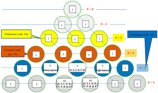
Figure 3.
Pascal triangle displaying independent rotational degrees of freedom for different dimensions of Euclidean space N. The elements for are marked with yellow color. The elements in dimension are in brown, are in blue and are in gray colors.
The hypothesis of five-dimensionality posits a conclusion regarding the fundamental particles at ten, thereby essentially foreclosing this possibility. Consequently, the hypothesis of five-dimensionality is incompatible with the factual physical experiments and must therefore be rejected. It is imaginable that the dimension of space is contingent on the scale of physical experiments, as outlined in the study on the equations of mathematical physics in spaces of variable dimensions [30].
7. Hypothetical Four-Dimensional Subspace “”
7.1. 3D Subspaces of the Hypothetical 4D Subspace “”
There are four 4D subspaces of a Euclidean 5D space, as displayed in Table 5 (Separation of 5D space into five 4D subspaces with the Pauli matrices of different genus). In the 4D subspace “” with the coordinates , the matrices with the index 5 disappear. The selection of the 4D geometry is predicated on a single, compelling argument. It is a well-established fact that the actual physical paradigm is comprised of six fundamental particles [31]. The aforementioned paradigm is indicative of the four-dimensional embedding space.
The 4D-commutation relations with two product terms appear for Pauli matrices (161)–(166) read as follows:
Of relevance to physical applications are perhaps only a small number of three-dimensional subspaces. Namely, 3D subspace IV is pertinent for observable physical applications [32]. The forementioned equations could be verified expeditiously by employing the multiplication of the Pauli matrices (161)–(166). The signs in the above equations correspond to the alternation of signs in Euler equations and in the consistent quantum equations. It has been established that Equation (174) is to be associated with six common names of the quantum states in the 4D subspace “”.
In the context of three-dimensional projections, the potential for interaction exists, analogous to the principles of classical electrodynamics in each separate of I, II, III, IV. This information is presented in Table 10. The sole discrepancy lies in the varying charge, which is associated with the specified 3D projection. The absence of electrodynamic interaction is evident when considering the disparate projections. The hypothetical 4D charges of the 3D projections of space E are illustrated in Table 11. The masses for the populations of the subspaces I, II, III, IV are shown in GeV. The hypothesis posits that each object is exclusively the projection of a single 4D object onto six 3D projections. Consequently, the number of projections in 4D space E, denoted by , is constant for each object. The light projections are precisely as frequent as the heavy projections. The heavy objects are concealed within the three-dimensional “IV” sub-space due to their association with other three-dimensional sub-spaces, designated “I”, “II” and “III”, which are not permanently observable. It is hypothesized that high-energy experimental facilities possess the capacity to manipulate the 4D object for a quantum period of time. During this interval, the 4D object maintains an erroneous spatial orientation. The misorientation of the 4D object is evidently energetically unfavorable and consequently unstable. Due to this inherent instability, the , T, and projections are only observable for a quantum period of time. The object undergoes a retrograde rotation, reorienting itself to its stable position, thereby dissipating a specific amount of energy. It is conceivable that the omission of photons occurs in disparate three-dimensional subspaces. It is hypothesized that the total mass of the 4D object contributes to a hypothetical mass-energy density in the embedding Minkowski space of E with the Clifford algebra of type :
Table 11.
Hypothetical 4D charges of the 3D projections of the space .
7.2. Evaluation of Charges
It is hypothesized that the classical scalar fields act in the subspaces “I”, “II”, “III” and “IV”. These hypothetical fields have certain charges. These fields are assumed to resemble the usual electrodynamic field. The electric and magnetic fields of the electrodynamics, i.e., the electric and magnetic field strength, are described by four potentials. The existence of specific quasi-electrical charges in the subspaces “I”, “II”, and “” is hypothesized. Each projection is characterized by four quasi-electrical charges. The charges of each projection are presented by the vectors in 4D subspaces (Table 11). The vectors are given by the four initially unknown amplitudes and an initial rotation:
The 4-vectors of the charges are given by the rotated vector :
We assume that all rotation angles are equal to one initially unknown value:
The total charge of six 3D projections of a single 4D particle is equal to the following:
We assume that the summary charges of all four components is equal to one. This behaviour is known by the summation of the charges of the common quarks in 3D space [32,33]. From this hypothesis, we get from (183) four equations:
The resolution of four linear algebraic Equation (184) gives the following values of the amplitudes:
Formulas (185)–(187) deliver the solution for the charges with one arbitrary constant . We can determine this constant from the condition that the common electrical charge of the particle is equal to zero. This condition expresses the known neutral electrical charge of the neutron. This leads us to the algebraic equation that the fourth component of the vector must vanish:
The nominator of Equation (188) is the nonlinear algebraic equation with respect to . Its solution is given by the following formula:
Of the five roots of the second equation in (189), there are four complex and one real root. A real root of Equation (189) is , which leads to the following:
The substitution of (185)–(187) and (190) into the expressions for 4-vectors gives the following values of 4-charges:
The charge of the particle must correspond to the positive unit charge of proton. From Equation (191) we get the value All values in Equation (191) must be multiplied by the correction factor The corrected values result in the 4-vectors:
After the evaluation of the charges, we substitute the vectors (192) into Table 11. With the calculated values for charges, it is possible to calculate the summary charges of three-folded particles (Table 12, Table 13, Table 14 and Table 15).
Table 12.
Combinations of 3D projections in the three-folded fermions.
Table 13.
Combinations of 3D projections in the three-folded fermions.
Table 14.
Combinations of 3D projections in the three-folded fermions.
Table 15.
Combinations of 3D projections in the three-folded fermions.
Table 12 presents a comprehensive overview of the combinations of 3D projections in the triple fermions. As demonstrated in Table 13, the configurations of 3D projections manifest in three-folded fermions. Table 14 displays combinations of 3D projections of in three-dimensional fermions (3D Projections ). As shown in Table 15, the combinations of 3D projections in the fermions, composed of three corresponding projections, are presented. All these values are purely hypothetical and preliminary. More profound models are expected to be developed in future studies.
A note on the population of the second and fourth cells in row of the Pascal triangle (Figure 3): The cells correspond to four basis poly-vectors and basis vectors , as shown in Figure 1. We expect these places to be populated by heavy and light leptons. In the “Standard Model,” the heavy leptons are the electron, the tau, and the muon [31,33]. The light leptons are the electron neutrino, the tau neutrino, and the muon neutrino. Consequently, both groups of light and heavy leptons contain three particles. The proposed classification, based on Clifford algebras in four-dimensional space, predicts four leptons in each cell. In each group, the presence of one lepton is conspicuously absent. The eventual discovery of the missing leptons in each group would support the four-dimensional hypothesis.
7.3. Alternative Evaluation of Charges
Another hypothesis is put forward that alternative quasi-electrical charges exist in the subspaces designated “I”, “II”, and “”. Each projection is characterized by four quasi-electrical charges (Table 16). The charges of each projection are presented by the alternative vectors in 4D spaces.
Table 16.
Alternative setting of 4D charges of the 3D projections of the space .
It would be worthwhile to calculate the masses of the projections, which are oriented in different subspaces (Table 17). The summary masses of all projections oriented to different subspaces differ significantly. The ground is the substantial mass of the T projection, which surpasses all other projections. It is possible that the presented arguments will provide an alternative viewpoint on the appearance of weak isospin and color charge.
Table 17.
Mass and percentage share of the mass of different subspaces.
8. Conclusions
The manuscript embarks on an investigation into the rotational behavior of rigid bodies within spaces of higher dimensions, limiting to the fifth dimension. It has been demonstrated that two types of integral forms of motion exist for an unperturbed rotational motion. In the context of a five-dimensional Euclidean space, the number of rotational degrees of freedom is augmented to ten. The Euler equations are derived using the tensor representation of rotational velocities. The closed-form solutions were identified for a specific relationship between the principal moments of inertia.
The objective of this study was to identify novel or alternative opportunities in classical and quantum mechanics. The present study offers an alternative explanation for certain physical observations that remain unaccounted for within the confines of the prevailing theoretical framework. The objective of this study is twofold: first, to broaden the scope of physical processes, and second, to evaluate the number of new objects in the expanded context. The present study explores the alternative subordination of fundamental particles in four three-dimensional subspaces of an embedding four-dimensional space. The research methodology employs a non-relativistic approach to describe multidimensional rotations of solids and point-like, infinitesimally small bodies. The methodology under scrutiny in this study is rooted in the theoretical framework of Clifford algebra and the classical quantum approach to rigid particles in multidimensional Euclidean space. The 4D hypothesis posits that analogous physical equations can be contemplated in four neighboring 3D subspaces and their population with imaginable objects. It is conceivable that this approach could lead to the resolution of certain known issues. The necessity for additional dimensional extension is rendered moot in this case. The study provides a novel perspective on the issue of extreme imbalance between the locally observed density and the averaged density over large distances. The findings indicate that, under certain conditions, the stable existence of short-lived heavy fundamental particles in neighboring three-dimensional subspaces can result in a substantial contribution to the averaged density over substantial distances. This finding renders the hypothesis of black matter superfluous.
Spin angular momentum, also referred to as “spin,” is a fundamental property inherent to all particles, irrespective of their status as elementary or composite entities. This property is intrinsic, meaning it is not dependent on spatial coordinates, and manifests as the particle’s inherent angular momentum. The study examined the quantification of the rotation motion of five-dimensional rigid bodies. This analysis will facilitate the investigation of the symmetries and relations between the virtual moments of inertia in higher dimensions. It is possible to make these observations through experimentation using three-dimensional projections of hypothetical spaces of high dimensions that are verifiable. It has thus been determined that the hypothesis of five-dimensionality must be rejected, as its predictions fail to correspond to the actual results of physical experiments.
9. Directions for Future Research
The manuscript under consideration herein explores the rotational dynamics of rigid bodies in five-dimensional Euclidean space, culminating in a set of ten coupled nonlinear differential equations for angular velocities. The restriction of rotations along specific axes leads to a reduction in the 5D equations to sets of 4D Euler equations. These 4D Euler equations subsequently collapse to the classical 3D Euler equations. This finding aligns with established mechanics, suggesting that the game’s design is consistent and predictable. In the case of bodies characterized by equal principal moments of inertia—such as hyperspheres and Platonic solids—the rotational velocities remain constant over time. In instances where six inertia moments are equal and four are distinct, the solutions manifest harmonic oscillations with frequencies that are determined by the initial conditions. The stability of rotations is determined by the magnitude of the principal moment of inertia, which is defined as the body’s resistance to rotation about an axis. This principle extends the classical stability criteria to higher dimensions. The study delineates a 5D angular momentum operator and derives commutation relations, thereby generalizing the familiar 3D and 4D cases. Additionally, it delves into the role of Pauli matrices in five-dimensional (5D) systems and the ramifications for spin as an inherent property. While mathematically consistent, the hypothesis of a fifth spatial dimension is ultimately rejected, since it contradicts experimental evidence. The work is of significant value as a theoretical framework for understanding spin and symmetry. The paper extends Euler’s equations to five dimensions (5D), demonstrates their reduction to four dimensions (4D)/three dimensions (3D), provides closed-form and oscillatory solutions under specific inertia conditions, analyzes stability, and explores quantum mechanical implications. However, the paper concludes that 5D space is not physically viable.
The subsequent study will explore the quantization of the rotation motion of four-dimensional rigid bodies in order to analyze the symmetries and relations between the virtual moments of inertia in higher dimensions. It is possible to make these observations through experimentation using three-dimensional projections of four- or five-dimensional hypothetical spaces at the microscopic scale. The consideration will be delimited on the hyperspherical bodies with the radial-dependent density distribution.
The masses for the populations of the Euclidean spaces are the hypothetical projections of a single 4D object on six 3D projections. According to this assumption, the light projections are as frequent as the heavy projections. From the concept of virtual particles, the projections are observable only for a quantum period of time. The total elementary 4D object rotates back to its stable position, emitting a definite amount of energy, emitted as photons. The photons may be emitted in different 3D subspaces.
Another question pertains to the mass-energy tensor in 4D space. The total mass of the 4D object contributes to a hypothetical mass-energy density in the embedding Minkowski space. The corresponding mathematical theory, which includes the equations of electrodynamics and electroweak theory in 4D space, is planned to be investigated in future research.
Funding
This research received no external funding.
Institutional Review Board Statement
Not applicable.
Informed Consent Statement
Not applicable.
Data Availability Statement
The original contributions presented in this study are included in the article. Further inquiries can be directed to the corresponding author.
Conflicts of Interest
The author declares no conflicts of interests.
References
- Kobelev, V. Rotating multidimensional rigid bodies. Eur. Phys. J. Plus 2025, 140, 1079. [Google Scholar] [CrossRef]
- Doran, C.; Lasenby, A. Geometric Algebra for Physicists; Cambridge University Press: Cambridge, UK, 2003. [Google Scholar]
- Cayley, A. Sur quelques propriétés des déterminants gauches. J. Für Die Reine Und Angew. Math. 1846, 32, 119–123. [Google Scholar]
- Hestenes, D. Rotational Dynamics with Geometric Algebra. Celest. Mech. Dyn. Astron. 1983, 30, 133–149. [Google Scholar] [CrossRef]
- Hollmeier, V.A. Geometric Algebra for Physicists; University of Heidelberg: Heidelberg, Germany, 2024. [Google Scholar]
- Borisov, A.; Mamaev, I. R Rigid Body Dynamics; Higher Education Press and Walter de Gruyter GmbH: Berlin/Heidelberg, Germany; Boston, MA, USA, 2019. [Google Scholar]
- Parker, E. The Ricci decomposition of the inertia tensor for a rigid body in arbitrary spatial dimensions. Int. J. Theor. Phys. 2024, 63, 3. [Google Scholar] [CrossRef]
- Liesen, J.; Mehrmann, V. Linear Algebra; Springer: Cham, Switzerland, 2025. [Google Scholar]
- Murnaghan, F.D. The Generalized Kronecker Symbol and its Application to the Theory of Determinants. Am. Math. Mon. 1925, 32, 233. [Google Scholar] [CrossRef]
- Landau, L.; Lifshitz, E. Mechanics: Volume 1, Course of Theoretical Physics; Butterworth-Heinemann: Oxford, UK, 1976. [Google Scholar]
- Steeb, W.-H.; Shi, T. Matrix Calculus and Kronecker Product with Applications; World Scientific Publishing: Singapore, 1997. [Google Scholar]
- Krey, U.; Owen, A. Basic Theoretical Physics. A Concise Review; Springer: Berlin/Heidelberg, Germany, 2007. [Google Scholar]
- Hestenes, D. New Foundations for Classical Mechanics; Kluwer Academic Publishers: New York, NY, USA; Boston, MA, USA; Dordrecht, The Netherlands; London, UK; Moscow, Russia, 2002. [Google Scholar]
- Coxeter, H. Regular Polytropes; Methuen & CO. Ltd.: London, UK, 1948. [Google Scholar]
- Bender, C.M.; Mead, L.R. D-dimensional moments of inertia. Am. J. Phys. 1995, 63, 1011–1014. [Google Scholar] [CrossRef]
- Hong, S.-C. Moments of inertia of spheres without integration in arbitrary dimensions. Eur. J. Phys. 2014, 35, 025003. [Google Scholar] [CrossRef]
- Huber, G. Gamma Function Derivation of n-Sphere Volumes. Am. Math. Mon. 1982, 89, 301–302. [Google Scholar] [CrossRef]
- Salgia, R. Volume of an n-dimensional unit sphere. Pi Mu Epsil. J. 1983, 7, 496–501. [Google Scholar]
- Gradshteyn, I.S.; Ryzhik, I.M.; Geronimus, Y.V.; Tseytlin, M.Y.; Jeffrey, A. Table of Integrals, Series, and Products; Academic Press: Cambridge, MA, USA; Elsevier: Amsterdam, The Netherlands, 2014. [Google Scholar]
- Lounesto, P. Clifford Algebras and Spinors; Cambridge University Press: Cambridge, UK, 2001. [Google Scholar]
- Ablamowicz, R.; Baylis, W.E.; Branson, T.; Lounesto, P.; Porteous, I.; Ryan, J.; Selig, J.M.; Sobczyk, G. Lectures on Clifford (Geometric) Algebras and Applications; Springer Science+Business Media: New York, NY, USA, 2004. [Google Scholar]
- de Traubenberg, M.R. Clifford Algebras in Physics. Adv. Appl. Clifford Algebras 2009, 19, 869–908. [Google Scholar] [CrossRef]
- Fritzsch, H. Quantenfeldtheorie; Springer: Berlin/Heidelberg, Germany, 2015. [Google Scholar]
- Gantmacher, F. The Theory of Matrices; An Imprint of the American Mathematical Society; AMS Chelsea Publishing: Providence, RI, USA, 1959; Volume 1. [Google Scholar]
- Fredholm, E.I. Sur une classe d’equations fonctionnelles. Acta Math. 1903, 27, 365–390. [Google Scholar] [CrossRef]
- Landau, L.; Lifshitz, E. Quantum Mechanics. Non-Relativistic Theory. Course of Theoretical Physics; Pergamon Press Ltd.: Oxford, UK, 1965; Volume 3. [Google Scholar]
- Szabo, F. The Linear Algebra Survival Guide; Academic Press: Cambridge, MA, USA, 2015. [Google Scholar]
- Klein, O. Zur Frage der Quantelung des asymmetrischen Kreisels. Eur. Phys. J. A 1929, 58, 730–734. [Google Scholar] [CrossRef]
- Kramers, H.A.; Ittmann, G.P. Zur Quantelung des asymmetrischen Kreisels. Eur. Phys. J. A 1929, 53, 553–565. [Google Scholar] [CrossRef]
- Kobelev, V. Scale-deviating operators of Riesz type and the spaces of variable dimensions. Comput. Math. Methods 2021, 3, e1174. [Google Scholar] [CrossRef]
- Kane, G. Modern Elementary Particle Physics; Cambridge University Press: Cambridge, UK, 2017. [Google Scholar]
- Schwartz, M.D. Quantum Field Theory and the Standard Model; Cambridge University Press: Cambridge, UK, 2014. [Google Scholar]
- Peskin, M.E. (Ed.) The Quark Model. In Concepts of Elementary Particle Physics; Clarendon Press: Oxford, UK, 2019. [Google Scholar]


Disclaimer/Publisher’s Note: The statements, opinions and data contained in all publications are solely those of the individual author(s) and contributor(s) and not of MDPI and/or the editor(s). MDPI and/or the editor(s) disclaim responsibility for any injury to people or property resulting from any ideas, methods, instructions or products referred to in the content. |
© 2025 by the author. Licensee MDPI, Basel, Switzerland. This article is an open access article distributed under the terms and conditions of the Creative Commons Attribution (CC BY) license (https://creativecommons.org/licenses/by/4.0/).