Abstract
Within the present paper, Physics-Informed Neural Networks (PINN) are investigated for the analysis of frame structures in two dimensions. The individual structural elements are represented by Euler–Bernoulli beams with additional axial stiffness. The transverse and axial displacements are approximated by individual neural networks and the differential equations are considered by minimizing a joined global loss function within the simultaneous training process. The boundary conditions at the supports of the structure and the coupling conditions at the element connections are considered in the global loss function and specific weighting factors are defined and tuned within the training. The combination of several structural elements within one analysis by training a set of neural networks simultaneously by a joined loss function is the main novelty of the current study. The formulation of coupling conditions for different scenarios is illustrated. Additionally, a nondimensionalization approach is introduced in order to achieve an automatic scaling of the individual loss function terms. Several examples have been investigated as follows: a simple beam structure first with quadratic load and second with varying cross-section properties is analyzed with respect to the convergency of the networks accuracy compared to the analytical solutions. Two more sophisticated examples with several elements connected at rigid corners were investigated, where the fulfillment of the consistency of the displacements and the equilibrium conditions of the internal forces is a crucial condition within the loss function of the network training. The results of the PINN framework are verified successfully with traditional finite element solutions for the presented examples. Nevertheless, the weighting of the individual loss function terms is the crucial point in the presented approach, which will be discussed in the paper.
1. Introduction
In the recent years, machine learning (ML) gained huge popularity and found its way in almost every field, where big amounts of data are available and can serve as basis for training of neural networks (NN) to automatize and speed up a large span of different processes. In fields of science, they can be used as surrogates of high cost models to reduce computation time or to offer higher accuracy in representing complicated relations, compared to traditional models. However, a purely data-driven ML approach lacks accuracy in situations, where data is very scarce or noisy and fails to generalize outside of the domain covered by the training data. Furthermore, if the data is biased and does not represent the real physical behavior properly, the trained NN will also produce a biased output.
Physics-informed ML has emerged as a promising alternative to compensate for these weaknesses. Here, physical laws and known relations can be considered for the network training. A prominent variant is the Physics-Informed Neural Network (PINN), which was already used for solving a wide range of problems involving partial differential equations, when making its first appearance [1]. Ever since, it has been successfully applied in fluid mechanics, optics, electromagnetism, thermodynamics, biophysics, quantum physics, and many more disciplines. An overview of the various applications in different fields can be found in these reviews [2,3].
PINNs also established valuable contributions in the field of structural engineering and mechanics, where extensive data is usually expensive or difficult to obtain. Implementing constitutive relations and force equilibrium equations, which are also the basis for the finite element method (FEM), into the NN loss function, they are able to represent displacements and stresses under given loading conditions. This way, PINNs can be used for solving forward problems of linear elasticity for, e.g., beams [4,5,6], plates [4,7,8,9,10], and shells [11]. The considered approaches were found to generalize well to full 3D structures [4,10]. A good overview on PINN approaches for solid mechanics is given in [2,12].
Subsequently, they were adapted to also deal with inverse problems. This enabled the identification of unknown system parameters from small measurement data. Based on static strain measurements, unknown material parameter such as Youngs modulus were reconstructed for both linear elastic materials [13] as well as hyperelastic materials [14], which could be used for, e.g., clinical sample examinations. Based on vibration data, the natural frequencies of a beam could be determined [5], the floor stiffness values of a steel frame model identified, [15] or unknown force function were reconstructed [6]. PINNs can also model nonlinear responses such as in viscoelastic materials, which was even performed in 3D with an incremental based approach [16] and elastoplastic materials, where the plastic multiplier and the yield function can be explicitly incorporated in the loss function to model stress strain responses under different loading conditions, even accounting for pressure dependence and different kinds of hardening laws [17]. Based on thermodynamic principles, the fracture path of quasi brittle materials was modeled for, e.g., a notched 2D specimen showing good agreement with traditional methods and experimental results [18]. In addition to damage modeling, PINNs can also identify damage, such as was shown for stiffness reductions in individual members in large planar struss frames [19] or a pedestrian bridge model [20]. By their low data requirement property, PINNs possess great potential for, e.g., structural health monitoring (SHM) applications.
Currently PINNs do not outperform FEM when its comes to solving single forward problems. They could, however, offer a significant speed up for problems, which require a large number of PDE solutions like parametric studies [21]. Instead of replacing the method, cheap FEM solutions can also be incorporated into the NN training, to increase the speed of network training [22]. Some merits of PINNs are that they do not require any meshing or discretization, are robust when dealing with noisy data [7,10], and can be scaled up to arbitrary dimensions [23]. Most of the listed studies are limited to single structural components and simple geometries. The formalism established with XPINNs demonstrates possible extensions to more complex and composed systems. Kapoor et al. [6] concluded that computing the dynamic behavior of two coupled bending beams did not reduce accuracy compared to a single-beam solution, hinting at possible generalization of PINN applications to more complex composed systems.
Frame structures play an important role in civil engineering, as they allow for stable and material-efficient construction of large structures, such as bridges, high-rise buildings, or industrial halls. There have been multiple works applying PINNs to truss structures, to, e.g., compute nodal displacements of a simple 23 member model of a bridge [22] as well as identifying damage in a steel member bridge [20] or a dome truss structure composed of up to 120 members [19]. There are also numerous studies dealing with bending of beams such as [4,5,6]. However, to the best of our knowledge, there are no studies which consider both axial as well as transverse loading and which focus on deformation and resultants along the length of individual members, especially not in large frame structures. This study addresses this gap through a set of representative example structures. We first investigate two particular cases of single-beam analysis, in which the PINN has potential advantages compared to the traditional FEM and then go over to analyzing different frame structures, to assess the PINNs capability in treating coupled beam systems.
The article is structured as follows. In Section 2, the governing PDEs for bending and axial displacements are displayed and the respective PINN implementation is described. Section 3 summarizes the results starting with the treatment of a prismatic cantilever beam subjected to a quadratic load in Section 3.1, followed by a beam with varying cross-section under uniform loading in Section 3.2. Both chapters compare the convergence of both FEM and PINN solutions with respect to the analytical solution, drawing a parallel between the number of nodes and collocation points in the respective methods. We then go over to the frame structures, where high resolution FEM solutions are used for reference to assess the accuracy of the PINN output. Both a T-shaped frame in Section 3.3 and a doubled-hinged frame in Section 3.4, are considered, two specific use cases each composed of three coupled elements to illustrate how the method handles the simultaneous treatment of axial and bending displacements and the coupling conditions at shared nodes, where multiple elements are connected. Section 4 summarizes and discusses the findings of this work.
We would like to point out that this study treats beams in the framework of Euler–Bernoulli beam theory, which only gives accurate results for slender beams with negligible shear deformation [24]. The use cases are limited to linear elasticity and perpendicular coupling angles between members. The non-homogeneity of the bending stiffness is considered only in the axial direction. Further types of non-homogeneities or material gradations are discussed in [25,26]. Our work is intended to be a starting point for applying PINNs to larger general frame structures, which will require more sophisticated treatments, that are discussed at the end of Section 4.
2. Materials and Methods
2.1. Governing Equations for Beam Deflection and Axial Displacement
In order to solve the task of approximating beam deflections through a physical informed neural network (PINN), it is necessary to implement the existing physical knowledge about the problem at hand. For problems considering bending beams, the Euler–Bernoulli equation is considered, which only gives an accurate description for slender beams. To also account for thick beams and shear deformation effects, one could apply Timoshenko beam theory [27], which would add an extra term in the governing PDE. This theory can also be used for members with varying cross-section [28]. Existing research has already shown successful PINN implementations of Timoshenko beams [6] and bending of non-prismatic members [29].
The differential equation describes the relationship between the beam displacement and the corresponding applied load [24]:
where the function describes the deflection of the one-dimensional beam in z direction under a distributed load and is the bending stiffness of the beam, which is often assumed to be constant. However, it can also be defined as a function over x, when E or I change over the beams length. In Figure 1, a simply supported beam is shown with the corresponding load and deflection functions.
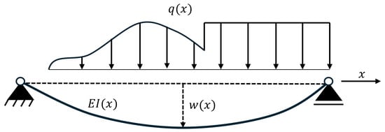
Figure 1.
Scheme showing variables of the general bending beam setup. Loading q and bending stiffness are arbitrary functions of coordinate x. The supports can be of various kinds.
The derivatives of contain the information about the beam slope, denoted by and the governing internal forces, namely the bending moment, , and the shear force, :
These equations contain the physical knowledge about the system to be analyzed and are considered within the loss function for the neural network training. In case of constant , the Euler–Bernoulli equation can be simplified as follows [30]:
Axial displacements are considered additionally to the bending deflection for each structural element. The differential equation for the corresponding tension bar is denoted as
where is the axial displacement, A is the cross-section area and the term is the axial load function over the length. denotes the internal axial forces. Figure 2 shows a rod with the corresponding load and displacement functions.
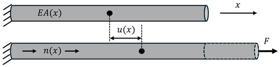
Figure 2.
Scheme showing variables for general rod setup. and the axial load n are general functions of the coordinate x.
For constant the differential equation simplifies to
In case of , the normal force in axial direction is constant and the first derivative of is sufficient to approximate the axial displacement
where F is a single axial force acting on the right side of the element as indicated in Figure 2.
2.2. Nondimensionalization
Data normalization is a common practice in traditional deep learning. It is a prerequisite processing step that involves scaling the input features of a dataset to obtain similar data magnitudes and ranges. However, this process is not generally applicable to physics problems, as the target solutions are typically not available and therefore it cannot be scaled. In the context of PINNs, it is imperative to ensure that the network outputs fall within a reasonable range. A common approach to ensure this is the nondimensionalization of the governing differential equation, a technique frequently employed in mathematics and physics [31]. Normalization and nondimensionalization are proven to enhance the training performance of neural networks by mitigating disparities in variable scales and improving convergence [6,32]. Nondimensionalization addresses problems with unstable network training due to differently scaled variables and is an effective method for enhancing training performance. The nondimensionalization of a differential equation involves the removal of all units from the equation and the uniform scaling of the variables.
First a constant bending stiffness of the beam is assumed. The Euler–Bernoulli equation’s independent variable is x and the two dependent variables are w and q. The physical parameters that are relevant to the problem are the length of the beam, denoted by L, and the bending stiffness . These parameters are selected as the characteristic scales. The dimensionless variables are defined as follows
The beam length, the beam slope, the bending moment and the shear force are not involved in nondimensionalizing the equation, but will be calculated as nondimensional quantities within the implementation:
Substituting the dimensionless variables into the differential equation yields to the following equation
which leads to the nondimensional form of the Euler–Bernoulli equation
The corresponding nondimensional slope, bending moment and shear force read
In case of non-constant bending stiffness, it is necessary to extend this equation by considering as a function of a given reference value :
The resulting nondimensional form of the Euler–Bernoulli equation for variable bending stiffness reads
The associated implementation considers the differential equation and its variables in their nondimensional form. The output quantities are re-dimensionalized in post-processing.
The governing equation for axial displacements with constant EA is nondimensionalized as follows:
with
2.3. Neural Network Architecture
Each beam component is represented by a neural network comprising only a single hidden layer. The network input is the normalized -coordinate, distributed along the length of the beam, and network output is the corresponding displacement value as shown in Figure 3.
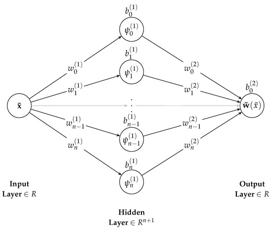
Figure 3.
Network architecture representing the bending deflections of a single beam on the nondimensional length scale . are the linear weights of the input and hidden layers of the network, and and are the corresponding biases and activation functions of the neurons.
The network utilizes the hyperbolic tangent function as its activation function in a single hidden layer. This network architecture is sufficient to model a smooth, one-dimensional displacement function along the beam’s length. The network parameters are initialized randomly from a standard Gaussian distribution, with a mean value of and a standard deviation of . The network acts as an approximation of the deflection curve of the beam for a given load. The network is trained by evaluating the mismatch of the differential Equations (13) and (14) evaluated at a given number of collocation points, which are distributed equidistant over the length of a beam. Additionally, the boundary conditions depending on the system configuration have to be considered in the loss function, which will be introduced in Section 2.5.
The derivatives of the neural network outputs are obtained via automatic differentiation, a computational technique that systematically applies the chain rule to a sequence of elementary operations, allowing for the exact and efficient calculation of gradients. By incorporating the differential equation directly into the training process, the neural network becomes physics-informed, which defines the essence of the PINN approach [1].
2.4. PINN-Framework for Coupled Elements with Beam and Axial Displacements
The modeling of frame structures with several coupled structural elements is realized by constructing separate networks for each beam and axial displacements. Thus, each structural element is represented by two feed-forward neural networks, one network models the behavior under a transverse load applying the Euler–Bernoulli equation and the second network models the behavior under an axial load, as described in Section 2.1. The two network types are defined as follows:
- PINNBEAM for capturing bending behavior (Euler–Bernoulli).
- PINNROD-A for capturing axial deformation, when .
- PINNROD-B for capturing axial deformation, when .
The PINNBEAM network is constructed as described in Section 2.3 by considering an arbitrary transverse load function . PINNROD-A and PINNROD-B are designed to approximate the axial displacements depending on the applied axial load. Here, two cases, one with constant axial load and the second without axial load, are considered. Within our study, we will focus on cases with constant axial load. Therefore, the PINNROD-A is defined as a feed-forward neural network with one hidden layer, employing a quadratic activation function
This assumption results in a quadratic network output as obtained for . PINNROD-B consists of only one hidden layer with a single linear neuron. The resulting displacement output is linear and will automatically result in . The presented framework can be extended in a similar manner to accommodate higher-order load functions for the axial loads, but we introduced this simplification due to efficiency reasons.
The training of all networks is performed in one system concurrently through a unified loss function, which incorporates all unknown parameters of all networks. The training procedure for a system with two elements is illustrated schematically in Figure 4 and the loss functions are discussed in detail in Section 2.5.
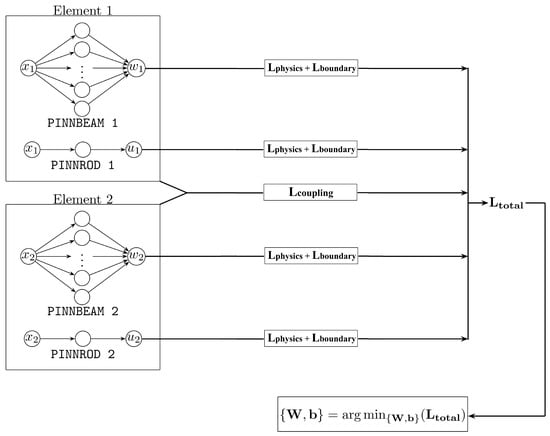
Figure 4.
PINN training scheme for an example structure with two elements by considering loss function terms for the physics for the boundary conditions for each element as well as for the coupling conditions between the two elements.
2.5. Loss Function
The loss function in a Physics-Informed Neural Network serves to penalize discrepancies between the neural network’s predictions and the governing physical laws, boundary conditions, and continuity requirements. It is essentially comprised of two components: the physics loss and the boundary condition loss. In instances where multiple elements are interconnected, an additional term that governs the transitional conditions is incorporated into the boundary condition loss. All loss terms described in the following are formulated using squared errors, which is simple to compute, differentiable, and strongly penalizes larger deviations, which enables the straight-forward application of gradient-based optimization methods.
2.5.1. Physics Loss
The physics loss term is responsible for ensuring that the final network output satisfies the underlying differential equations over the length of the beam. The physics loss is determined by calculating the PDEs residual, R, with respect to the approximated network output, and , at each collocation point . This is considered for the Euler–Bernoulli equation and the equation for axial displacements as follows:
The physics loss is subsequently determined by taking the mean squared residual over all collocation points :
These terms are finally weighted within the total physics loss
In the following study, the collocation points are defined equidistantly along each structural element. The influence of the number of points on the representation of the load and displacement functions is investigated in detail by means of the numerical examples.
2.5.2. Boundary Condition Loss
The boundary condition loss is contingent upon the system to be evaluated; distinct boundary conditions demand different derivatives of the network output. For a single structural element, the boundary condition loss consists of two beam components with two boundary conditions for each side of the beam and two rod components with one boundary condition for each side of the beam
where is the loss for the bending displacements and forces at the left side of the element at
and is the loss for the bending displacements and forces at the right side of the element at
and and are the corresponding losses for the axial displacements and forces
The exponents m,n,p,q,g, and h indicate the degree of the derivatives and might be different for the left and right side of the element and even for bending and axial displacements. The weights for bending and for axial boundary conditions have to be chosen carefully in order to ensure a certain accuracy of the boundary conditions without dominating the total loss function. In Table 1, the boundary conditions are formulated exemplary for different types of support conditions.

Table 1.
Boundary conditions for bending and axial displacements for different support types (adapted from [30]).
2.5.3. Coupling Condition Loss
In order to consider systems with multiple elements, it is necessary to incorporate additional coupling or transitional conditions into the loss function. These conditions guarantee that displacements, rotations, bending moments and internal forces remain continuous across the interfaces between connected structural elements. This ensures physical consistency and equilibrium in the overall system. The manner in which these elements are connected varies depending on the specific type of connection, such as a rigid corner or a moment joint connection. Since different elements are nondimensionalized with respect to their own reference parameters, the coupling requires transformation of the quantities of one element into the nondimensional space of the connected element. In Table 2, different examples are given for the coupling conditions of displacements and rotations, which define structural consistency, and force and bending moment conditions obtained by the equilibrium conditions.
Table 2.
Different examples for the connection of structural elements and the corresponding coupling conditions: (a) two beams with rigid connection, (b) two beams with hinged connection, (c) rigid corner with two elements, and (d) rigid corner with three elements.
In case (a), for the two beams with a rigid connection, both local coordinate systems align and the coupling conditions can be formulated in a straight-forward manner:
where , , and indicate the cross-section properties and length of the left beam and , , and are the properties of the right beam in the sketch.
When two structural elements are connected with an arbitrary angle, the displacement and force conditions must additionally account for the orientation of the elements in the global coordinate system. However, the rotational and moment conditions remain unchanged from Equation (24), since the moment is independent of the connection angle and the rotation is already defined relative to each element’s local orientation. If the elements are connected at a 90° angle, which is case (c) in Table 2, the displacement and force coupling conditions are considered as follows:
In the case of a connection different from 90° or 180°, equilibrium must still be enforced in the global coordinate system. This requires the transformation of the local force components of each element into the global coordinate system, in order to consistently combine all acting forces in the nodal equilibrium conditions.
In case that more than two elements are connected at a connection node, it is imperative that the equilibrium of moment and force is satisfied at that particular node. Consequently, it can be deduced that the moment and force transitional condition loss terms can also contain more than two terms. One example is case (d) in Table 2, which is investigated in one of the numerical examples. For this case, the coupling loss reads for the forces and moments as follows:
, , and indicate the properties of the left horizontal element, , , and define the properties of the right horizontal element, and , , and belong to the vertical element as indicated in case (d) in Table 2.
The weighted sum of all coupling loss terms provides the total coupling loss
The coupling condition loss is treated as part of the boundary condition loss in the optimization progress in Section 3. The summation of all loss terms finally yields the total loss function, which depends on all network parameters and serves as the objective to be minimized during the PINN training process
The weights must be selected carefully to ensure a balanced contribution from all transitional conditions, preventing any single term from dominating the loss and potentially impairing convergence or physical accuracy. In our study, we adjusted all weight factors manually. For the simple beam examples, all boundary loss weights were taken as one while the physics loss weights were increased to factor 10 in order to assure a sufficient representation of the differential beam equation. In case of multiple structural elements with bending and axial displacements, this selection is not straight forward and requires several manual iteration steps, especially for the coupling conditions. Here, further investigations on an automatic weight adjustment approach would be necessary.
2.6. Network Training
The objective of training the PINN is to identify one or more functions, each of which is represented by a neural network, that satisfy the corresponding differential equations and boundary conditions. In order to identify a function that fulfills this task, it is necessary to minimize the loss function, defined in Section 2.5, by seeking the optimal neural network parameters on the loss function space. Due to the complexity of the loss function for frame structures with multiple elements, the training process was implemented using the efficient PyTorch library [33], where the Adam optimizer [34] is commonly employed to perform gradient-based updates of the network parameters. For the investigated frame structures, learning rate schedulers were considered to facilitate convergence by systematically adjusting the learning rate as training progressed. In the final example, the optimization with ADAM converged quite slowly from a certain number of iterations, due to the large number of loss function terms. Here, a switch to the gradient-based L-BFGS algorithm was applied [35]. This approach combines the strengths of both optimizers, first leveraging ADAMs ability to avoid saddle points, which are dominating the loss landscape in PINN training, to get close to a local minimum and then use a second order method, which reduces the condition number for faster convergence [36]. However, the benchmarking of the different optimization algorithms is not the focus of the current study, but may be addressed in more detail in future work.
Further details on the network implementation, the setup of the training process, and extraction of the results can be found in the data archive mentioned in the Data Availability Statement of this paper.
3. Results
In this section, various structural examples are analyzed with the presented PINN approach. Within the first two examples, the convergence of the PINN solution is investigated with different number of collocation points and hidden neurons in each element. The boundary loss and the physics loss are considered with a default choice of the loss weights. The convergence of the finite element solution is investigated in comparison using standard Euler–Bernoulli beam elements without shear deformation [37]. Further details on this element type can be found in Appendix A. For the first two simple beam examples, the implementation of the PINN and FEM solution is realized using the MATLAB R2024b software package [38] with standard functionality.
Within the third and fourth example, the combination of several beam and rod elements including the coupling and boundary conditions is investigated. For both examples, the finite element solution is considered as reference solution whereby 20 Euler–Bernoulli beam elements are used to discretize each structural element of the structure using the software package Dlubal RSTAB 9 [39]. The PINN model was implemented within the PyTorch framework [33] as explained in the previous section. For these two examples, we put our focus on the consistency of the coupling and boundary conditions and we will use a fixed network setup of 10 hidden neurons and 101 collocation points.
All example implementations are available in the accompanying dataset mentioned in the data availability statement.
3.1. Cantilever Beam with Quadratic Load
In the first example, a cantilever beam with constant bending stiffness subjected to a quadratic load function as shown in Figure 5 is investigated. The corresponding beam properties are given in Table 3.
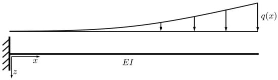
Figure 5.
Cantilever beam with constant bending stiffness subjected to a quadratic load .
Table 3.
System properties of the cantilever beam with quadratic load.
The beam was analyzed first with an increasing number of two-node Euler–Bernoulli beam elements as given in Appendix A. The degrees-of-freedom in x-direction were fixed within this example, which results in bending displacements only. The quadratic load was represented either with an element-wise constant load, which was assumed as the average load within the specific finite element, or an element-wise linear load function according to the nodal load table given in Table A1. In Figure 6, the representation of the analytical load function with the finite element model is shown for a discretization of three and six nodes. For the second case, the piece-wise linear element load is already quite close to original load function.
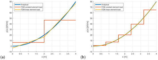
Figure 6.
Cantilever with quadratic load: approximation of defined load function with constant and linear element loads using (a) two elements and three nodes; (b) five elements and six nodes.
The corresponding displacements, slope, bending moments, and shear forces are shown in Figure 7 for the six-node discretization in comparison to the analytical solution obtained from the beam equations in Section 2.1. The FEM results are given in Table 4 by means of the maximum relative errors evaluated at every node i. This error measure is the maximum absolute value of the deviation of the estimated values and the analytical solution values normalized by the maximum absolute displacement value
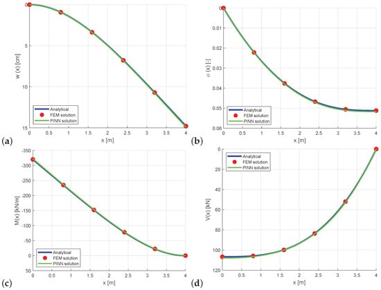
Figure 7.
Cantilever with quadratic load: comparison of FEM with six nodes and linear element loads with PINN solution using six collocation points and three hidden neurons for the (a) bending displacement , (b) slope , (c) bending moment , and (d) shear force .
Table 4.
Cantilever with quadratic load: comparison of maximum relative errors in displacement values , slope values , bending moments , shear forces and load values for finite elements with constant and linear element load and the PINN solution with different numbers of collocation points and hidden neurons.
The relative errors of the slope, bending moments, and shear forces given in Table 4 are calculated in the same manner. The table indicates a perfect convergence of the FEM results for constant and linear element loads with increasing node number.
The PINN accuracy was investigated next with different numbers of hidden neurons and collocation points. As activation function the hyberbolic tangent function was used. The PINN was implemented in the MATLAB software package [38]. The loss function was minimized using the MATLAB fminsearch function with a constant budget of 50.000 function evaluations. The training was repeated 10 times to reduce the influence of the scatter of the initial weights. The loss weighting factors were chosen manually as follows:
Figure 7 shows the PINN solution using six collocation points and three hidden neurons which agrees already quite well with the analytical solution. In Table 4, the obtained maximum relative errors of the PINN solutions are compared to the errors of the FEM solutions. Different configurations of collocations points and hidden neurons were investigated. The figure and the table indicate that, already for 3 hidden neurons, the displacement function could be already represented with a certain accuracy. Using 5 or 10 hidden neurons lead to the smallest errors in the beam results. On the other hand, increasing the number of hidden neurons to 15 or 20 did not lead to better results, which might by caused by the increasing number of unknown weights in the optimization procedure while the budget was fixed. However, the result show that using 5 or 10 hidden neurons, similar errors could be achieved if the number of collation points is chosen as 11 or higher. If the number of collocation points is chosen to small, overfitting phenomena may occur and may lead to wrong results between these points as shown in Figure 8.
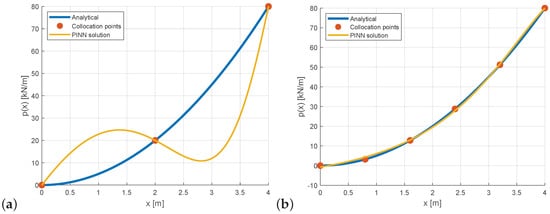
Figure 8.
Cantilever with quadratic load: PINN approximation of defined load function with (a) three collocation points and five hidden neurons, and (b) six collocation points and three hidden neurons.
The PINN solutions with 5 and 10 hidden neurons is more accurate for a given number of collocation points than the finite element solution with the same number of nodes if constant element loads are used. If the quadratic load is presented by element-wise linear loads, the finite element solution outperforms the PINN solution significantly. However, the PINN approach supports such a more sophisticated load function in a straight-forward manner, whereby the finite element approach requires the transformation of the load function to equivalent nodal load values, which is possible for specific function types only.
3.2. Cantilever Beam with Varying Bending Stiffness
In the second example, a cantilever beam with varying bending stiffness, as shown in Figure 9, is investigated. In this example, again, only bending displacements are considered according to Equation (13).
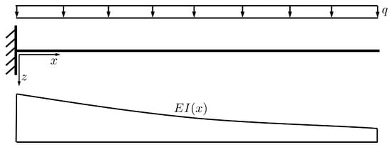
Figure 9.
Cantilever beam with constant load and decreasing bending stiffness .
The beam consists of structural steel with a given length L and a rectangular cross-section with width b and a linearly decreasing height . The corresponding beam properties and the assumed constant load is given in Table 5.
Table 5.
System properties of the cantilever beam with decreasing bending stiffness.
The bending stiffness under a linear height results in the following cubical function
with and .
The reference solution of the shear forces and bending moments are obtained analytically directly from the load function and the boundary conditions. The reference for the slope and the displacements was obtained from the bending moment and stiffness functions by numerical integration using the trapezoid rule with 500 discretization intervals. Again, the finite element solution with an increasing node number was investigated using the Euler–Bernoulli beam formulation given in Appendix A. The corresponding results are given in Table 6 which show again a clear convergence with increasing node number.
Table 6.
Cantilever with varying stiffness: comparison of maximum relative errors in displacement values , slope values , bending moments , shear forces , and load values for finite elements and the PINN solution with different numbers of collocation points.
The PINN solution was investigated similarly to the first example with an increasing number of collocation points. The number of hidden neurons has been selected from the findings of the first example. The PINN was implemented again in the MATLAB software package [38] and the loss function was minimized by the MATLAB fminsearch function with a constant budget of 50.000 function evaluations. For the calculation of the loss functions the beam formulation in Equation (13) has been considered. The resulting derivatives of the product were calculated by applying the product rule, combining the respective derivatives of and . The loss weighting factors for this example were chosen manually as follows:
The resulting beam displacements and the derived bending moment, shear forces, and approximated external load function are shown in Figure 10 and in Table 6. The results show an excellent agreement with the reference solutions, whereby a higher accuracy could be obtained as the finite element solution with a corresponding node number.
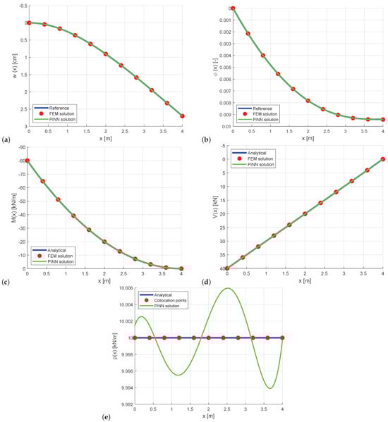
Figure 10.
Cantilever with varying stiffness: comparison of FEM with 11 nodes with the PINN solution using 11 collocation points and 5 hidden neurons for the (a) bending displacement , (b) slope , (c) bending moment , (d) shear force , and (e) approximation of load function .
3.3. T-Structure with Multiple Beams
As third example, the T-structure shown in Figure 11 is analyzed. The corresponding system properties are given in Table 7. This structures connects three individual beam elements, whereas the transverse and axial displacements are considered as unknowns for each member in the PINN approximation. Element one and two correspond to a standardized steel profile of type IPEa-270, and element three corresponds to a profile of type HEAA-220. Each element in this configuration is supported by a nodal support. The elements are rigidly connected, thereby ensuring that the global displacement and rotation of all elements are identical at the connection. Furthermore, the force and moment equilibrium must be satisfied at this point.
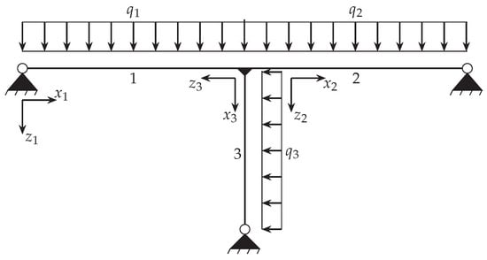
Figure 11.
T-structure consisting of three beam elements.
Table 7.
System properties of the T-structure with multiple beams.
The finite element solution using the software package Dlubal RSTAB 9 [39] is used as reference, whereas 20 Euler–Bernoulli beam elements are used to discretize each of the 3 beams of the structure. The finite element solutions are shown in Figure 12, Figure 13 and Figure 14 using the software package STRIAN 2.1 [40] for the plots.
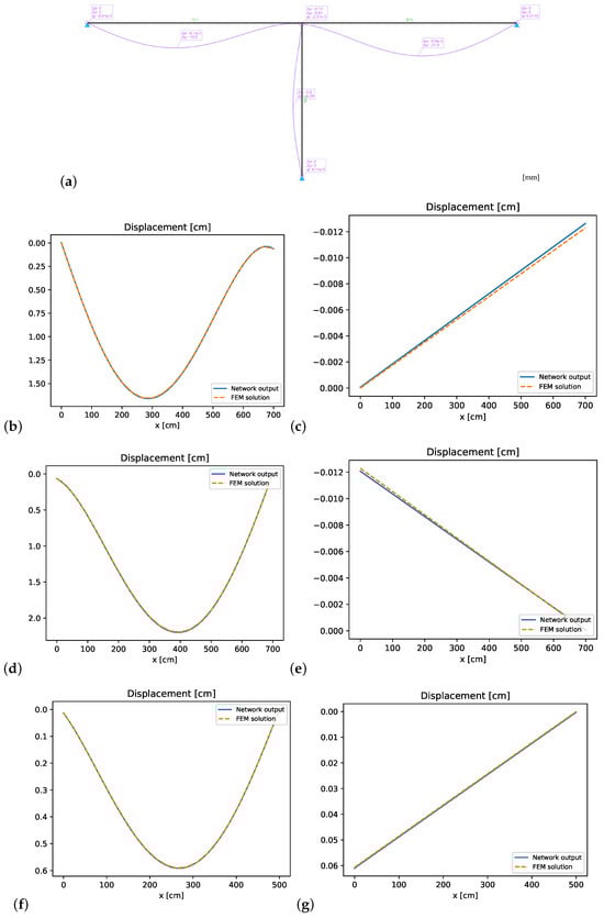
Figure 12.
T-structure: (a) FEM reference solution for displacements, and comparison with PINN results: (b) bending displacements element 1, (c) axial displacements element 1, (d) bending displacements element 2, (e) axial displacements element 2, (f) bending displacements element 3, and (g) axial displacements element 3.
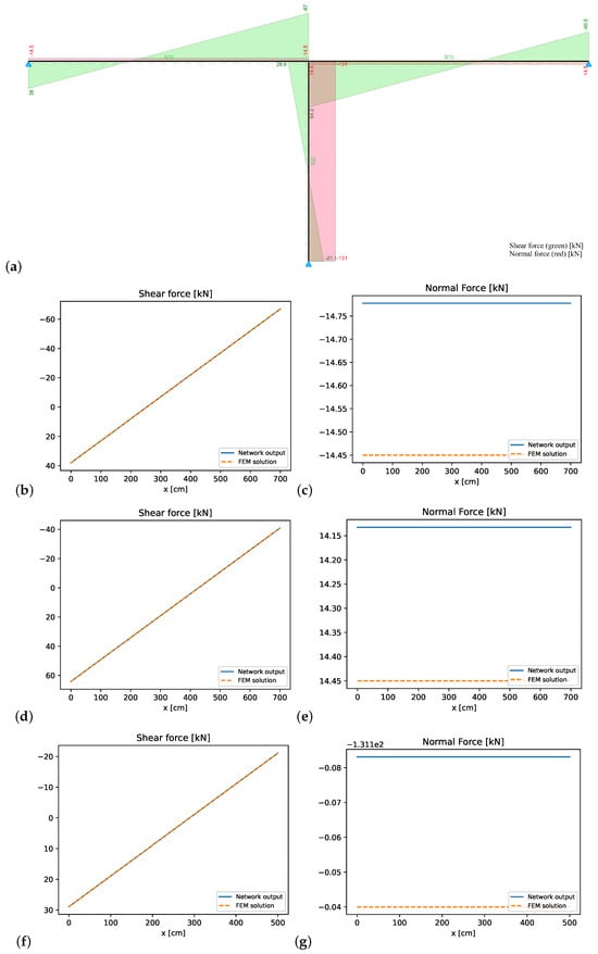
Figure 13.
T-structure: (a) FEM reference solution for shear and normal forces, and comparison with PINN results: (b) shear forces element 1, (c) normal forces element 1, (d) shear forces element 2, (e) normal forces element 2, (f) shear forces element 3, and (g) normal forces element 3.
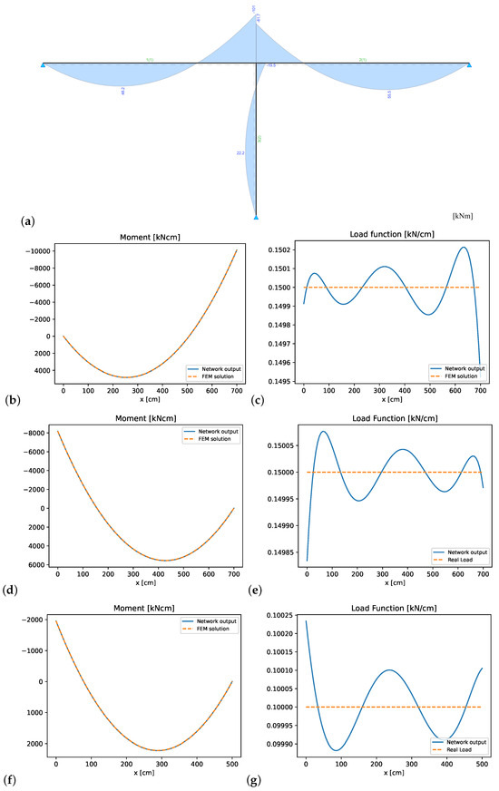
Figure 14.
T-structure: (a) FEM reference solution for bending moments, and comparison with PINN bending moments and load functions: (b) bending moment element 1, (c) load function element 1, (d) bending moment element 2, (e) load function element 2, (f) bending moment element 3, and (g) load function element 3.
The PINN-framework was designed according to the principles delineated in Section 2.4. Every structural element was represented by a PINNBEAM network with 10 hidden neurons to approximate the bending and a PINNROD-B network with 1 hidden neuron to approximate the axial displacements. The Adam optimization algorithm was utilized for the training using a reduce-on-plateau learning rate scheduler to ensure stable and efficient convergence. The loss weighting factors were manually adjusted using similar values for the same type for all elements k. For the physics contributions, the weight factors were set to
the boundary condition terms were weighted by
and weights for the coupling conditions were set to
Figure 12, Figure 13 and Figure 14 present the results for the individual structural elements. The network outputs for both bending displacements and axial deformations closely match the reference solution across all structural elements. However, small deviations could be observed for the axial displacements and normal forces. The increase in the corresponding weights could reduce these errors. The same behavior could be observed for the coupling conditions: while the bending displacements and moments agree very well with the reference, the axial displacements and forces required special attention within the loss weighting. However, the investigated PINN approach can handle multiple interacting elements while preserving continuity and equilibrium across the connections, but the adjustment of the weighting factors is the crucial point and requires additional manual tuning effort.
The convergence behavior of the optimizer is shown in Figure 15 and indicates a stable progress, interspersed with multiple jumps as the optimizer explores different local minima in the loss landscape. Overall, training remains stable, and optimization is terminated after 25,000 epochs.
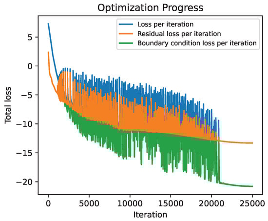
Figure 15.
Optimization convergence history of the logarithmic total loss for the T-structure.
3.4. Double-Hinged Frame
In the final example, a double-hinged frame composed from three different elements as shown in Figure 16 is investigated. The columns, elements 1 and 3 are supported by pinned supports, while the horizontal beam element 2 is rigidly connected to both columns at a 90° angle. The properties of the three elements are given in Table 8, whereby for the columns, a profile of type HEAA-220 was chosen and for the horizontal beam, an IPEa-270 was selected.
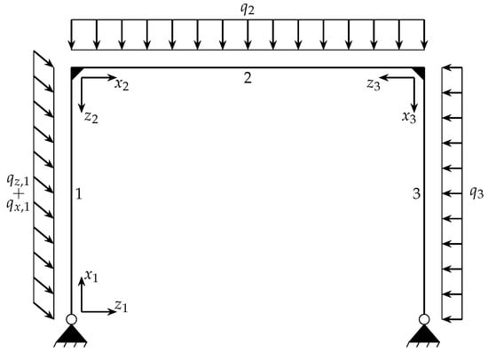
Figure 16.
Double-hinged frame structure.
Table 8.
System properties of the double-hinged frame structure.
Again, the finite element solution using the Dlubal software package with 20 elements per beam and column are used as reference. The finite element solution is shown in Figure 17, Figure 18 and Figure 19 using the software package STRIAN 2.1 for the plots.
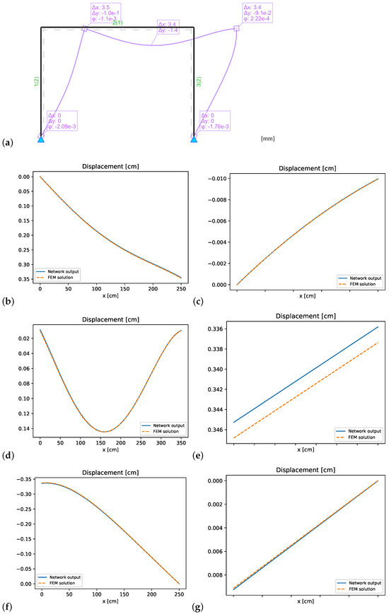
Figure 17.
Double-hinged frame: (a) FEM reference solution for displacements, and comparison with PINN results: (b) bending displacements element 1, (c) axial displacements element 1, (d) bending displacements element 2, (e) axial displacements element 2, (f) bending displacements element 3, and (g) axial displacements element 3.
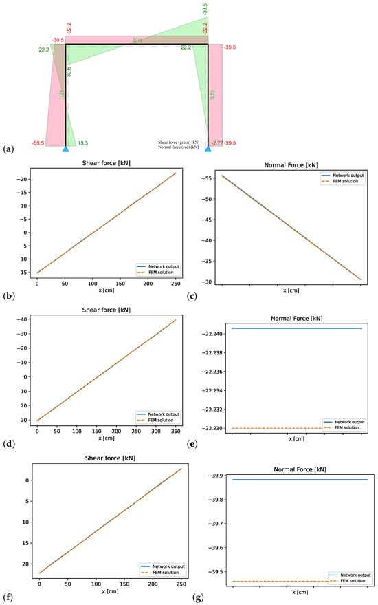
Figure 18.
Double-hinged frame: (a) FEM reference solution for shear and normal forces, and comparison with PINN results: (b) shear forces element 1, (c) normal forces element 1, (d) shear forces element 2, (e) normal forces element 2, (f) shear forces element 3, and (g) normal forces element 3.
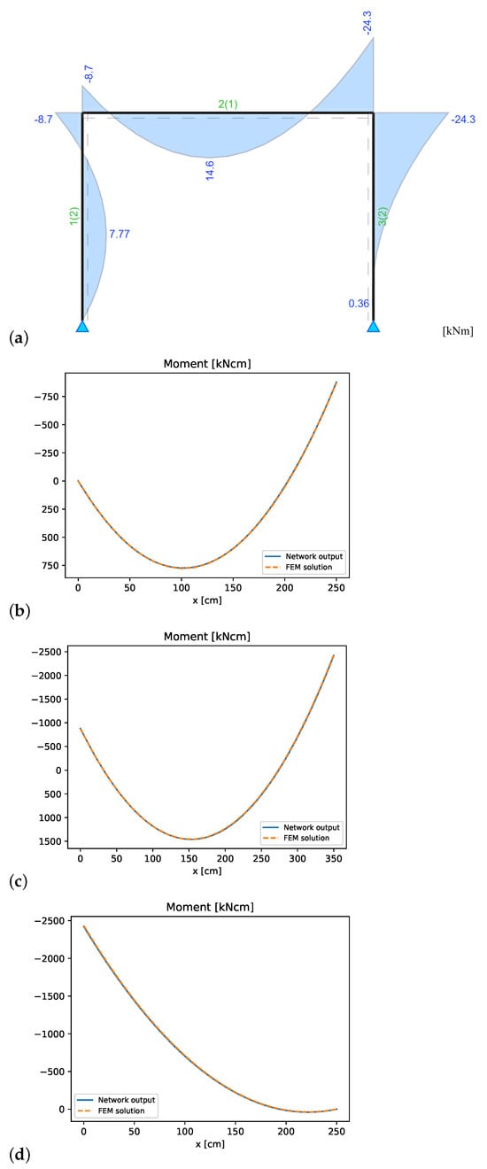
Figure 19.
Double-hinged frame: (a) FEM reference solution for bending moments, and comparison with PINN results: (b) element 1, (c) element 2, and (d) element 3.
The PINN-framework employed to solve this example also followed the principles delineated in Section 2.4. Every element was described by a PINNBEAM network with 10 hidden neurons to model the elements’ bending behavior. Since a constant axial load is acting on element 1, its axial displacements were modeled by a PINNROD-A network with three hidden neurons. Elements 2 and 3 were described by a PINNROD-B network with one hidden neuron to model the axial displacements. The optimization algorithm employed for this task was a combination of an Adam optimization followed by a L-BFGS optimization to ensure good convergence.
Figure 17, Figure 18, Figure 19 and Figure 20 show the results for this example. The PINN approximation sufficiently captures the axial and bending deformations, and the presence of the axial line load was handled effectively within the framework. The method successfully enforces all transitional conditions at the connecting nodes and satisfies the respective boundary conditions for the system. However, similar to the previous example, it was observed that the PINN’s performance is highly sensitive to the choice of loss weights. Small changes in these weights had a noticeable impact on convergence and final accuracy. This highlights the importance of proper weight selection and suggests that future work should consider automated strategies for dynamically tuning loss weights during training. Again, the loss weighting factors were manually adjusted using similar values for the same type for all elements k. For the physics contributions, the weights were set to
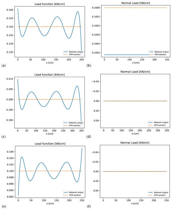
Figure 20.
Double-hinged frame: PINN load function results: (a) transverse load element 1, (b) axial load element 1, (c) transverse load element 2, (d) axial load element 2, (e) transverse load element 3, and (f) axial load element 3.
The boundary condition terms were weighted by
The weights for the coupling conditions were generally set to
Additionally, four specific force conditions required significantly higher weighting to obtain a stable and accurate solution. In particular, the conditions enforcing equilibrium between the shear force at the end of element 1 and the normal force at the start of element 2, as well as between the normal force of element 2 and the shear force of element 3; these conditions were weighted with
Similarly, the conditions ensuring continuity between the normal force at the end of element 1 and the shear force at the start of element 2, as well as between the shear force at the end of element 2 and the normal force at the start of element 3, were weighted with
Figure 21 shows the optimization progress over 25,000 training epochs. For the first 17,000 epochs, the optimizer exhibits stable behavior while gradually exploring and minimizing the loss landscape. During this phase, both the physics and boundary condition losses decrease steadily. However, beyond 17,000 epochs, the optimization becomes increasingly unstable, with noticeable fluctuations in the total and component losses. This instability reflects the optimizer struggling to further minimize the loss or settling into local minima. At exactly 25,000 epochs, the optimization method is switched from Adam to L-BFGS, which leads to the prominent spike in the total loss observed at the end of the graph. This switch aims to refine the solution and improve convergence in the final training phase.
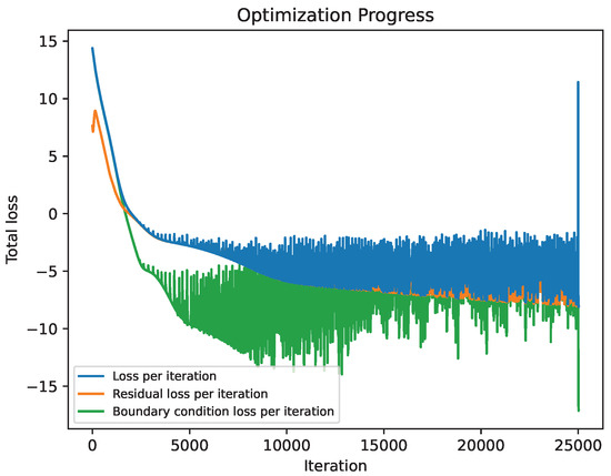
Figure 21.
Optimization convergence history of the logarithmic total loss for the double-hinged frame.
4. Discussion
In the first part of this study, the accuracy of FEM and PINN solutions for special cantilever type problems with pure bending under Euler–Bernoulli theory were evaluated. The maximum deviation of deflection, slope, bending moment, and shear forces were evaluated for identical number of nodes in the FE discretization and number of collocation points in the PINN model. For a prismatic beam subjected to a quadratic load, the PINN method offered higher accuracy compared to FEM with piecewise constant load approximation but is inferior once the load is implemented with piecewise linear functions. For the case of a beam with varying bending stiffness under uniform loading, the PINN also shows slightly lower deviations in the deflections and slope values . One should also consider, that for the evaluation of FEM accuracy, only the respective values at the nodes were used, while the PINN accuracy relates to a continuous solution, which can be evaluated at any point without additional computational efforts.
Subsequently, two 2D frame structures, which consists of three structural elements, were analyzed with the presented PINN approach. The displacements in transverse and axial directions for each element were modeled separately by a single neural network with a single hidden layer. The investigations could show that the obtained approximation was sufficiently accurate to represent the resulting internal forces and displacement functions. The coupling conditions between two or more elements and the boundary conditions at the supports of the structure were imposed in a joined loss function for the training procedure by specific weighting factors. These weights were chosen by hand and were found to have a substantial influence on the convergence behavior and final accuracy of the trained networks, pointing at the necessity of sophisticated loss balancing for more complex structures. Especially, the consideration of the axial displacements and forces in the rigid corners increased the manual effort to obtain optimal weighting factors.
It is imperative to acknowledge that while the presented optimization strategies led to satisfactory results, they are not guaranteed to be optimal. It is noteworthy that different training schemes and hyper-parameter configurations may yield improved performance, and the approaches adopted in this study were chosen based on empirical observations rather than exhaustive tuning.
There are several possible improvements already tested in existing research that could be implemented into our framework in future work for a more reliable convergence and higher accuracy of the results. The sensitivity of the latter with respect to the weighting terms in the loss function has reinforced the necessity for automatizing the choice of these values. This can be conducted by updating the weight terms together with the network parameters according to loss gradients [31] or by adding weights as trainable parameters [41]. Alternatively, augmented Lagrangian methods can be employed for adaptive loss-balancing, which was proven to be superior to the standard penalty method for training PINNs [42]. This study further implemented equidistant placement of collocation points, which disregards particularities of the solution. In case of sudden changes of cross-sectional parameters or the loading along the beam elements and for improved accuracy around joints, an adaptive sampling strategy, which can be based on, e.g., the local residual [43,44], could improve the flexibility and convergence of our framework with respect to different element shapes and loading conditions.
The presented approach assumes a continuous displacement function including all derivatives up to fourth order. In case of single force or moment loads acting inside the domain of a single structural element, the resulting discontinuity can not be represented sufficiently well with the continuous approximation function. For such cases, it is recommended to split each structural element at any discontinuity due to loading or cross-section properties.
5. Conclusions
For the cantilever beam use cases with spatially varying cross-section parameters and loading conditions, the PINN method can effectively leverage the explicit implementation of their analytical form to provide slightly more accurate results than the FEM. For the considered frame structures, our PINN framework was able to accurately capture the coupling of axial and bending deformation of multiple members. Convergence of the optimization was way less reliable compared to single member treatment and highly sensitive to the scaling of coupling conditions in the loss function. In its current form, the presented approach can only be considered complementary to the well-established FEM and seen as a first step towards building a general framework for solving large general frame structures. Future work will focus on improving the optimization procedure with automatized loss balancing and collocation sampling methods towards more reliable accuracy. Thereupon, a systematic quantitative comparison with FEM accuracy for a broad range of frame architectures will be necessary. For the proof of concept, the considered frame structures in this study were limited to specific coupling angles; however, we expect the method to work for arbitrary angles, which only requires a flexible adaptation of the coupling of axial and transverse terms. We also aim to implement the option of adding shear effects by means of Timoshenko beam theory or even extend the framework from 2D to 3D applications, where additionally torsional effects could be considered with, e.g., a complete linear expansion case [45].
After establishing a reliable framework for linear elastic analysis, an extension to nonlinear problems might be thinkable. Approaches for treating material nonlinearity such as cracking reinforced concrete [46], perfect plasticity [47], or hyperelasticity [48], but also geometric nonlinearity [49] already exist in the framework of PINNs, but require more complex network structures and will pose additional challenges for reliable optimization. Building on results from [5,6], our framework could even be used for time-dependent loading conditions and vibration analysis of frame structures.
Author Contributions
Conceptualization, L.L. and T.M.; methodology, F.D., L.L. and T.M.; software, F.D., L.L. and T.M.; validation, F.D., L.L. and T.M.; formal analysis, F.D. and T.M.; investigation, F.D. and T.M.; resources, F.D. and T.M.; data curation, F.D.; writing—original draft preparation, F.D.; writing—review and editing, L.L., T.M. and C.K.; visualization, F.D. and T.M.; supervision, L.L., T.M. and C.K.; project administration, T.M.; funding acquisition, C.K. All authors have read and agreed to the published version of the manuscript.
Funding
This research has been supported by the German Research Foundation (DFG) through the project DIVING within the priority program SPP 100+.
Institutional Review Board Statement
Not applicable.
Informed Consent Statement
Not applicable.
Data Availability Statement
The complete calculation files including all presented results are available in the publicly accessible repository https://refodat.de/receive/refodat_mods_00000058 (assessed on 18 November 2025).
Conflicts of Interest
The authors declare no conflicts of interest.
Abbreviations
The following abbreviations are used in this manuscript:
| PDE | Partial differential equation |
| ML | Machine learning |
| NN | Neural network |
| ANN | Artifical neural network |
| FEM | Finite element method |
| PINN | Physics-informed neural network |
| ADAM | Adaptive Moment Estimation |
| L-BFGS | Limited-memory Broyden–Fletcher–Goldfarb–Shanno |
Appendix A
The standard finite element using a Euler–Bernoulli beam formulation considers two nodes each having two displacement and one rotational degrees-of-freedom as shown in Figure A1.

Figure A1.
Finite element with local coordinate system and corresponding displacement and rotational degrees-of-freedom.
If element loads are neglected, cubic interpolation functions for the bending and linear interpolation for the axial displacements are sufficient to represent the underlying differential equations exactly [50]
The corresponding stiffness matrix of one finite element in local coordinates reads for constant cross-section properties as follows [37]
The matrix entries for bending displacements and rotations are decoupled from the axial displacement entries as introduced in Section 2.1 only for geometrical linear element formulations.
If element loads should be considered, they have to be transformed to nodal loads for specific loading conditions as discussed in [37]. Within our study, only constant and linear load representations are applied. The corresponding nodal loads are given in Table A1.
Table A1.
Nodal loads for constant and linear element loads according to [37].
Table A1.
Nodal loads for constant and linear element loads according to [37].
| Load | Normal Loads | Shear Loads | Moment Loads |
|---|---|---|---|
| Constant | |||
| Linear | |||
| Constant | |||
References
- Raissi, M.; Perdikaris, P.; Karniadakis, G. Physics-informed neural networks: A deep learning framework for solving forward and inverse problems involving nonlinear partial differential equations. J. Comput. Phys. 2019, 378, 686–707. [Google Scholar] [CrossRef]
- Karniadakis, G.E.; Kevrekidis, I.G.; Lu, L.; Perdikaris, P.; Wang, S.; Yang, L. Physics-informed machine learning. Nat. Rev. Phys. 2021, 3, 422–440. [Google Scholar] [CrossRef]
- Cuomo, S.; Di Cola, V.S.; Giampaolo, F.; Rozza, G.; Raissi, M.; Piccialli, F. Scientific machine learning through physics–informed neural networks: Where we are and what’s next. J. Sci. Comput. 2022, 92, 88. [Google Scholar] [CrossRef]
- Bai, J.; Rabczuk, T.; Gupta, A.; Alzubaidi, L.; Gu, Y. A physics-informed neural network technique based on a modified loss function for computational 2D and 3D solid mechanics. Comput. Mech. 2023, 71, 543–562. [Google Scholar] [CrossRef]
- Fallah, A.; Aghdam, M.M. Physics-informed neural network for bending and free vibration analysis of three-dimensional functionally graded porous beam resting on elastic foundation. Eng. Comput. 2024, 40, 437–454. [Google Scholar] [CrossRef]
- Kapoor, T.; Wang, H.; Núñez, A.; Dollevoet, R. Physics-informed neural networks for solving forward and inverse problems in complex beam systems. IEEE Trans. Neural Netw. Learn. Syst. 2023, 35, 5981–5995. [Google Scholar] [CrossRef]
- Al-Adly, A.I.; Kripakaran, P. Physics-informed neural networks for structural health monitoring: A case study for Kirchhoff–Love plates. Data-Centric Eng. 2024, 5, e6. [Google Scholar] [CrossRef]
- Lippold, L.; Rödiger, N.; Most, T.; Könke, C. Identifikation inhomogener Materialeigenschaften von Flächentragwerken mit Physics Informed Neural Networks. In Proceedings of the 15. Fachtagung Baustatik–Baupraxis, Hamburg, Germany, 4–5 March 2024. [Google Scholar]
- Guo, H.; Zhuang, X.; Rabczuk, T. A deep collocation method for the bending analysis of Kirchhoff plate. arXiv 2021, arXiv:2102.02617. [Google Scholar] [CrossRef]
- Xu, C.; Cao, B.T.; Yuan, Y.; Meschke, G. Transfer learning based physics-informed neural networks for solving inverse problems in engineering structures under different loading scenarios. Comput. Methods Appl. Mech. Eng. 2023, 405, 115852. [Google Scholar] [CrossRef]
- Bastek, J.H.; Kochmann, D.M. Physics-informed neural networks for shell structures. Eur. J. -Mech.-A/Solids 2023, 97, 104849. [Google Scholar] [CrossRef]
- Hu, H.; Qi, L.; Chao, X. Physics-informed Neural Networks (PINN) for computational solid mechanics: Numerical frameworks and applications. Thin-Walled Struct. 2024, 205, 112495. [Google Scholar] [CrossRef]
- Kamali, A.; Sarabian, M.; Laksari, K. Elasticity imaging using physics-informed neural networks: Spatial discovery of elastic modulus and Poisson’s ratio. Acta Biomater. 2023, 155, 400–409. [Google Scholar] [CrossRef]
- Zhang, E.; Yin, M.; Karniadakis, G.E. Physics-informed neural networks for nonhomogeneous material identification in elasticity imaging. arXiv 2020, arXiv:2009.04525. [Google Scholar] [CrossRef]
- Guo, X.Y.; Fang, S.E. Structural parameter identification using physics-informed neural networks. Measurement 2023, 220, 113334. [Google Scholar] [CrossRef]
- Abueidda, D.W.; Koric, S.; Al-Rub, R.A.; Parrott, C.M.; James, K.A.; Sobh, N.A. A deep learning energy method for hyperelasticity and viscoelasticity. Eur. J. -Mech.-A/Solids 2022, 95, 104639. [Google Scholar] [CrossRef]
- Haghighat, E.; Abouali, S.; Vaziri, R. Constitutive model characterization and discovery using physics-informed deep learning. Eng. Appl. Artif. Intell. 2023, 120, 105828. [Google Scholar] [CrossRef]
- Zheng, B.; Li, T.; Qi, H.; Gao, L.; Liu, X.; Yuan, L. Physics-informed machine learning model for computational fracture of quasi-brittle materials without labelled data. Int. J. Mech. Sci. 2022, 223, 107282. [Google Scholar] [CrossRef]
- Mai, H.T.; Lee, S.; Kang, J.; Lee, J. A damage-informed neural network framework for structural damage identification. Comput. Struct. 2024, 292, 107232. [Google Scholar] [CrossRef]
- Zhang, Z.; Sun, C. Structural damage identification via physics-guided machine learning: A methodology integrating pattern recognition with finite element model updating. Struct. Health Monit. 2021, 20, 1675–1688. [Google Scholar] [CrossRef]
- Grossmann, T.G.; Komorowska, U.J.; Latz, J.; Schönlieb, C.B. Can physics-informed neural networks beat the finite element method? Ima J. Appl. Math. 2024, 89, 143–174. [Google Scholar] [CrossRef]
- Meethal, R.E.; Kodakkal, A.; Khalil, M.; Ghantasala, A.; Obst, B.; Bletzinger, K.U.; Wüchner, R. Finite element method-enhanced neural network for forward and inverse problems. Adv. Model. Simul. Eng. Sci. 2023, 10, 6. [Google Scholar] [CrossRef]
- Hu, Z.; Shukla, K.; Karniadakis, G.E.; Kawaguchi, K. Tackling the curse of dimensionality with physics-informed neural networks. Neural Netw. 2024, 176, 106369. [Google Scholar] [CrossRef]
- Gere, J.; Timoshenko, S. Mechanics of Materials; PWS: Boston, MA, USA, 1997. [Google Scholar]
- Alkunte, S.; Fidan, I.; Naikwadi, V.; Gudavasov, S.; Ali, M.A.; Mahmudov, M.; Hasanov, S.; Cheepu, M. Advancements and Challenges in Additively Manufactured Functionally Graded Materials: A Comprehensive Review. J. Manuf. Mater. Process. 2024, 8, 23. [Google Scholar] [CrossRef]
- Gartia, A.; Chakraverty, S. Advanced computational modeling and mechanical behavior analysis of multi-directional functionally graded nanostructures: A comprehensive review. Comput. Model. Eng. Sci. 2025, 142, 2405. [Google Scholar] [CrossRef]
- Timoshenko, S.P. LXVI. On the correction for shear of the differential equation for transverse vibrations of prismatic bars. Lond. Edinb. Dublin Philos. Mag. J. Sci. 1921, 41, 744–746. [Google Scholar] [CrossRef]
- Iandiorio, C.; Milani, D.; Salvini, P. Optimal uniform strength design of frame and lattice structures. Comput. Struct. 2024, 301, 107430. [Google Scholar] [CrossRef]
- Faroughi, S.; Darvishi, A.; Rezaei, S. On the order of derivation in the training of physics-informed neural networks: Case studies for non-uniform beam structures. Acta Mech. 2023, 234, 5673–5695. [Google Scholar] [CrossRef]
- Meskouris, K.; Hake, E. Statik der Stabtragwerke, 2nd ed.; Springer: Berlin/Heidelberg, Germany, 2009. [Google Scholar]
- Wang, S.; Sankaran, S.; Wang, H.; Perdikaris, P. An Expert’s Guide to Training Physics-informed Neural Networks. arXiv 2023, arXiv:2308.08468. [Google Scholar]
- Yu, J.; Spiliopoulos, K. Normalization effects on deep neural networks. arXiv 2022, arXiv:2209.01018. [Google Scholar] [CrossRef]
- Paszke, A.; Gross, S.; Massa, F.; Lerer, A.; Bradbury, J.; Chanan, G.; Killeen, T.; Lin, Z.; Gimelshein, N.; Antiga, L.; et al. PyTorch: An Imperative Style, High-Performance Deep Learning Library. In Advances in Neural Information Processing Systems 32; Curran Associates, Inc.: San Francisco, CA, USA, 2019; pp. 8024–8035. Available online: http://papers.neurips.cc/paper/9015-pytorchan-imperative-style-high-performance-deep-learning-library.pdf (accessed on 18 November 2025).
- Kingma, D.P.; Ba, J. Adam: A Method for Stochastic Optimization. arXiv 2015, arXiv:1412.6980. [Google Scholar]
- Liu, D.C.; Nocedal, J. On the limited memory BFGS method for large scale optimization. Math. Program. 1989, 45, 503–528. [Google Scholar] [CrossRef]
- Rathore, P.; Lei, W.; Frangella, Z.; Lu, L.; Udell, M. Challenges in training pinns: A loss landscape perspective. arXiv 2024, arXiv:2402.01868. [Google Scholar] [CrossRef]
- Krätzig, W.; Harte, R.; Könke, C.; Petryna, Y. Tragwerke 2, 5th ed.; Springer Vieweg: Berlin, Germany, 2019. [Google Scholar]
- The MathWorks Inc. MATLAB User Documentation, R2024b ed.; The MathWorks Inc.: Natick, MA, USA, 2024; Available online: https://www.mathworks.com (accessed on 18 November 2025).
- Dlubal Software GmbH. RSTAB 9—User’s Manual: Modeling and Calculation of Beam, Frame, and Truss Structures, Version 9 ed.; Dlubal Software GmbH: Tiefenbach, Germany, 2025; Available online: https://www.dlubal.com/en/downloads-andinformation/documents/online-manuals/rstab-9 (accessed on 18 November 2025).
- Stibor, M.; Frantik, P. STRIAN—Structural Analyser, 2.1 ed.; Brno University: Brno, Czech Republic, 2020; Available online: https://structural-analyser.com/domains/www/online-free-structural-analysis.html (accessed on 18 November 2025).
- McClenny, L.D.; Braga-Neto, U.M. Self-adaptive physics-informed neural networks. J. Comput. Phys. 2023, 474, 111722. [Google Scholar] [CrossRef]
- Son, H.; Cho, S.W.; Hwang, H.J. Enhanced physics-informed neural networks with augmented Lagrangian relaxation method (AL-PINNs). Neurocomputing 2023, 548, 126424. [Google Scholar] [CrossRef]
- Wight, C.L.; Zhao, J. Solving Allen-Cahn and Cahn-Hilliard equations using the adaptive physics informed neural networks. arXiv 2020, arXiv:2007.04542. [Google Scholar] [CrossRef]
- Hou, J.; Li, Y.; Ying, S. Enhancing PINNs for solving PDEs via adaptive collocation point movement and adaptive loss weighting. Nonlinear Dyn. 2023, 111, 15233–15261. [Google Scholar] [CrossRef]
- Carrera, E.; Giunta, G.; Petrolo, M. Beam Structures: Classical and Advanced Theories; John Wiley & Sons: Hoboken, NJ, USA, 2011. [Google Scholar]
- Balmer, V.M.; Kaufmann, W.; Kraus, M.A. Physics-informed neural networks for nonlinear analysis of reinforced concrete beams. In Proceedings of the International Probabilistic Workshop, Guimarães, Portugal, 8–10 May 2024; pp. 271–280. [Google Scholar]
- Haghighat, E.; Raissi, M.; Moure, A.; Gomez, H.; Juanes, R. A physics-informed deep learning framework for inversion and surrogate modeling in solid mechanics. Comput. Methods Appl. Mech. Eng. 2021, 379, 113741. [Google Scholar] [CrossRef]
- Zhang, E.; Dao, M.; Karniadakis, G.E.; Suresh, S. Analyses of internal structures and defects in materials using physics-informed neural networks. Sci. Adv. 2022, 8, eabk0644. [Google Scholar] [CrossRef]
- Chen, L.; Zhang, H.Y.; Ouyang, W.; Liu, S.W. Implementation of physics informed neural networks for geometrically nonlinear analysis of non-prismatic members. In Proceedings of the Structures, Phoenix, AZ, USA, 9–11 April 2025; Volume 71, p. 108149. [Google Scholar]
- Chopra, A. Dynamics of Structures, 5th ed.; Pearson Education, Inc.: Uttar Pradesh, India, 2017. [Google Scholar]


Disclaimer/Publisher’s Note: The statements, opinions and data contained in all publications are solely those of the individual author(s) and contributor(s) and not of MDPI and/or the editor(s). MDPI and/or the editor(s) disclaim responsibility for any injury to people or property resulting from any ideas, methods, instructions or products referred to in the content. |
© 2025 by the authors. Licensee MDPI, Basel, Switzerland. This article is an open access article distributed under the terms and conditions of the Creative Commons Attribution (CC BY) license (https://creativecommons.org/licenses/by/4.0/).