1. Introduction
In 1952, Marcos Moshinsky published a seminal article entitled ‘Transient Phenomena in Quantum Mechanics: Diffraction in Time’ [
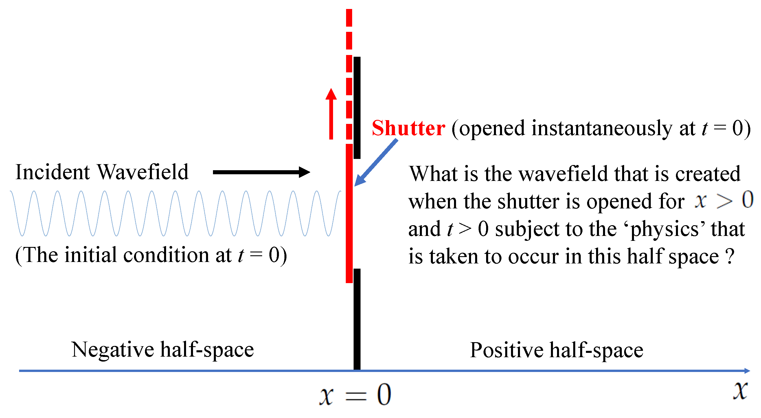
1]. Using a one-dimensional model, Moshinsky considered the case when a beam of non-relativistic electrons (travelling from left to right in the negative half-space) is incident upon a shutter (placed at
) so that they cannot propagate through to the positive half-space. At a time
, the shutter in opened instantaneously so that the electron beam can propagate through from the negative to the positive half-space. The problem is to evaluate the probability density of the resulting wave-function (determined by the Schrödinger equation) in the positive half-space as a function of both space and time. In other words, if
is taken to be the electron wave-field, then what is the
map, for
and
of
when the shutter is opened at
?
The space-time characteristics of the probability density are governed by the initial condition
of the field at
, where
is taken to represent of the electron beam in the negative half-space. In this context, the study undertaken by Moshinsky was an example of a control problem in quantum mechanics. The analysis undertaken by him involved developing a Green’s function solution to the homogeneous time-dependent Schrödinger equation [
2]. For atomic units (where the Dirac constant and the electron mass are set to 1), this equation is identical to the homogeneous time-dependent diffusion equation for a Diffusivity of
but with imaginary time. Consequently, the Green’s function for the time-dependent diffusion equation (for a Diffusivity of
), which includes the function
, yields a solution to the Schrödinger equation, which is characterised by the function
.
For a fixed value of
t, this is a ‘chirp function’ of space (a linear frequency modulated chirp with a ‘chirp parameter’ of
). It is therefore analogous to the convolution kernel associated with Fresnel diffraction [
3] which is characterised by a quadratic phase factor [
4]. However, for a fixed value of
x, as
, the function
oscillates at an increasingly high frequency, characterised by an inverse phase factor of time. For this reason, the phenomenon has been referred to as ‘Diffraction in Time’ (or even ‘Time Scattering’) [
5,
6]. The principal point here is that, unlike the diffusion equation, the same Green’s function solution applied to the Schrödinger equation yields a fundamentally different result, which is compounded in the oscillations of the wave-field in space but also, and, more significantly, in time.
The exact nature of these Fresnel-type oscillations depends on the initial condition, but the fact that such oscillations in time occur at all is due entirely to the characteristics of the Green’s function alone. This result illustrates a fundamental physical phenomenon, namely that a stream of electrons described by a plane wave-function with a fixed frequency, will spontaneously undergo rapid oscillations in time as soon as the shutter is opened. While such oscillations decrease in frequency (and amplitude) over time, the result shows that the electron wave-field spontaneously oscillates, due to the instantaneous opening of the shutter alone (with no other physical interactions). Such a transient phenomenon is now recognised as being a ubiquitous phenomenon in quantum dynamics [
7,
8], and, some fifty years after Moshinsky proposed such a dynamic process on theoretical grounds alone, experimental confirmation of the phenomenon was provided in 1996 using ultra-cold atoms [
9].
The experimental verification of the ‘Quantum Shutter Problem’, as it has come to be known, has led to a number of publications which have looked into the evaluation of the problem in three dimensions [
10], general formulations [
11], new theories of diffraction in time [
12], and an extension of the problem to include relativistic effects for both spin-less and half-spin particle beams [
13].
There are numerous applications to which fractional calculus is becoming a central theme [
14]. In this respect, its application to quantum mechanics has and continues to be explored. Many relatively recent publications (e.g., [
15,
16,
17]) are paving the way for a future study of fractal geometry in quantum mechanics, for example, using fractional calculus. In this context, the material reported in this paper belongs to the same field of study. It is focusing on the quantum shutter problem and extends it further to include a study of the following:
a solution to the one-dimensional space-fractional Schrödinger equation;
a solution to the one-dimensional time-fractional Schrödinger equation;
a solution to the one-dimensional time-fractional Klein–Gordon equation.
A schematic diagram, which is referred to throughout the paper, is given in
Figure 1. Known generically as the ‘shutter problem’, in this paper, we consider the diffraction-type patterns that occur when a fractional partial differential equation is taken to govern the quantum field that is generated.
1.1. Focus and Context
The principal purpose of this paper is the study of a control problem associated with the scattering and the transient behaviour of a quantum field described by a fractional differential equation. This is an extension to the quantum shutter problem. However, in order to provide a more general and informative context, the paper includes a study of scattering theory for both an Electromagnetic (EM) and a Quantum Mechanical (QM) field. This is done in order to place the quantum shutter problem in a framework that attempts to show the connectivity between the scattering of EM and QM fields and their diffraction from:
- (i)
a shutter that is permanently open and produces a diffraction pattern that is a function of space alone and independent of time;
- (ii)
a shutter is opened at an instant in time and produces a diffraction-type pattern that is a function of both space and time.
By providing a review of the mathematical models associated with points (i) and (ii) above, the paper provides the reader with the background to the focus for this work and the original contributions that are developed. This is specifically concerned with an investigation of point (ii) for a fractional case, which is an example of quantum mechanics and control using Fractional Calculus. In this case, we are concerned with the control of a fractional QM field that is determined by the initial condition(s) that are applied.
In order to develop the themes presented in this paper in a way that is dimensionally compatible with the original QM shutter problem (where a time-dependent solution is developed for a one-dimensional space), the time-independent analysis is presented for the two-dimensional domain. In this way, for the time-independent problem, solutions are sought for and presented graphically in the -plane.
With regard to the time-dependent problem, solutions are evolved for and presented graphically (as colour-coded maps) in the -plane. There is no attempt to provide any specific quantitative measures of the solutions. Rather, the emphasis is to investigate the field patterns that occur for the different models that are investigated coupled with different example parameter values.
A complementary reason for taking this approach is that a two-dimensional time-independent scattering theory is relatively less well documented and reported on than is the three-dimensional case. The material provided therefore fills a gap in the literature as well as providing an informative way of comparing solutions in the -plane (time-independent model) and the -plane (time-dependent model).
In this way, the paper provides a review of some of the principle methods for investigating the scattering of EM and QM fields for both the time-independent and time-dependent cases. In doing so, it provides the necessary background for an exploration of the space- and time-scattering of QM fields in a unified context. This allows the reader to comprehend the differences, but, primarily, the similarities in the development of the models introduced and the solutions thereof, which are, in the latter case, primarily dependent on the characteristics of the time-independent or time-dependent Green’s functions [
2].
1.2. Structure and Organisation
Section 2 provides the essential mathematical preliminaries that are used throughout the paper. This includes the definitions used, notation, and a list of important Fourier and Laplace transform relationships, for example. In
Section 3, a short overview is given on the fundamental solutions to fractional partial differential equations, introducing the issues associated with how to define a fractional differential of a spatial and temporal function. This includes the use of the Mittag–Leffler function for solving initial value problems [
18]. The function is fundamental in developing solutions to applications that involve partial differential equations of fractional order. This is briefly discussed in
Section 3, which introduces the role that the Mittag–Leffler plays in a Laplace (and Fourier) transform approach to solving the time fractional diffusion equation, to yield a fundamental solution [
19].
Section 4 is designed to provide a short review of classical diffraction theory for scalar EM and QM fields. The purpose of this section is to quantify the principles of scattering theory, and, in doing so, explain the theory of diffraction from an aperture in terms of the far- and intermediate-fields. In the latter case, it is shown why the field pattern is determined by a Fresnel kernel (a complex exponential with a quadratic phase factor) which provides a crucial connectivity with the quantum shutter problem. This is undertaken in
Section 5.
In regard to the shutter problem, and, in order to put it into a more general context,
Section 6 considers the equivalent problem for a EM field. This leads to a pivotal issue in the flow of the material when, in
Section 7, we consider how to model multiple scattering events in terms of a random walk process. In this respect, we consider the case when the shutter is open, but instead of the field propagating through the aperture and evolving in a homogenous positive half-space, the space is taken to be composed of a complex of random distributed scatterers, each with a spatial size that is of the same order as the wavelength of either an EM and QM field.
Coupled with the introduction of a new and exact scattering solution to this problem, multiple scattering effects are modelled in terms of the classical diffusion equation. This serves as a prelude to a discussion on fractional diffusion as presented in
Section 8, which provides a solution to the problem when multiple scattering effects are present but, as random walk events, conform to a Lévy distribution rather than a normal distribution. The results are presented within the context of the evolution equation for the density field—the density of a canonical ensemble of particles (photons or electrons, for example) undergoing random walk processes.
Having introduced the fractional diffusion equation and the associated solution methods,
Section 9 revisits the quantum shutter problem for the classical Schödinger equation and the extension of the problem to include the space-fractional and then the time-fractional Schrödinger equation. In
Section 10, we consider the relativistic case and study the quantum shutter problem for a fractional quantum field described by the fractional Klein–Gordon equation. Finally,
Section 11 provides a summary of the material presented and some directions for future research.
1.3. Original Contributions
Judging from the open literature, and, to the best of the authors’ knowledge, the approach taken in this paper is original in terms of both the type and style of the review material that is presented in the earlier part of the paper. Moreover, the models and solutions considered in the latter part of the paper, where the focus is on the solution to fractional differential equations in relation to the quantum shutter problem, appear not to have been considered in previous works. This is undertaken from a theoretical point of view alone and includes an approximative approach to computing the Green’s functions for the fractional differential equations considered coupled with the application of a memory function for defining time-fractional derivatives. In this respect, and, in a broader perspective, the study provided belongs to the field of analytical and numerical solutions to fractional differential equations [
20].
In addition to the principal theme of the work, an exact solution to the Schrödinger scattering problem is proposed for investigating multiple scattering problems. This complements the use of the random walk models that are considered to address classical and fractional diffusion processes. Finally, a ‘fractional Klein–Gordon equation’ is proposed to investigate the shutter problem for a ‘semi-relativistic’ field.
The overall aim of the paper has been to consider a range of physical effects associated with the interaction of a QM field with a shutter in such a way that a unified theme is evolved in regard to studying the dynamics of standard and non-standard quantum fields. The advantages of the approach considered relate to the use of the Green’s functions for solving the fractional partial differential equations considered. These Green functions are based on the application of conditions for studying a field close to the shutter over short time periods. The Green’s functions constructed in this case are shown to be compatible with those for the conventional equations when the fractional differential reduces to the integer differential. The disadvantage of this approach is that the solutions are constrained by the approximations and conditions that are applied. However, the approach considered provides Green’s function solutions that can relatively easily be investigated numerically (examples of which are presented in the paper) that transcend a numerical evaluation of the Mittag–Leffler function, for example.
2. Mathematical Preliminaries
For the purpose of completeness and internal referencing, the mathematical preliminaries associated with the material are provided. Some of the results are standard, while others are non-standard; in either case, some selected references are given as to where the results are provided.
2.1. The Fourier Transform
For a square integrable function
, and, taken over a Schwartz tempered distributional space, we define the Fourier and inverse Fourier transforms in the ‘non-unitary form’ as
and
respectively, where
and
is the spatial frequency for wavelength
. These integral transforms define a Fourier transform pair, which, in this paper, is written using the notation
For a function of time
t denoted by
, the notation becomes
where
and
is the temporal (angular) frequency, which is related to a wave speed
and the spatial frequency
k by
In this work is taken to be the speed of light.
2.1.1. The Convolution Integral
For
, the convolution of two functions
and
is defined as
where
. The dimension associated with this integral operator is taken to be inferred from the dimension of the functions to which the convolution operator is applied. In any dimension, the Convolution Theorem is taken to be applicable, i.e.,
where
For a function of time, the following notation is used
where
denotes the (non-causal) convolution integral in time.
2.1.2. The Dirac Delta Function
For
, we define the (
n-dimensional) Dirac delta function as
where
2.1.3. Specific Fourier Transform Pairs
The following standard Fourier transforms are used in this paper and are available in standard Fourier transform tables and/or at [
21]:
2.2. The Laplace Transformation
The Laplace and inverse Laplace transforms are defined as [
22]
and
respectively. The Laplace transform of function
exists only if
or only if
Thus, the necessary and sufficient conditions for the existence of the Laplace transform are, respectively, that (i) the function should be piece-wise continuous in the given closed interval and must be of an exponential order; and (ii) the function should be absolutely integrable.
The Laplace transform pair is implied using the notation
for which the following fundamental results are applicable:
and
where
denotes the causal convolution integral (in association with the Laplace transform alone and not the Fourier transform)
The following specific Laplace transforms pairs are used in this paper and are available in standard Laplace transform tables and/or at [
23]:
A proof of the non-standard Relationship (
12) is given in [
24], for example.
2.3. Green’s Function
For the classical diffusion operator
, where
is the Laplacian differential operator and
D is the diffusivity, the Green’s functions are given by [
2]
For the homogeneous Helmholtz operator
, the time-independent and out-going Green’s functions, for
, are given by (functions of
) [
2]
2.4. p- and Uniform-Norms
We define the
p-norm as
with the uniform norm being defined as
and standard properties:
and
2.5. Field Notation
Throughout this work, the field, whose solution is sought, is denoted by . This function may be the wave-field for a scalar electromagnetic field or a quantum field describing a photon or an electron, respectively, for example. In this case, the measurable quantity is taken to be given by (the probability density). However, is also used to represent the density field which is the number of particles (photons or electrons, for example) per unit dimension. The difference in the physical meaning of is inferred through the context in which the physical models are considered, and the governing equations and the solutions thereof that are addressed.
2.6. Units
Some of the analysis provided in the latter part of this work involves the development of solutions to equations for which ‘Natural units’ (for particle and atomic physics) are applied. In this case, the speed of light
, the Dirac constant
ℏ, and the electron mass
m are all taken to be equal to 1, i.e.,
In the construction of a fractional derivative, a scaling parameter is required to maintain the dimensionality of the equation which can then be set to 1. Thus, for example, consider the first order spatial derivative of a dimensionless function . The dimensions of this derivative are (the reciprocal of length L), but the fractional derivative , say, has dimensions of . In order to maintain the dimensionless nature of the function that is being fractionally differentiated, it is necessary to introduce an appropriate scaling factor (a real constant with the dimensions of L) raised to an appropriate fractional power. Thus, in this particular example, the fractional derivative is written as . However, for , the introduction of this notation is null and void and can be merely inferred in relation to preserving the dimensionality of the original (non-fractional) differential.
4. Review of Diffraction in Space for an Open Shutter—Diffraction by an Aperture
The purpose of this section is to provide the context to the ‘Diffraction in Time’ phenomenon. This is done by first re-visiting the basic mathematical foundations of diffraction theory, which provides a connectivity between diffraction in space and diffraction in time—essentially, time-independent and time-dependent diffraction, respectively. In this sense, the term ‘Diffraction’ can refer to a light beam or an electron beam or any other elementary ‘particle’ beam, at least in the context of the non-relativistic and spin-less case, when particles propagate at a speed much less than light speed. Although the models for diffraction in space are well known, it is revisited in this section so that the reader is made aware of both the differences and basic similarities between the spatial diffraction of an electromagnetic wave and a (non-relativistic) electron wave ‘oscillating’ at a fixed frequency.
With reference to
Figure 1, let us consider the case when the shutter is permanently open, thereby producing an aperture. If the width of the incident wave-field in the negative half space is less than the width of the aperture, then one would expect the beam to travel through the aperture and continue propagating (from left to right) into the positive half space
. In this context, if the shutter remains closed, then the positive half space will remain free of any wave-field. However, if the beam width is larger than, or at least equal to, the width of the aperture, then part of the wave-field will interact with the edges of the aperture. It is this interaction that produces a diffraction pattern in the positive half-space. The characteristics of this pattern (measured over the coordinate
y, say) will depend on the distance in
x away from the aperture at
, over which the wave-field is detected (as a function of
y). In this case,
defines the coordinates in the positive (and negative) half-space. It is this issue that is now considered in terms of the basic mathematical formulation of the diffraction patterns that occur in the ‘far-field’ (the ‘Fourier plane’) and the ‘intermediate-field’ (the ‘Fresnel zone’), which is undertaken for the two-dimensional case when
.
4.1. Electromagnetic Wave Equation
A light wave (or any other electromagnetic wave, representing a stream of photons) propagating in a free space at the speed of light
, is governed by the homogeneous wave equation
This a scalar model for the electric or magnetic field represented by the wave-field
. For
, and, for unit vectors
and
,
and
is the Electric or Magnetic field in a two-dimensional space. This model is restrictive, as polarisation effects, due to the fact that electric and magnetic fields are vector fields, are not incorporated. Moreover, the model is two-dimensional. However, the purpose of this section is to contextualise the phenomenon of (spatial) diffraction in terms of the model illustrated in
Figure 1. It is for this reason that a two-dimensional scalar wave-field model for diffraction is considered.
4.1.1. Time Harmonic Equation
If we consider the wave-field to be harmonic in time when we can write
where
is a constant (angular) frequency, then we can consider the time-independent (homogenous Helmholtz) equation
where
is the wavelength. Note that this equation applies equally well for the case when there is a frequency spectrum, given that, in this case,
where
and
are Fourier transform pairs, i.e.,
For a wave-field
with a characteristic spectrum
say, and using the convolution theorem,
where
denotes the (non-causal) convolution integral in time. Thus, for a spectrum consisting of a single frequency
, if we let
, then
thereby recovering the time harmonic case for constant frequency
. In this case, the wave-field is taken to oscillate at the same frequency for all time and only the spatial characteristics of the wave-field
are considered (for constant
). No initial conditions for the field
and/or its gradient, when we need to specify the values of
and/or
at
, respectively, are relevant. The model therefore relates to a non-causal system and there are no initial conditions in time that control any time evolution of the ‘system’.
4.1.2. Inhomogeneous Helmholtz Equation
With reference to
Figure 1, we consider the case when the incident beam interacts with the edges of the aperture. While the frequency is constant, in regard to Equation (
23), this interaction can be taken to slightly reduces the propagation speed, which is strictly less than light speed. Thus, in a general context, the light speed is inhomogeneous in space over the region of the aperture. We can model this inhomogeneity by replacing
in Equation (
22) with
so that, if
, then the space is homogenous. In this case, Equation (
23) becomes (the inhomogeneous Helmholtz equation)
and it is this equation that we now need to solve for
given
, which is taken to be of compact support.
This result is of course based on considering the conversion of a constant wave-speed to a variable wave-speed and has been achieved in a phenomenological context. However, by decoupling the macroscopic Maxwell’s equation it can be shown that, if the aperture is a non-conductive dielectric, then
, where
is the relative permittivity (ignoring polarisation effects) [
3]. Similarly, if the aperture is a conductive dielectric, then
where
is the conductivity and
is impedance of free space [
3]. In either case, the relative permeability is taken to be that of free space and
is taken to be the electric field.
4.2. Non-Relativistic Quantum Wave Equation
For the non-relativistic case, an electron wave
, say, propagating in an
n-dimensional free space, is described by the Schrödinger equation
where
ℏ is the Dirac constant and
m is the electron mass. Here, the operator
is associated with the energy
of the electron wave-field
.
If an electron beam is incident upon an open aperture, the edges of the aperture represent a potential energy
of space
, and, given that the total energy is given by
, then from Equation (
25), we obtain the inhomogeneous equation
Thus, for harmonic time variations in the wave-field
at a frequency
, we can again consider the case where
giving (the time-independent inhomogeneous Schrödinger equation)
where
and
.
Comparing Equation (
24) with Equation (
26), the basic differences lie in the definitions of
k and
and whether or not
is a coefficient of
, respectively. Thus, for constant
k, any solution acquired for
is the same in either case. In both cases, the time-independent equation describes a non-causal system with no time controlling properties and associated initial conditions. The fundamental solutions to these equations are now considered.
5. Fundamental Solution: The Green’s Function Solution
Since, for constant
k, Equations (
24) and (
26) are effectively the same, we consider the Green’s function solution to Equation (
26). This is given by the Lippmann-Schwinger equation [
2]
where
is the field scattered by the ‘scattering function’
given by
and
denotes the two-dimensional convolution integral for
.
The function
(where
) is the two-dimensional ‘outgoing’ free space Green’s function, which is the solution to
for two-dimensional Dirac delta function
. The ‘incident wave-field’
is taken to be the solution to the homogeneous Helmholtz equation
Equation (
27) is a fundamental solution to Equation (
26) since
given that
For
, the Green’s function is given by [
2]
where
is the Hankel function of the first kind and of order zero given by
Thus, the asymptotic form for the two-dimensional Green’s function is
Application of this conditional form is valid when so that the wavelength of the wave-field is small compared to the distance between the point source of the field and the position r at which the field is observed.
5.1. Solutions under the Born Approximation
Equation (
27) is an integral equation of Fredholm type and has a range of solution method for evaluating
. The simplest and most common (approximate) solution to this equation is obtained by applying what is commonly referred to as the Born approximation [
2]. This is where it is assumed that the convolution integral can be approximated by
. Application of this approximation requires that (for some norm denoted by
)
where the Born scattered field is given by
The Born scattering condition given above implies that the scattering is a ‘weak effect’, i.e., the scattered field is a small perturbation of the incident field. In physical terms, this means that there are no multiple scattering effects taken to be present. Thus, the Born scattered field is a model for single scattering events alone. A quantification of this condition will be considered later.
Multiple scattering events can be taken into account through iteration of Equation (
27) (the first iteration being the Born scattered field), which requires that the series converges [
2]. This is a formal solution to the scattering problem, a problem that has been studied over many years. In this context,
Appendix A provides a complementary solution to Equation (
27) for
, coupled with a short study on the type of functions to which
must conform, for the solution(s) to be valid.
Given that
is a solution to Equation (
29), the Born scattered field can be written as (for
)
It is assumed that the incident field
is a unit plane wave, but the solution to Equation (
29) applies to any plane wave with arbitrary amplitude, an amplitude that may also be a function of
k.
The evaluation of the scattered field
now depends on an analysis of the function
as a kernel of the convolution integral, i.e., Equation (
28). This analysis is based on noting that (where
)
The difference between evaluating the scattered field in the Fourier or Fresnel zones is dependent on the incorporation of just the second or the second and third terms of the binomial series given above, as shall now be demonstrated.
5.1.1. Scattering Amplitude in the Fourier Zone
If we assume that
, then the term
and higher order terms in the binomial series can be ignored. We can then consider the result
In this case, the scattered field is given by
where
is the scattering amplitude. It is immediately clear that the scattering amplitude is, in effect, given by the two-dimensional Fourier transform of
.
5.1.2. Scattering Amplitude in the Fresnel Zone
If we assume that the term
is much less than 1, then only higher order terms after this term can be ignored. In this case, we consider a representation of the complex exponential given by
This result can now be written in the compound form
given that
which allows the scattered field to be written as
where
and
is a constant. Note that the term
is not a variable in the convolution integral but a constant coefficient of the variable
.
5.2. Diffraction Patterns
In the context of
Figure 1, let us now consider how to construct a model for the diffraction pattern in the Fourier and Fresnel zones.
5.2.1. Diffraction Pattern in the Fourier Zone
The aim is to consider Equation (
35) and modify the result in a way that is compatible with the geometry associated with
Figure 1, where a one-dimensional screen (upon which the diffraction pattern is taken to be observed as a function of
y) is placed a long distance away (in the ‘far-field’) from the aperture so that
. The incident field is taken to be a function of
x alone, as it propagates in the
x-direction (from left to right, in the negative half-space as illustrated in
Figure 1). Thus, given that
, then
. Furthermore, since we are considering the result in the far-field of the positive (two-dimensional) half-space
then
With these results, Equation (
35) becomes (using the notation
, for Cartesian coordinates),
where
This result now needs to be further quantified with regard to the function
. In terms of an open aperture relating to
Figure 1, for a width
W and thickness
T, we can consider that
where the aperture is taken to be a unit constant for which values other than 1 may of course be applied. In this context, the ‘otherwise’ condition is simply stating that, apart from the aperture, no radiation can penetrate into the positive half-space as illustrated in
Figure 1. Thus, from Equation (
37), the scattering amplitude becomes
It now becomes clear that the diffraction pattern (as a function of y) for a fixed value of x is determined by the one-dimensional Fourier transform of a constant where , the measurable intensity pattern being given by .
There is another approach that can be used to derive what is essentially the same result and involves a model where the aperture is taken to be infinitely thin. However, in order to eliminate the trivial result
if
, we resort to the application of a delta function to model an aperture that is infinitely thin (in a hypothetical context). This is accomplished by considering an expression for
given by
where
given that (by definition)
For this model, the constant
T is eliminated, and the scattering amplitude intensity is given by
5.2.2. Diffraction Pattern in the Fresnel Zone
The same basic approach can be used to generate an expression for the diffraction pattern in the Fresnel zone given Equation (
36). Specifically, for an infinitely thin aperture and with
, then, in Cartesian coordinates,
where
given that
.
The convolution integral is over
y alone and the measurable intensity of the Fresnel diffracted field becomes
where
Comparing Equation (
39) with Equation (
38), for an infinitely thin aperture, we observe that the difference is compounded in the one-dimensional convolution of the (Fresnel) kernel
with a unit constant of compact support
and the Fourier transform of the same constant (of compact support).
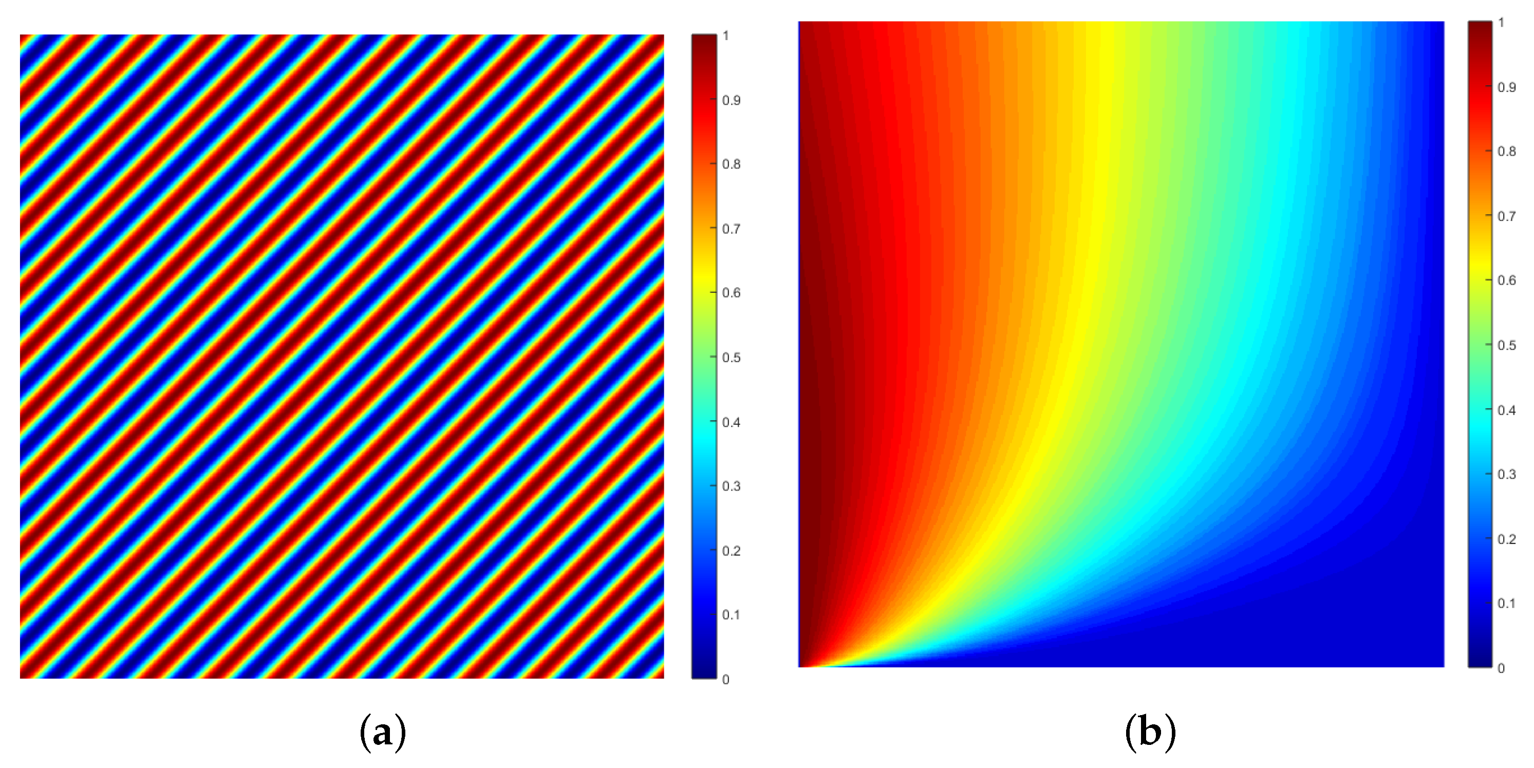
Figure 2 shows example diffraction patterns based on Equations (
38) and (
39) computed using a uniformly sampled grid of 1000 elements for
with
and
. The results have been obtained using the Matlab functions
fft (with
fftshift) and
conv, to compute the Fourier transform and the convolution operations, respectively. In order to enhance the dynamics of the intensity patterns
, the plots are first normalised and plotted on a logarithmic scale given by
.
5.3. Fourier and Fresnel Zone Equivalence
Equations (
38) and (
39) are solutions for the scattering cross-section (the intensity of the scattered wave-field) based on Equation (
34) under the conditions that
and
, respectively. Is there a simple relationship between these two results leading to an equivalence principle? The answer to this question involves using the same equivalence relationship for a Fourier transform that was originally designed to develop a fast Fourier transform algorithm by Leo Bluestein in 1970 [
32]. It is based on re-writing the discrete Fourier transform in terms of a discrete convolution sum. However, this approach can also be applied for the case of continuous functions as shall now be addressed.
The key to developing the equivalence principle is to note that a Fourier transform (for
) can be written in the form
Thus, using the notation for a convolution integral, we can write Equation (
38) in the form
Comparing this result with (
39), where
; then, for the case
, we can construct two equations, namely,
for the scattering cross-section in the Fresnel zone and the Fourier zone, respectively.
In the context of these two equations, and, specifically for the case when , the difference between the diffraction pattern in the Fresnel zone and the Fourier zone becomes the difference between convolving the chirp function with the aperture function and convolving the same chirp function with the conjugate chirped aperture function .
5.4. Quantification of the Born Approximation
Equations (
38) and (
39) are effectively the result of considering different geometric scenarios, both of them being taken under the Born approximation—Condition (
33). It is therefore worth quantifying this approximation within the context of the model considered for the scattering function, namely, an infinitely thin slit.
For this purpose, we consider the condition using a Euclidean norm for
, i.e., an integrable function
for which we can define
Using inequalities (
16), (
17) and (
18), we can write
and Condition (
33) therefore becomes
Given the expression for
provided by Equation (
32), and, using polar coordinates
, then
Thus, defining the root mean square of
as being
the condition for the Born approximation to be valid can be written as
This is the condition for the scattering of a non-relativistic electron or ion beam, quantified by Equation (
26). For the case of a beam of photons quantified by Equation (
24), the difference is that
is replaced by
. The condition for the Born approximation to be valid is then given by
These conditions have been derived for a disc with radius
R, which is a measure of the square root of an area. For an infinitely thin slit of the type illustrated in
Figure 2, the area is negligible, and, in this context, both the conditions (
40) and (
41) are valid. Note, however, that, in the latter case, and, in general, we require that the wavelength
is significantly larger than the physical dimensions of the scatterer, i.e., for a given value of
, we require that
. In other words, for an infinitely thin aperture (or otherwise), the width of the aperture must be small compared to the wavelength in order to generate a diffraction pattern. In the case of Condition (
40),
.
6. The Electromagnetic Shutter Problem
Having reviewed time-independent scattering for under the Born approximation for an infinitely thin aperture, and obtained expressions for the intensity of the diffraction pattern in the plane, we now consider the time-dependent case for and for a scalar EM wave. In this context, the plane considered previously is replaced with an map. The purpose of this is to emphasise the fact that, while the characteristics of the time-independent diffraction of EM and QM fields are essentially the same, the time-dependent shutter problem is markedly different for the two fields.
With reference to
Figure 1, we consider a unit amplitude plane wave that is incident on a shutter, which is opened instantaneously at
. The width of the wave-field is taken to be less than the width of the aperture so there are no diffraction effects. In this case, for
, Equation (
22) becomes
where
, with initial conditions given by
To solve this problem, we consider the time-dependent Green’s function (for
). In this case, the Green’s function is given by the solution to
where the notation
denotes
.
Time dependent problems of this type require application of the Laplace transform. This is because the (one-sided) Laplace transform is a causal transform and therefore provides the facility to implement initial values for the field
and/or its derivative at
. Using Relationship (
11), Equations (
42) and (
43) transform to
where
and
where
respectively.
Pre-Multiplying Equation (
44) by
G and Equation (
45) by
u, subtracting the results and then integrating over
x and
t, we can construct a solution for
given by
for
and
.
The values of
and
at
are un-specified. Moreover, given that they can be taken to be beyond the spatial domain of interest, they are irrelevant, and can therefore be set to zero. This is consistent with the asymptotic condition that
as
. Thus, given the initial condition specified, we can consider the solution
Inverse Laplace transforming, and, noting that
we then obtain the time-dependent solution
given that
.
The time-dependent Green’s function—the solution to Equation (
43)—is given by (for
)
This result can be obtained, by taking the inverse Fourier transform of the time-independent (out-going) Green’s function, which, for
, is given by
Thus, using Relationship (
2), and then applying the convolution theorem,
Given that, for
,
then, from Equation (
46), we have
which describes a wave travelling from left to right (using the quantum mechanical convention [
33] in the positive half space of
Figure 1).
Figure 3a shows a space-time map of the real component of
for
computed for a regular grid consisting of
elements and displayed using the Matlab
jet colour map after normalisation—a map of
. Note that the intensity of the field
in this case is a constant
.
The solution given by Equation (
46) is dependent on the initial condition
. For the case when this condition is non-zero, the equivalent solution is
For example, if the initial wave function in the negative half-space is
then
9. The Quantum Shutter Problem
As discussed in the Introduction, the ‘quantum shutter’ problem leads to the principle of ‘diffraction in time’ which is a fundamental transient phenomenon in quantum mechanics. In this case, we consider a pencil-line beam of non-relativistic particles described by wave-function
, which satisfies the time-dependent and one-dimensional Schrödinger’s equation. For
, and, using natural units
, we are interested in a solution to the equation
subject to an initial condition
.
With references to
Figure 1, the initial condition is taken to describe a unit plane wave that is incident upon the shutter before it is instantaneously opened at
and the particle beam is allowed to pass through. The beam is described by a right-traveling unit amplitude plane wave
which is incident upon a closed shutter placed at
.
The shutter is initially taken to be a perfect absorber so that, in the positive half-space,
. It is then opened instantaneously at
after which the particle beam is free to travel into the positive half-space. The problem is to find the transient behaviour of the particle beam once it has been made ‘free’ to travel in the positive half-space after the shutter has been opened subject to the initial condition
If we consider this problem in regard to the propagation of photons, then the wave function
, is governed by the classical wave equation as discussed in
Section 6. Intuitively, one would considers the photons to propagate into the positive half-space after the shutter is opened so that, for
, this half-space is characterised by a linear wave traveling from left to right as verified in the analysis presented in
Section 6. However, for a beam on (non-relativistic) electrons, the physical behaviour is entirely different. This is a consequence of the nature of the Green’s function, which, given Equation (
14), for
,
, and imaginary time
becomes
which is the Green’s function for Equation (
66),
Following the approach to generating a Green’s function solution given earlier in the paper, the solution for
is given by
illustrating that, like the classical diffusion equation,
as
.
9.1. Solution for the Schrödinger Equation
Compared to a beam of photons, the transient behaviour associated with a beam of electrons, for example (subject to the instantaneous opening of a shutter), is determined by a chirp function. This is a direct consequence of Equation (
66) being characterised by the (imaginary) time derivative operator
compared to Equation (
22)—for
—which is characterised by a second order (real) time derivative operator
. This is also the case for the multi-dimensional Schrödinger equation (for
)
given that, from Equation (
14), the Green’s functions for this case are given by
The solution given by Equation (
68) can be studied analytically using a change of variables to obtain an expression for the probability density given by [
1]
where
and
and
are the Fresnel integrals
However, Equation (
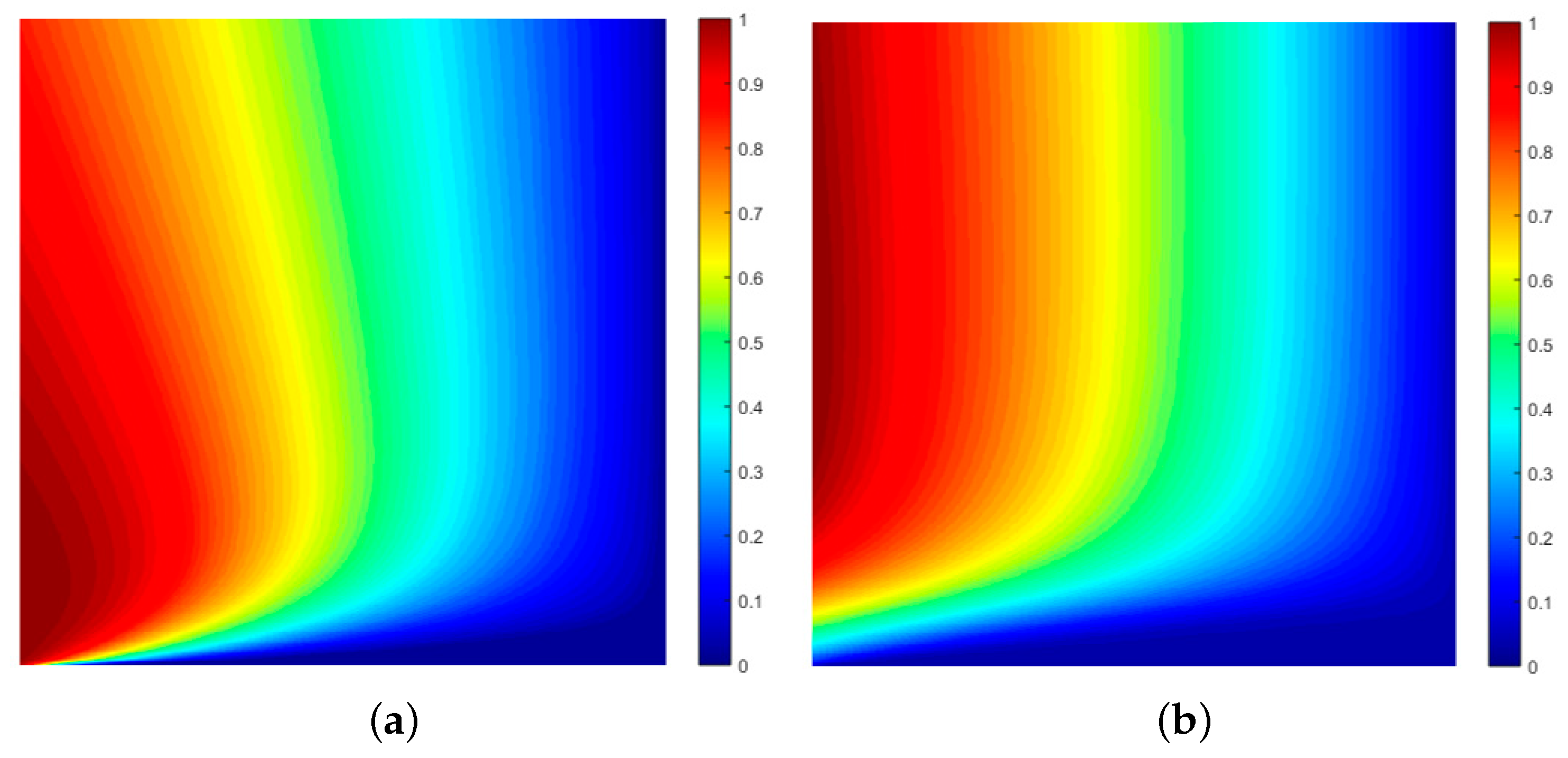
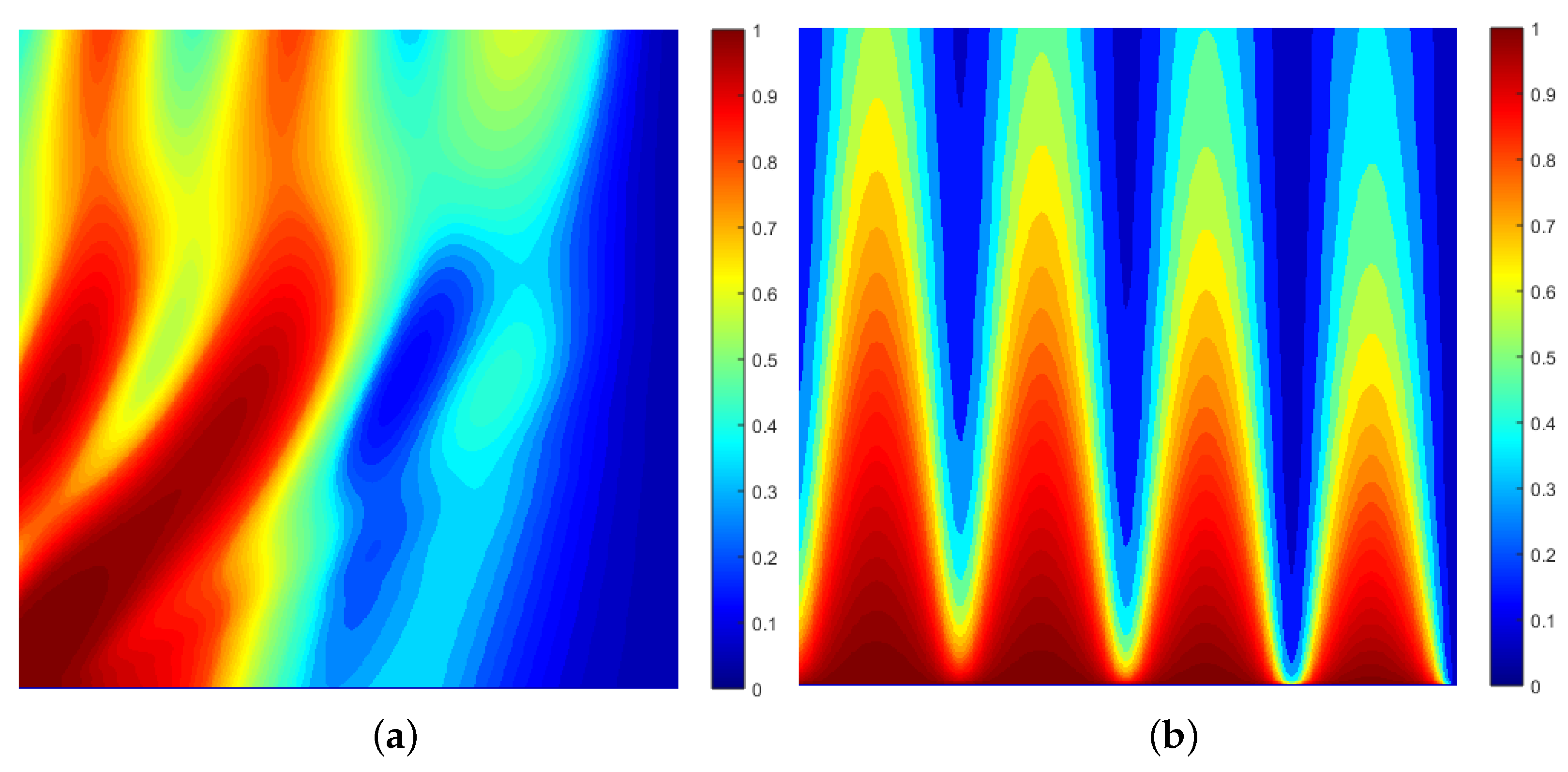
68) can also be computed numerically via application of a convolution sum and the solutions displayed on a space-time map of the type given in
Figure 3. Two examples of this are shown in
Figure 5, which provides time-diffraction maps of the probability function
, where
is given by Equation (
68). In both cases, the function
is computed on a uniformly sampled grid consisting of
elements and displayed using the Matlab
jet colour map after normalisation, i.e., a map of
. The maps have been enhanced using the Matlab histogram equalisation function
histeq. They show examples of the oscillations in time (and space) that decay over time and decrease in frequency, the effect being dependent on the value of the wavenumber
k associated with the initial condition compounded in Equation (
67). As the value of
k increases, the oscillatory behaviour ‘expands’ over the
plane.
The examples given in
Figure 5 illustrates the oscillatory behaviour and decay of the probability density function for non-relativistic electrons. This is of course very different to the optical case (a beam of photons characterised by the classical wave equation as presented in
Section 6) when, by comparison, the intensity function in the positive half-space is a constant, i.e.,
Figure 3a would be a map of the value 1. There is a similarity between the expression for
given by Equation (
68) to the Fresnel zone solution given in Equation (
39). This is why the transient phenomenon associated with the quantum shutter problem is dubbed ‘diffraction in time’ [
1]. It is a quantum effect that requires the application of very low velocity particles, observed over small distances, so that the time interval of an experimental observation is very small, when the Fresnel-type oscillations of the density function in time are prevalent as illustrated in
Figure 5.
9.2. Solution for the Space Fractional Schrödinger Equation
In
Section 8, the fractional diffusion equation was constructed from Equation (
53) on the basis of a delta memory function and a PDF given by
. Suppose we apply the same (phenomenological) principle for constructing the space fractional Schrödinger equation, but for the imaginary memory function
. In this case, because the delta function is imaginary, the field
can no longer be taken to be a density function but a complex wave-type function (on a phenomenological basis). In this context, with
, where
has dimensions of
, and
, we recover the fractional Schrödinger equation (for
)
which is an identical equation to Equation (
60) for imaginary time
and with
. Thus, we can use the solution given by Equation (
65) for the initial condition given by Equation (
67), i.e.,
but where the Green’s function (for
) is now given by
In this case, it is noted that the Green’s function includes an exponential decay which is eliminated as
for all values of
x and
t, conforming to Condition (
63), and/or as
and
.
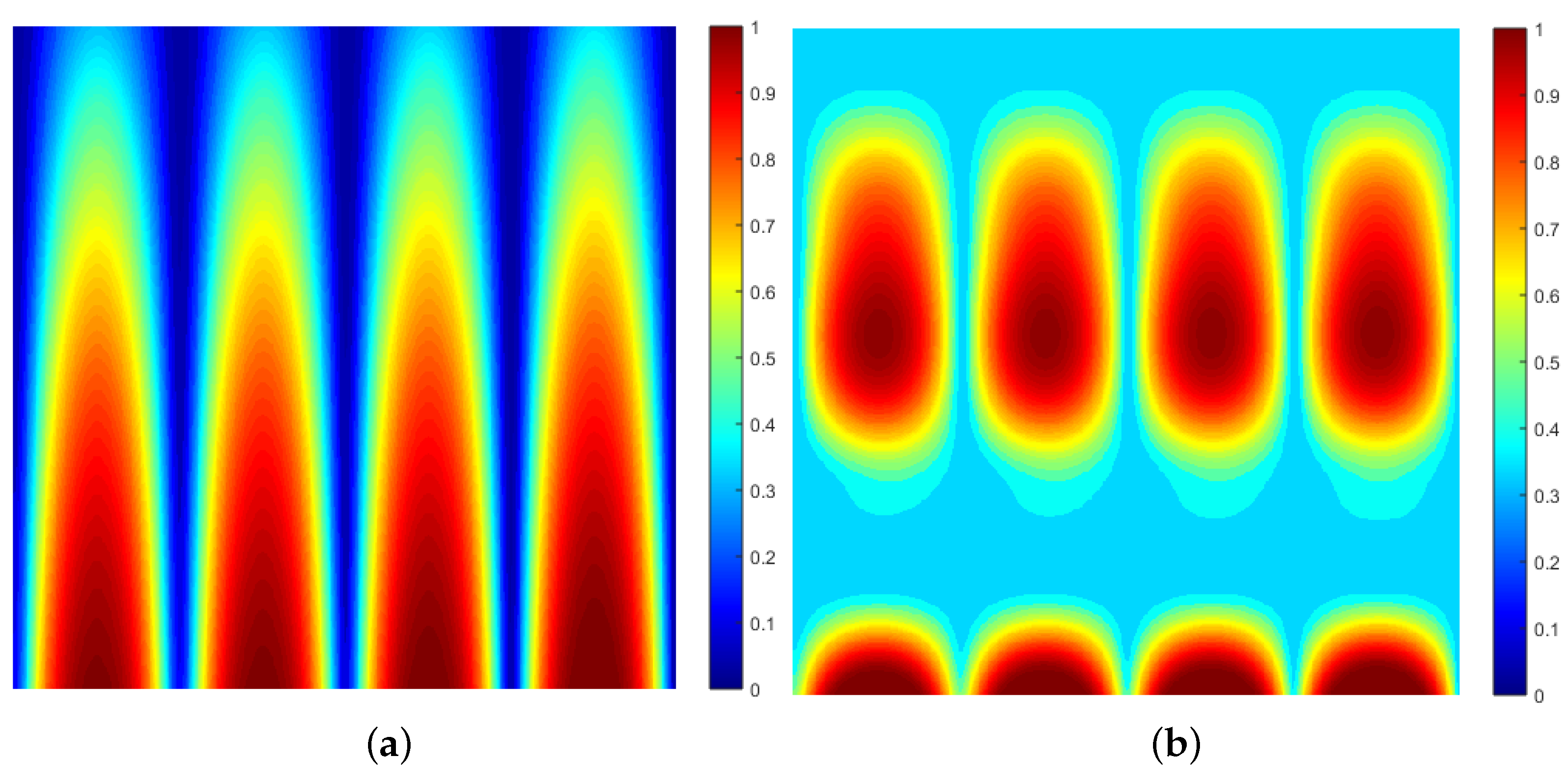
Two examples of this solution are shown in
Figure 6, which provides maps of the probability function
, where
is given by Equation (
70). The function
is computed on a uniformly sample grid consisting of
elements and displayed using the Matlab
jet colormap after normalisation—a map of
. The maps have been enhanced using the Matlab histogram equalisation function
histeq.
These results are illustrative of the fact that, close to the shutter, and, as time increases (after the shutter has been opened), then, for
, and, for
, the probability density forms
n fringes which decay over time. However, as
, the decay over time is eliminated, and, consequently, the density function forms a standing fringe pattern that is constant in time. If such a density function could be generated experimentally, then it could form a periodic grating for the diffraction of an electron beam, for example that is perpendicular to the plane of the grating, for which the diffraction models given in
Section 5.2 become relevant.
9.3. Time Fractional Solutions
Having discussed the space fractional quantum shutter problem in the previous section, we now consider the time fractional case. This is based on using a memory to represent a fractional time derivative given that
. For this range of
, the operator
is an anti-fractional derivative—a fractional integrator. The most basic fractional integrator is the Riemann–Liouville integral which can be defined as
In the context of this definition, and, with respect to Equation (
53) with
, we consider a time fractional diffusion equation given by
where
and it is noted that
However, for
, when the classical diffusion equation should be recovered,
and thus
a result that is incompatible with the expected limit
. This incompatibility is due to the fact that the transform
is strictly only applicable for
. Thus, in order to construct a memory function that is compatible with the expected result when
, we can define it as
noting that
9.3.1. Time Fractional Diffusion
Following the approach detailed in
Section 7.4, we can now construct a solution for density field
given by (for
)
where
Compared to the solution for the space-fractional diffusion equation, the time-fractional case includes a causal convolution in time with the memory function. Furthermore, comparing the fractional indices, it is clear that .
9.3.2. Time Fractional Quantum Shutter
This same principle applies to developing a solution for the time fractional shutter problem. This essentially involves replacing
t for
when the solution given by Equation (
71)—for the wave function
—is given by
where
and
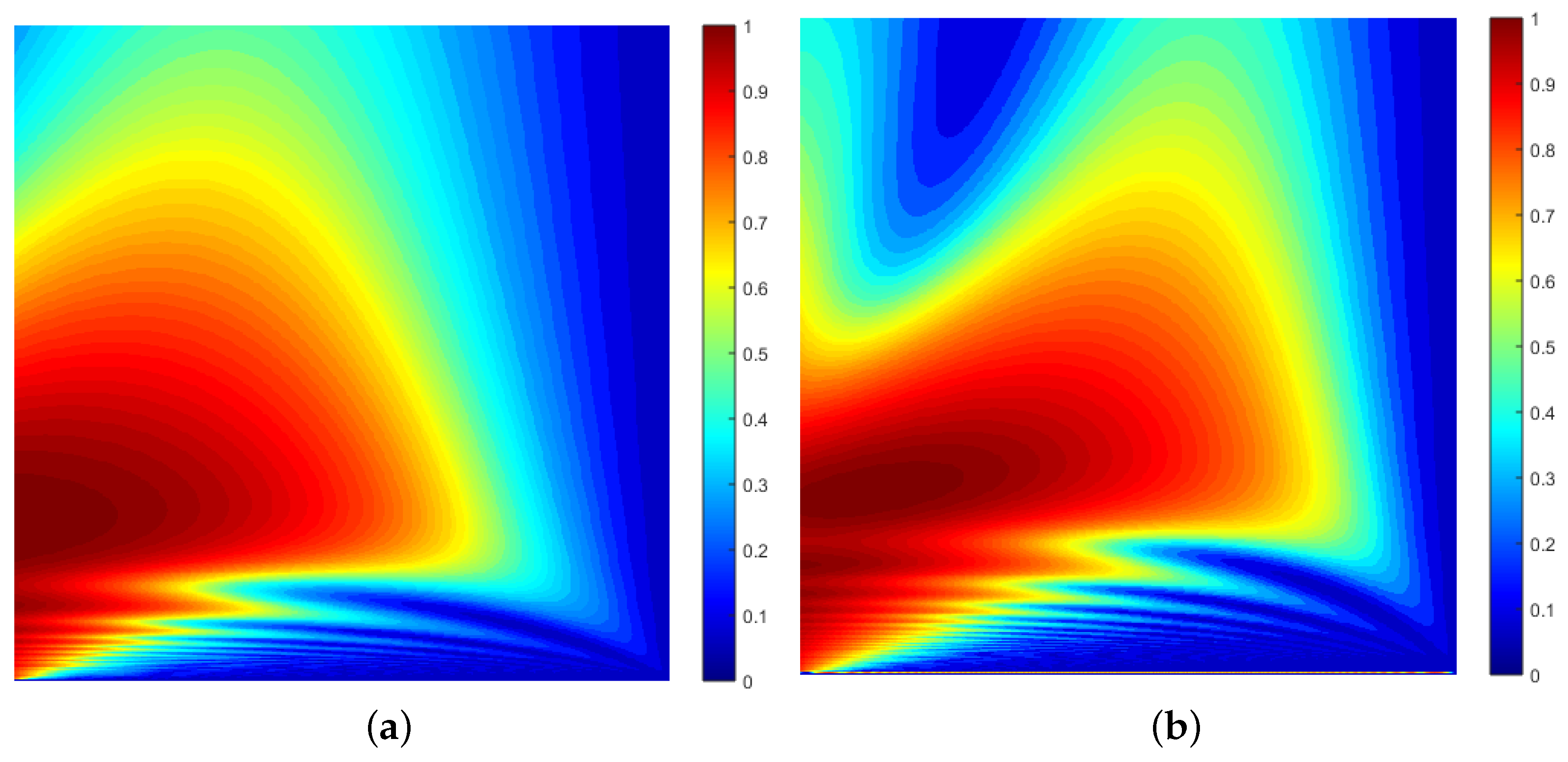
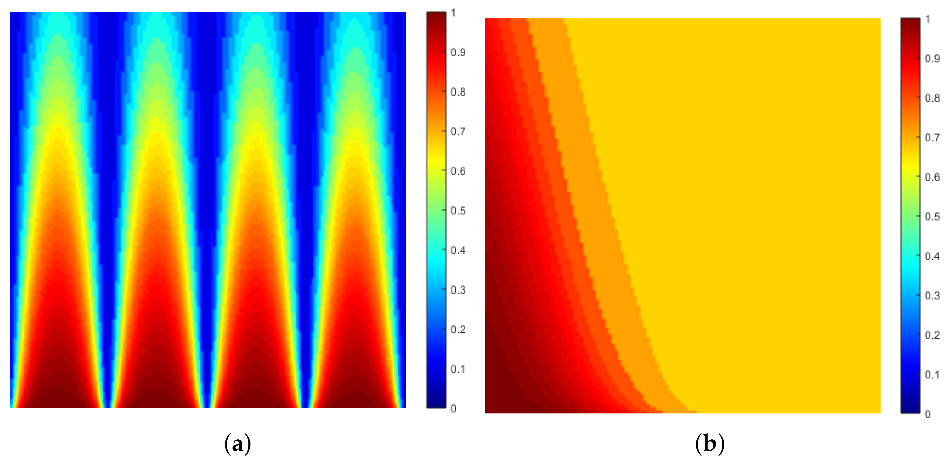
Two examples of the solution given by Equation (
72) are shown in
Figure 7, which provides maps of the probability density function
. As in previous results, the function
is computed on a uniformly sample grid consisting of
elements and displayed using the Matlab
jet colormap after normalisation giving a map of
, the maps having been enhanced using the Matlab histogram equalisation function
histeq.
The results illustrated in
Figure 7 show that oscillations in time are prevalent when
as should be expected, when the solution approaches that of the solution presented in
Section 9.1, compounded in
Figure 5. However, the time oscillations do not reflect that of a Fresnel diffraction pattern and are of a significantly lower frequency for the same initial condition
. On the other hand, as
, the probability density reflects the standing fringe pattern illustrated in
Figure 6, for example, for the space fractional case, but with a greater dissipation in both space and time.
11. Conclusions: Summary and Further Work
Coupled with a review of the more relevant materials, and, coupled with appropriate references, the principal focus of this paper has been to study the quantum shutter problem for fractional quantum fields. In this context, both the space-fractional and time-fractional Schrödinger equations have been considered. Furthermore, the same shutter problem has been considered for a phenomenological equation, which represents the case when the quantum ‘system’ is semi-relativistic.
In all cases, the term ‘shutter problem’ refers to the case when a shutter is opened instantaneously at time , subject to an initial condition . The problem is then to evaluate the probability density of the quantum field in the positive half space for all .
11.1. Summary
The study reported in this paper represents an extension of the shutter problem to the field of fractional quantum dynamics. The paper has attempted to explain the models and solutions thereof in terms of a broader connectivity with classical diffraction phenomena and the classical and fractional diffusion equations. This has been done in order to unify the physical models associated with time-independent and then time-dependent phenomena with regard to the interaction of a field with an aperture which is open over all time or opened instantaneously at , respectively.
In order to contextualise the fractional dynamical models considered, the associated non-fractional models and solutions thereof have been presented. This has been done in order to produce an integrated framework, and to provide reference points to prior art. In both cases, the essential key to developing a solution is to evaluate the Green’s functions for the linear differential operator, fractional or otherwise. Once this function has been evaluated, its convolution with some initial condition provides the basic solution. In this context, the paper has explored solutions to the following:
The time fractional diffusion equation;
The space fractional diffusion equation;
The space fractional Schrödinger equation;
The time fractional Schrödinger equation;
The time fractional Klein–Gordon equation.
Example results have been presented to illustrate the behaviour of the solutions as a function of space and time. This has been done by providing enhanced colour maps of the solutions to illustrate the dynamical behaviour of the probability density. In order to provide an example of the Matlab code used to obtain the result presented,
Appendix C provides the m function used to generate the maps given in
Figure 5. This function is just one of many that have been generated to output the field maps presented throughout this paper. It is provided as a basic exemplar for the sake of interested readers who may wish to repeat the results given and extend them further.
In the case of the time-fractional problems considered, the issue of defining an initial condition for a fractional time derivative has been addressed through the application of a memory function. Here, a fractional time derivative is represented in terms of a first derivative in time, convolved with the memory function. The memory function is chosen so that application of the Laplace transform yields an expression which incorporates the required initial condition for the field at . This provides an explicit indication of the fact that fractional time derivatives are consistent with modelling a memory associative system.
11.2. Future Work
The analysis presented in this paper has focused on one-dimensional models, providing maps to illustrate the one-dimensional dynamical behaviour of the solutions derived. Thus, an obvious extension is to consider the same approach for multi-dimensional models for both space- and time-fractional cases. In this respect, a further, and, more quantitative, analysis is required, based on the methods presented and their extension to multi-dimensional models, subject to a variety of initial conditions. In other words, the results presented are only illustrative examples of a wide range of results that characterise dynamical behaviour based on variations of the fractional exponents and , for the space-fractional and time-fractional derivatives, respectively.
Another area of interest is to compare the multiple scattering solution provided in
Appendix A with the time-fractional diffusion equation for the operator
. In principle, this operator describes the intermediate case when scattering interactions are neither fully diffusive (
) or fully ‘propagative’
. In this context, such an operator can be used to model a scenario where multiple scattering interactions occur for a limited number of scattering sites; where the density of scatterers reduces to 0 as
, yielding a model for propagation in a homogeneous half-space. If all scattering sites are taken to be Coulomb potentials, then the results can then be compared directly with the solution given in
Appendix A, subject to
as discussed in Corollary A2. In this respect, the development of an exact scattering solution for the space fractional Schrödinger equation may be undertaken using a similar approach.
The numerical results presented have been based on the use of a convolution with the corresponding Green’s function, a function that, for both space- and time-fractional models, is based on an approximation in which the field is taken to be observed close to the shutter when
and where
. These conditions have been used so that the Green’s function has a similar form to the Green’s function for the classical diffusion equation. However, there is another approach to developing a numerical evaluation of the fractional quantum fields that can be considered. This is to use the approach presented in
Section 3 and
Section 3.3, given that the Mittag–Leffler function can be computed numerically [
30], coupled with the application of an inverse fast Fourier transform.
For the time fractional Schrödinger equation, written in the form
we can evolve the solution
This solution may then be investigated by computing the Mittag–Leffler function numerically, applying an inverse fast Fourier transform to the result, and convolving the output with the initial condition.
For the time fractional Klein–Gordon equation considered in
Section 10.2, if we consider the equation (where
)
subject to the initial conditions
and
, then a solution based on an application of the Mittag–Leffler function can thus be constructed:
A numerical evaluation of the fractional quantum field can then be investigated by computing the functions
and
numerically [
30], applying an inverse fast Fourier transform and convolving the results with the initial condition(s).
Finally, an investigation should be undertaken into the time-fractional Dirac equation for the quantum shutter problem, following the approach taken in [
13], for example.


