1. Introduction
In today’s engineering practice, analyses of very complex systems are frequently studied based on various finite element methods (FEM) and computational fluid dynamics (CFD) tools. The sophistication of these simulation packages and their direct connections with solid modeling and engineering graphics tools have inadvertently left false impressions among design engineers that the fundamentals of solid and fluid mechanics are no longer needed. In fact, some of the design engineers tend to utilize simulation packages right at the beginning stage of the design process at which the entire system and its geometries and configurations are still not finalized. As a consequence, the intricate design details and specifics which are not finalized will be entangled with the complication of meshing and multi-scale issues for both FEM and CFD analyses. In a way, this is very similar to applying high resolution or magnification lenses during preliminary search within a fairly large area, which is obviously very ineffective, inefficient, and wasteful with respect to both time and financial resources.
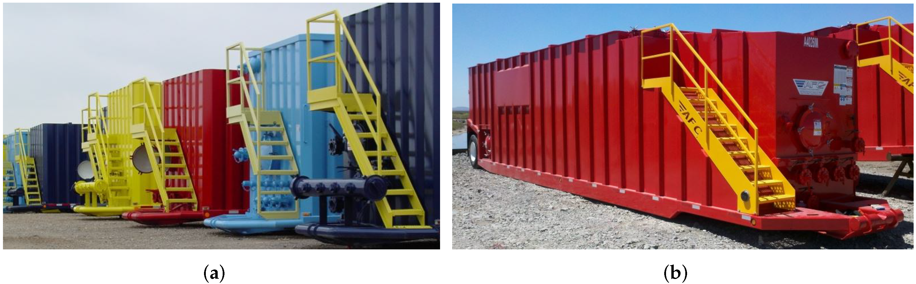
Wichita Tank Manufacturing LTD presented the McCoy School of Engineering with a design concern with respect to their
holding tanks for hydraulic fracturing, as shown in
Figure 1. In the United States of America, most fluid barrel apart from oil barrel has the following conversion ratio, namely,
is equivalent to
or
Initially, these tanks were designed to hold up to 15,750 gallons of water. While it is empty, the tank will be transported through highway systems to and from different locations. The problem is to determine whether or not it is safe to hold the same volume of heavy liquid such as mud. To be more precise, whether the current dimensions and design could withstand the pressure of mud with typical specific gravity up to
with
sand and
water by mass or weight. The typical density for fresh water, denoted as
is
or
, or
. The typical density for sand, denoted as
is
or
. Notice that the reciprocal of the density is the so-called specific volume
v. For mud, namely, sand and water mixture, denote the mass ratio of the sand as
x, a similar concept to the quality factor of the steam representing the mass ratio of the vapor within the steam, the specific volume for the mud can be expressed as
where
and
stand for the specific volume of the sand and water, respectively.
Figure 1 shows the typical holding tanks with lateral reinforcement and auxiliary systems. Since a large number of such holding tanks will be manufactured, the saving for structural materials and manufacturing costs will be significant and should justify the in-depth analysis of structural designs. Unlike the permanent foundations for the holding tank which have been studied in Ref. [
1], the holding tank of interest in this study is a stand alone structure. Moreover, seismic impacts and ground motions on storage tanks have been presented in Refs. [
2,
3]. In this paper, the static or quasi-static stress analysis is the focus for holding tanks under the extreme hydrostatic loading. The complexity comes from the extreme geometrical aspect ratios of three-dimensional plates and stiffeners. Currently, all these tanks are made of low carbon steels which can be easily welded with channel beams as stiffeners. Buckling analysis and homogenous properties of composites for lighter and more adaptable designs of deployable structures have been discussed and presented in Refs. [
4,
5,
6,
7]. Furthermore, contact stress and surface conditions are also ignored in this study. For studies of mechanical behaviors of grinding and cutting as well as brakes and clutches, silicon dioxide ceramic matrix composite and fiber reinforcements become key features in multi-scale and multi-physics material modeling [
7,
8].
Moreover, in this paper, the material failures due to corrosion and fatigue as elaborated in comparison with structural failures in Ref. [
9] will be considered. To be more specific, typical simplification processes in structural mechanics are employed whereas stiffeners and plates are modeled as I-beams whose geometric center is at a distance away from the plate surface as shown in
Figure 2. In one-dimensional beam model, the plate is considered as the top flange in combination with the channel beam or the stiffener as the web and bottom flange; likewise, in two-dimensional plate and beam model, the entire plate is modelled with the stiffener rigidly linked without the plate as its top flange as depicted in
Figure 2.
Through the hierarchical study presented in this paper, the current holding tank design with a height of , a width of , and a length of along with ASTM A36 stiffeners spaced approximately apart at centers made with a quarter inch thick ASTM A36 steel is confirmed to withstand the heavy liquid with the density of . The detailed stress analyses also shed some light on the subject about the manufacturing process as well as the validation and verification of the structural designs. In the past, wide steel plates are employed with the gap between the corrugations as . Due to a price difference of sheet metals, wide sheets will be employed in the future. Through the hierarchical modeling presented in this paper, engineers will be able to determine whether or not it is possible to enlarge the gap to 16 or while maintaining the same design limit of the liquid pressure with the threshold density of , or . Finally, with such a set of comprehensive structural analyses, more design details and improvements will be proposed with respect to stiffeners and smooth transitions for local structures as well as horizontal and vertical reinforcements.
2. Beam, Column, and Plate Models
In structural designs for the holding tank, the hydrostatic pressure occurs in a non-uniform fashion which is dependent on the depth of the liquid as illustrated in
Figure 3. The reinforcements of the holding tank wall are very similar to ship hull and airplane structures. Although full-fledged three-dimensional solid models can be implemented with a finite resolution, considering the extreme geometrical aspect ratios as presented in this paper, it is always desirable to have approximations with the consideration of these non-uniform pressures distributions which can yield empirical formulas with physical insights as illustrated in Ref. [
10]. Before the elaboration of computational and analytical approaches for the complex structural systems as illustrated in
Figure 1,
Figure 3, and
Figure 4, one and two-dimensional analyses as well as corresponding finite element models have been employed and compared. In this slightly simpler, yet also challenging example as shown in
Figure 4, which can be viewed as a reinforced steel plate commonly used as a sluice or slide gate with both ends completed fixed with the dam or the wall, the stiffener is made of a channel beam with a width of
, a depth of
, and a uniform thickness of
. The overall height of the sluice is
and the total width of the sluice is
. From the smallest structural component with a thickness of merely
to the overall dimensions around a few hundred inches, this seemly simple structural example is also a complex structure with extreme geometrical aspect ratios. In this study, the same hierarchical modeling techniques will be employed. In addition, both plate and beam model and full-fledged three-dimensional solid model will be compared with analytical approximations.
In the so-called zeroth order approximation as illustrated in
Figure 2, the middle portion of the plate centered around the stiffener with a width
b as a half of the total width, namely,
, is taken as the approximation of the complex structural system. Thus, the largest hydrostatic pressure can be expressed as
, where
h stands for the largest depth of the water,
is the water density and
g is the gravitational constant. In some texts, the hydrostatic pressure is also denoted as
, where
is the so-called specific weight. Again, as shown in
Figure 2, in the zeroth approximation, the plate with a width of
is attached to the stiffener with the dimension
Thus, a beam is essentially made with a cross-sectional area made of one
area
, two
areas
, and one
area
. If the origin is placed at the top center of the stiffener as illustrated in
Figure 2, the center of the area of the cross section
can be easily calculated, given the local geometrical center and the local second moment of area for these three regions as
,
, and
, respectively,
Furthermore, given the local second moment of area about
y axis passing through its geometrical center for these three regions as
,
, and
, respectively, the total second moment of area for the entire cross section can be written as
which by converting the cross section into an square yields an equivalent side
a as
Assume a tip concentrated load
P, at the depth
z, with the tapered pressure distribution from 0 to
, the bending moment
can be expressed as
where
b is the width of the total hydrostatic pressure acting on the sluice or the gate.
Therefore, the internal strain energy can be summarized as
and with the Castigliano’s Theorems the tip displacement
can be expressed
Therefore, based on Equation (
6), substituting the typical Young’s modulus for low carbon steel
E as 30,000 ksi, the density of the water
as
, the gravitational acceleration
g as
, and the equivalent square cross section second moment of area as
with the equivalent edge size
a as
the zeroth order approximation of this complex structure example as illustrated in
Figure 4, is evaluated as
In the so-called first-order approximation, the effect of the plate can also be substituted with an equivalent distributed stiffness
k as shown in
Figure 2. Consider a slice of the plane strain plate with a unit width and the same thickness
t which are fixed on both ends, a displacement (in
x direction) distribution with the peak value
in the middle can be expressed as
where the length
L of this slice of the plate spans the full width of the sluice or the slide gate which is
.
The total strain energy for the unit width can be expressed as
where
D is the so-called bending rigidity for the plane strain plate with a thickness
t and denoted as
with the Young’s modulus
E.
The equivalent strain energy for the unit width can be depicted as
where with the Poisson’s ratio
as
the distributed stiffness
k can be derived as
Notice that in this first-order approximation, the entire plate is taken into consideration as the distributed stiffness therefore, the beam cross section only consists of the stiffener with two area
and one area
as shown in
Figure 2 and
Figure 4. Thus, given the local geometrical center and the local second moment of area for the region
and
as
and
, respectively, the geometrical center of the entire cross section is expressed as
Furthermore, given the local second moment of area about
y axis passing through its geometrical center for these two regions as
and
, respectively, the total second moment of area for the entire cross section can be written as
which by converting the cross section into an square with an equivalent side
a as
In the first-order approximation with the distributed stiffness in lieu of the effects of the plate, in order to calculated the tip displacement, a pseudo tip force
P as illustrated in
Figure 2 is introduced. Thus the bending moment at the depth
z, with
, can be expressed as
along with the following, assuming small displacement and deformation, with
,
Employ the boundary condition at the bottom with
, namely,
and
, the two coefficients
and
can be derived as
By introducing the elastic foundation or distributed stiffness
k, the governing equation for the beam can be expressed as
where the distributed load is denoted as
as depicted in
Figure 2.
The homogenous part of the governing Equation (
17) yields the characteristic values
, with
, and 3 and
. In practice, by utilizing the Euler form
, define
, the characteristic solutions for the corresponding homogenous solution can be expressed as
Naturally, using the Wronskian technique as depicted in Ref. [
11], the analytical solutions for general distributed load
can be established. However, for simplicity, the Galerkin method can also be employed, and the approximation can be established as
which yields the tip displacement
B along with
,
,
, and
Notice that three out of four boundary conditions of the cantilever beam are satisfied which suggests that a fairly accurate numerical solution of the tip displacement
B. Thus, instead of satisfying the governing equation, the following weak form holds
or rather with the implementation of boundary conditions,
with the full width
b as
in this case.
Utilizing the following definite integrals
the first-order approximation of the tip displacement
B is derived as
As an extreme case by ignoring the distributed stiffness
k, the tip displacement
B can be expressed
which is consistent with the zero-order approximation established in Equation (
6).
Moreover, the strain energy
U can be expressed as
in which the first term represents the bending strain energy and the second term stands for the strain energy in the distributed stiffness.
Introducing a scaling factor
to gauge the influence of the plate in the form of the distributed stiffness with respect to that of the stiffener,
Finally, the first-order approximation of the tip displacement
can be expressed as
with the width
b as
instead of
for the zero-order approximation.
It is clear that the first-order approximation is much more accurate than the zero-order approximation. The comparison between the two approaches has also established a relative important of the plate in the who structural system. In fact, the plate contributes an overwhelming portion of the stiffness in comparison of that of the stiffener expressed in Equation (
26), namely, nearly 70 to 1 ratio. To validate these approximations, two finite element modeling strategies are adopted, namely, a two-dimensional plate model rigidly linked to stiffeners simplified as beams with the same displacements and rotations via the so-called master node and slave node options in ADINA; and a full-fledged three-dimensional finite element model implemented in ADINA.
For the two-dimensional plate and beam ADINA model, with
nodes,
plate elements, and 40 Hermitian beam elements, as illustrated in
Figure 5, the plate location is placed on the mid-span and consider the neutral axis of the stiffener passing through the center of the geometry without the plate, namely
from the outer edge of the stiffener, the beam linked to the two-dimensional plate through the constraints of both the displacement and the rotation with slave and master nodes is situated at a distance
away from the plate which is situated at its own plane. Based on this two-dimensional plate and beam finite element model in ADINA as shown in
Figure 5, the mid span displacement is calculated as
.
Instead of co-dimension one plates and co-dimension two beams finite element models as shown in
Figure 5,
Figure 6 on the other hand depicts a full-fledged three-dimensional solid ADINA model with 177,192 nodes and 14,720 3D solid elements. In this three-dimensional model, a significant amount of nodes are required even with a fairly coarse structural mesh with one element layer over the thickness direction due to the excessive geometrical aspect ratios of this complex structure. As shown in
Figure 6, the mid node displacement 33.0673 in is comparable to the displacement
predicted by the two-dimensional plate and beam ADINA model as shown in
Figure 5. In comparison with the relatively stiffer two-dimensional plate and beam ADINA model, the full-fledge three-dimensional ADINA model is more flexible and yields a slightly larger displacement. Furthermore, the first-order approximation result as expressed in Equation (
27) is also comparable to those from three-dimensional finite element models. It is important to notice that low-dimensional approximation models do over simplify the three-dimensional structure and yield larger mid span deflections. Nevertheless, the physical insights presented in expressions (
6) and (
27) are extremely valuable with respect to key geometrical dimensions and design variations.
3. Low-Dimensional System Validation
In the previous section, the accuracy and validity of the low-dimensional approximations are addressed in comparison with analytical results. In the process of establishing the zero-order and first-order approximations, the hierarchical modeling procedures for the complex structure similar to that of holding tanks yet very much simplified also include two-dimensional plate and beam models. In particular, an equivalent two-dimensional beam-column structural system as shown in
Figure 2 and
Figure 3 must first be derived. A portion of the plate is attached as the top flange of an equivalent beam with the stiffener as its web and bottom flange. Moreover, the width of the plate is normally equal to the space between the stiffeners, denoted in this paper as
b. In this section, we are to further verify and validate the analytical approaches with the computational simulation for a set of more idealized two-dimensional structure models. Using the symmetry, a simplified beam-column is obtained as shown in
Figure 7, in which
H is used to denote the height of the tank and
W stands for the cross-sectional width.
As illustrated in
Figure 7, if the mid section of the equivalent beam across the equivalent columns is cut open, the internal forces, namely, shear force
and tension force
along with the bending moment
must be introduced. Due to the symmetry, it is clear that the shear force
must be zero. In addition, the rotation and the horizontal displacement at the mid section must also be zero. In order to derive the internal moment
and the tension force
, the energy principle, often called the first Castigliano’s Theorem must also be utilized [
12,
13]. Assuming the internal strain energy for the left half of the beam-column system as
U, and using the symmetry, the following can be established
For the plate stripe assigned to the stiffener, the distributed line load at the vertical location marked by the coordinate
x can be expressed as
, assuming the liquid density
is
, and the side-wall corrugated pattern repeats on
intervals, i.e.,
. Of course, this is the first-order approximation necessary for preliminary design. The width of the side-wall plate will carry the liquid pressure and consequently the equivalent beam-column for the stiffener will be subjected to a line load with a linear distribution also illustrated in
Figure 3 and
Figure 7. For the cut section as illustrated in
Figure 7, with the distributed load
for
, the bending moment can be expressed as
Consequently, the analytical expression of the internal strain energy for the left half of the beam-column system is expressed as
where
y represents the position in the horizontal direction,
x is the vertical coordinate,
I stands for the bending rigidity of the equivalent stiffener, and
E is the Young’s modulus.
For simplicity, in this comparison of analytical solutions with computational results, geometrical constraint
holds. Moreover, ignore the shear strain energy in Equation (
30) and employ the first Castigliano’s Theorem, Equation (
28) can be rewritten and be expressed as
Assume the structural dimension
H is much larger than the radius of gyration of the cross sectional area
A, namely,
, or
, the contribution from the axial deformation can be ignored and Equation (
31) can be rewritten as,
Substitute Equation (
28) into Equation (
31), the following system equation is derived
where the state variables are
and the right hand side vector
and the coefficient matrix is depicted as
Finally, the following solutions for the internal tension and the bending moment can be established at the mid span
Furthermore, the same simplified two-dimensional beam-column system model is introduced with an addition of a virtual vertical load
at the mid span or rather the right side the same location where both the bending moment
and the tension
are placed. Ignore the axial tension strain energy and the shear force strain energy, the total strain energy can be expressed as
and from the first Castigliano’s Theorem, employ Equation (
35) for
and
, the mid span vertical deflection in the same direction as the virtual force
can be calculated as
Before the actual dimensions for this holding tank structural system are implemented, low-dimensional approximations with the same approaches must first be validated with the two-dimensional ADINA simulation as illustrated in
Figure 7. In this simulation, the dimension
H is
with a
cross section with
and the Young’s modulus
E as 30,000 ksi. Therefore, the second moment of the cross sectional area
I can be calculated as
Using the analytical result of the deflection as expressed in Equation (
37), the mid span deflection is calculated as
The mid span deflection predicted in the two-dimensional ADINA model with 60 iso-beam elements and 121 nodes, as shown in
Figure 8, is
which is nearly the same as the analytical solution. Moreover, the mid span tension and bending moment predicted in the same ADINA simulation are
and 10,238 lbf · in, respectively, which again are nearly the same as the theoretical results.
With this confirmation and validation, the simulation is expanded to include more specific design details. For example, the design recommendation with the guidance of the two-dimensional finite element models yields a typical cross section of holding tanks as depicted in
Figure 9, in which a simple curve around the corner is reinforced by relevant stiffeners. This simple design modification will certainly alleviate the stress concentration, yet this simple curve will render the elegant analytical procedure untenable. Therefore, full-fledged finite element simulations are becoming a necessity. In fact, contrary to the analytical procedure, such a design modification can be simply handled with similar two-dimensional finite element models as shown in
Figure 10. Note that the overall structural system becomes more flexible with the corner modification which can be simply rectified with straight side walls directly welded to the tank bottom as shown in
Figure 11. Finally, these two sets of structural examples and available analytical solutions have validated and verified the same hierarchical modeling procedures to be implemented along with computational tools such as ADINA and Solidworks for the systematic study of these hold tanks with extreme geometrical aspect ratios.
All stiffeners in holding tanks are made of
ASTM A36 steel channel construction as illustrated in
Figure 12 along with the density of
and the Young’s modulus of 30,000 ksi. The geometrical center is in the mid section of the equivalent stiffener with a distance
away from the edge of the channel stiffener. Assuming the spacing between the stiffeners is
, namely,
, geometric center
is calculated as
and
. If the spacing is increased, for instance,
, the geometrical properties are calculated as
and
.
Note that for metals, the estimated elastic stress limit is about of the Young’s Modulus, roughly, 30,000 ksi, i.e., 60 ksi. The documented yield strength is around . This means under no circumstance, in a proper engineering design, operational stress should approach 30 ksi with a reasonable safety factor. In fact, all these calculations are based on static force and moment equilibrium. If consider the dynamic loading and safety factors, the actual operation stress should be much lower than this level.
Using Equation (
36), the following distribution of the bending moment is established as
with the dummy variable
.
As depicted in
Figure 13 with the solid line, the maximum bending moment is triggered at the bottom of the tank, namely, at
or
,
can be established. In addition, the local minimum also occurs at
or
with
For water density
, if the spacing
b between the stiffeners is
, with
ASTM A36 steel channel construction, the geometrical effects
and
yield
. The corresponding local minimum
. For mud with
, the same maximum stress yields
along with the local minimum
. If the spacing is increased to
with
and
,
and
can be established for water as well as
and
for mud. The trend is very clear that, in general, if the spacing between the stiffener increases, the maximum stress due to bending increases as well, in addition, the deeper the holding tank, the higher the maximum stress due to bending. Considering the stress concentration factor, thermal stress, residual stress due to welding, these current designs of holding tanks are very close to the material design limit.
With the confirmations of both analytical and computational hierarchical procedures, it is now possible to add design details to the full-fledged finite element models. We will adopt both Solidworks and ADINA for the handling of the full-fledged three-dimensional complex structures. In ADINA model, instead of using the three-dimensional solid modeling, co-dimension one plate models are employed along with co-dimension two beam models. Furthermore, to avoid the extreme geometrical aspect ratios, stiffeners can modeled as co-dimension two beams positioned at its own geometric center. For the stiffeners constructed with
ASTM A36 steel channel, without the attachment of the plate, the second moment of area is
with the center of geometry from the baseline
is
Thus, in ADINA simulation, the equivalent beam with a square cross section has the side dimension of
Notice that rigid links are introduced to connect the beams which represent the stiffeners and are positioned at a distance equivalent to the distance from the stiffener baseline to the center of the geometry, i.e.,
Of course, the hydrostatic pressure is based on the mud density
is
and the tank depth
H is
. Moreover, in this quasi-static problem, the static pressure due to the mud specific weight will be assigned over thirty time steps in order to avoid the complication due to excessive deformations. The average Young’s modulus
E for low carbon steels is 30,000 ksi, the Poisson’s ratio
is
. In this full-fledged three-dimensional ADINA model, 10,642 nodes and 19,520 plate elements coupled with 840 3D iso-beams are employed to represent the three-dimensional solid plate and stiffeners. As illustrated in
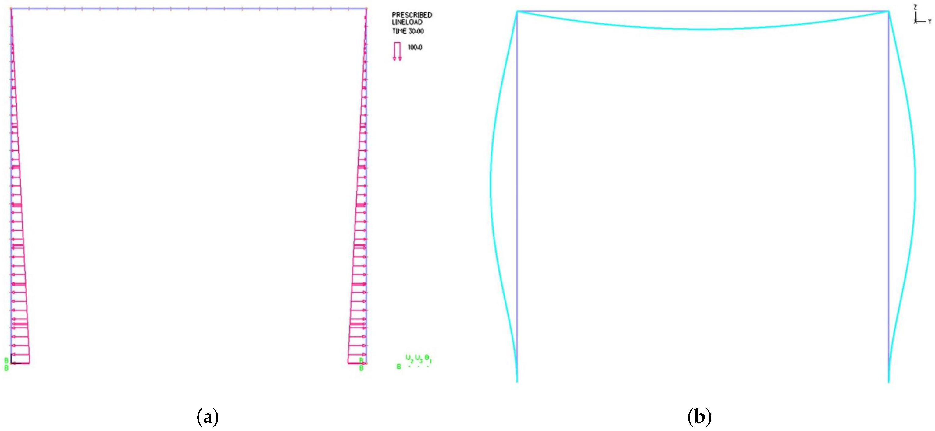
Figure 14 and
Figure 15, the peak deformation is around
, a fairly visible deformation which indicates the design is approaching the material limit as suggested in the simplified analytical models presented earlier in this paper.
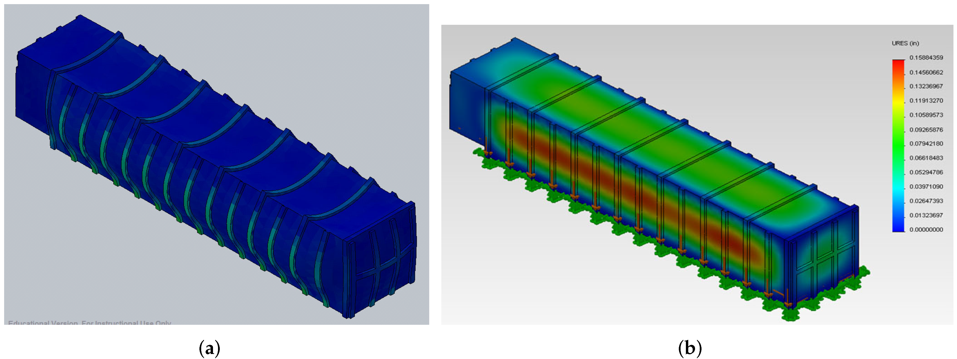
As shown in the three-dimensional model using a software package called Solidworks, it seems that individual stiffeners can be fully expressed as the three-dimensional solid as shown in
Figure 2,
Figure 4, and
Figure 12. Nevertheless, it is very difficult to provide an adequate mesh resolution for stiffeners made of
ASTM A36 steel. Therefore, following the discussions in the previous sections, the stiffeners are simplified by beams with equivalent bending rigidity and rigidly linked to the plate. In
Figure 14 and
Figure 15, co-dimension one plate model stiffened by co-dimension two beam model is represented by finite elements in ADINA. Moreover, in the full-fledged three-dimensional Solidworks model as shown in
Figure 16, additional reinforcements are introduced at the end of the tank structure in comparison with the ADINA model as shown in
Figure 15. It is clear that the finite element Solidworks model using three-dimensional solid elements provides a close yet slightly lower displacement result in comparison with the idealized three-dimensional plate and beam ADINA model. For this stand alone structure, similar fixed boundary conditions as shown in
Figure 17 are introduced on the bottom of both Solidworks and ADINA models. Moreover, also shown in
Figure 15 and
Figure 17 the rigid constraints are utilized to link stiffeners represented by the beams elements with the plate for the three-dimensional ADINA model. With these established models and their respective verifications, engineers can now comfortably engage in necessary design modifications which will further optimize the structural design with the consideration of specific manufacturing requirements and constraints.


