Article

Determination of Detection Probability and Localization Accuracy for a Guided Wave-Based Structural Health Monitoring System on a Composite Structure

1
Mechatronics and Mechanical Engineering Department, Bochum University of Applied Sciences, 44801 Bochum, Germany
2
Civil Engineering Department, Ruhr University Bochum, 44801 Bochum, Germany
*
Author to whom correspondence should be addressed.
Appl. Mech. 2021, 2(4), 996-1008; https://doi.org/10.3390/applmech2040058
Submission received: 20 October 2021 / Revised: 23 November 2021 / Accepted: 27 November 2021 / Published: 2 December 2021
(This article belongs to the Special Issue Damage Sensing in Composites for Structural Health Monitoring)

Abstract

:
The capabilities of detection and localization of damage in a structure, using a guided wave-based structural health monitoring (GWSHM) system, depend on the damage location and the chosen sensor array setup. This paper presents a novel approach to assess the reliability of an SHM system enabling to quantify localization accuracy. A two-step technique is developed to combine multiple paths to generate one probability of detection (POD) curve that provides information regarding the detection capability of an SHM system at a defined damage position. Moreover, a new method is presented to analyze localization accuracy. Established probability-based diagnostic imaging using a signal correlation algorithm is used to determine the damage location. The resultant output of the localization accuracy analysis is the smallest damage size at which a defined accuracy level can be reached at a determined location. The proposed methods for determination of detection probability and localization accuracy are applied to a plate-like CFRP structure with an omega stringer with artificial damage of different sizes at different locations. The results show that the location of the damage influences the sensitivity of detection and localization accuracy for the used detection and localization methods. Localization accuracy is enhanced as it becomes closer to the array’s center, but its detection sensitivity deteriorates.

1. Introduction

SHM systems make a promising technique for monitoring and evaluating the integrity of many industrial structures, such as pipelines, aircrafts, nuclear power plants, and civil structures [1]. SHM systems can be briefly described at four levels: detection of the damage, localization, characterization, and prognostics [2]. Many GWSHM systems compare the current measurements with a baseline response that is considered pristine or damage free by calculating damage index (DI) to determine the current state of the structure [3,4].
The aircraft industry could benefit significantly from using GWSHM systems for damage detection and localization for many reasons: increased safety due to continuous monitoring [5], accessibility to areas difficult to reach for inspection as the sensors are already embedded in the structure, reduced maintenance as it will be scheduled only when required [6], and improved design of aircraft since the critical area will automatically be monitored. Composite structures used in aircraft must continue in flight-safe conditions even with stronger impacts [7]. These substantial impacts cause visible and invisible damage.
Over the last decades, the reliability assessment of non-destructive testing (NDT) has provided information regarding damage detection capability at certain confidence bounds. The methods used for assessing the reliability of an SHM system originated from the guidelines for conventional non-destructive inspection techniques. The POD curve, as a statistical reliability assessment technique, is a cumulative distribution curve generated from an extensive data set obtained at different damage sizes. A generated POD curve provides information regarding the smallest damage size that can be reliably detected or the biggest damage size that may be missed [8]. The basic POD concept is documented in Section 2.3. More details can be found in [9,10,11]. Different methods are applied to assess the detectability of damage: the hit/miss method and flaw size method vs. response ( a ^ vs. a). The hit/miss method produces a binary statement or qualitative information about the presence or absence of damage. In contrast, the ( a ^ vs. a) method provides some quantitative measures.
There are some differences between NDT and SHM systems that change the interpretation of POD curves [12]. Ultrasonic wave testing as an NDT method is based on handheld movable sensor arrays, whereas guided wave monitoring as an SHM method is based on permanently installed transducers with fixed sensor positions. Despite the help of artificial intelligence, data analysis in NDT requires well-trained NDT personnel, while SHM system developers have the firm intention to enable automated inspection and feature extraction. Over the last decades, the community’s primary focus has been developing the SHM system, while few articles focused on the reliability assessment of SHM systems. References [13,14,15,16,17] show first adaptation of POD analysis to SHM systems. Most of these approaches concentrate on hot spot monitoring with guided waves, which eliminates the location dependency. While focusing on one hot spot, [13] analyses the variance of DI and its reasons using simulation and experiment. In [18], the general feasibility of using simulated data for location dependence of POD analysis is shown. In [15], the location dependency is treated as an environmental parameter and the analysis is focused on simulation data. In [14], the specific influence of various parameters is analyzed in a multi-parameter approach.
There has been an increasing interest in visualizing and localizing the damage using a 2D or 3D image [3]. One algorithm that does not depend on guided wave velocities for damage localization is probability-based diagnostic imaging (PDI). The planar area of an inspected structure is first meshed and projected to an image, each pixel corresponding to a spatial point of the structure. The field value of the pixel is calculated using DI, which indicates the probability of the presence of damage at a specific point of the structure. Alternative localization methods are time-of-flight (ToF), time reversal, migration technique, and phased-array beamforming.
Enabling an intuitive visualization, the interest in PDI techniques is high. Tanaka et al. [19] used the statistical window energy arrived method to improve the localization accuracy and sizing of the interlaminar damage and compared it with the classical delay and sum algorithm. Zhao et al. [20] developed a PDI approach, in conjunction with the use of an active sensor network in a pulse-echo configuration to identify the orientation and location of damage such as a notch and crack in an aluminum plate. Liu et al. [21] improved the ability of damage localization with higher precision and lower error on a CFRP composite panel with four T-shaped stiffeners and compared between a developed PDI approach and a developed weight compensated-based damage PDI algorithm. Liu et al. [22] developed a PDI algorithm that localizes the damage within an aircraft pallet. Liu et al. [23] developed an improved PDI algorithm to localize artificial and impact damage on a stiffed composite panel.
Nevertheless, all these references mainly use exemplary damages, locations, and data to quantify the localization error as distance between the center of the actual damage position and the estimated one, while not giving a statistically based analysis on localization accuracy. In [21,22], analysis is performed only for one damage size at different damage positions, and for these positions, values for localization error are given. In [21], an average over all damage positions to quantify the localization accuracy was also calculated. In [23], the localization error varies between (25–50) mm for the impact damage and (4–25) mm for the artificial damage. They emphasize on the development of novel localization techniques, while statistical quantification of localization accuracy has not been focused.
In this paper, a signal correlation PDI algorithm is used for damage localization. Based on the results, a novel method to estimate the localization accuracy of an SHM system using the same statistical procedures used to generate the POD curve is developed, using data of different damage sizes and locations. Section 2 describes the methods used for data analysis to achieve detection and localization as well as the methods to generate the probability of detection and localization accuracy information. The used data set for applying the proposed methods are taken from an open guided waves platform and is described briefly in Section 3. The results and discussion of applying the proposed methods regarding detection, localization, and reliability assessment are shown in Section 4 and discussed in Section 5. Finally, the main finding and conclusions due to the application of the proposed methods and algorithms are given in Section 6.

2. Methods: Reliability Assessment

In order to determine the detection probability and localization accuracy, methods on how to achieve detection (Level 1) and localization (Level 2) have to be applied to the data set. This paper does not focus on finding the best possible detection algorithm or the best possible localization algorithm. Nevertheless, the used methods are detailed in Section 2.1 and Section 2.2. The approach to determine detection probability, which results differ for different damage locations, is explained in Section 2.3. Moreover, the novel method to determine the localization accuracy over damage size is described in Section 2.4.

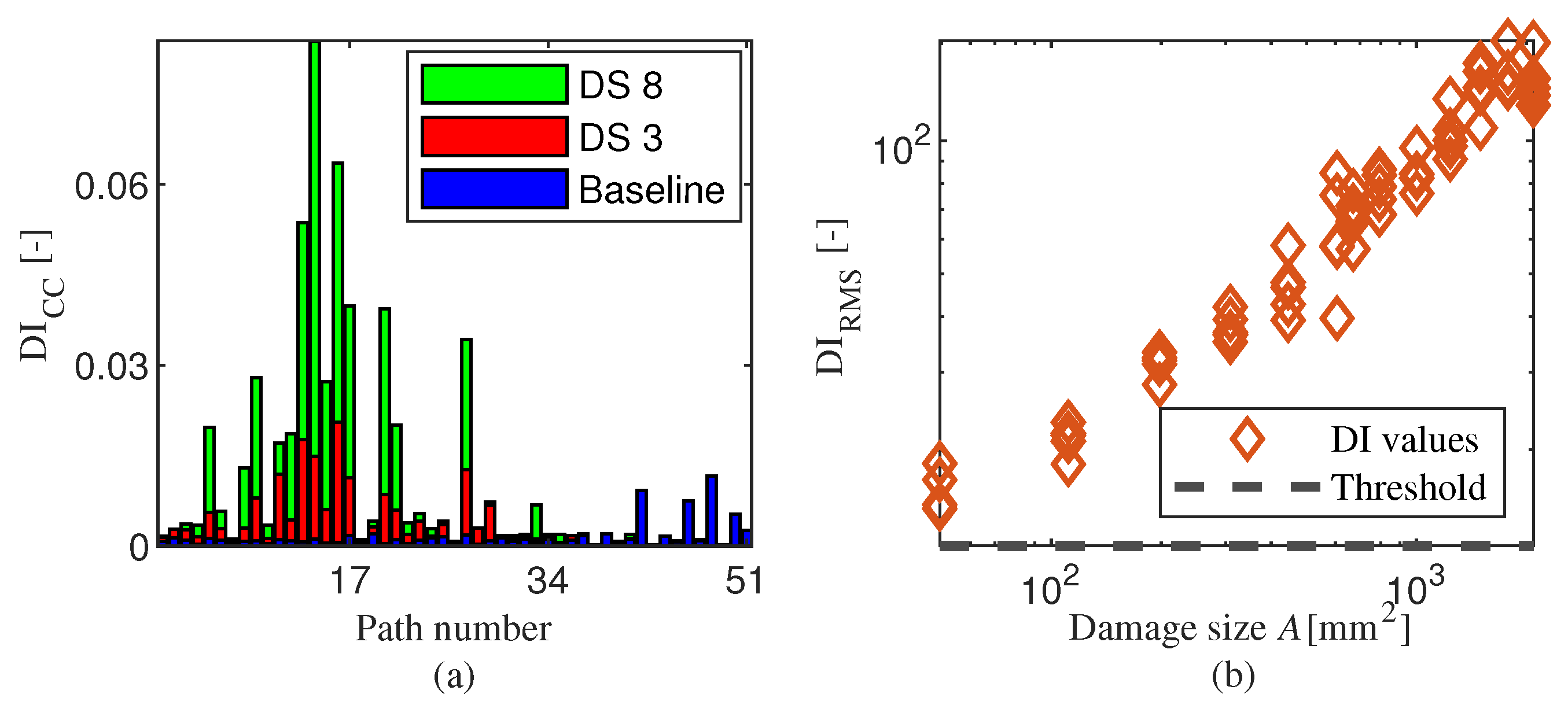
2.1. Level 1: Damage Detection

GWSHM systems are based on a permanently mounted transducer network; each path represents a transducer pair. To achieve detection, the measurement of different paths on the structure under monitoring needs to be evaluated. The most straightforward way to achieve this is by calculation of a path-based damage index, comparing between the pristine and damaged state [24]. Within this project, the correlation coefficient-based damage index ( D I C C , k ) between pristine and damage state of each kth path, i.e., transducer pair, has been evaluated:
D I C C , k = 1 i = 1 N S H , k , i S D , k , i i = 1 N S H , k , i i = 1 N S D , k , i i = 1 N S H , k , i 2 ( i = 1 N S H , k , i ) 2 . i = 1 N S D , k , i 2 ( i = 1 N S D , k , i ) 2 ,
where k = 1 , 2 , , N p is the path number, H is the damaged state, and D is the pristine one. N is the sampling points of the acquired signal. Essentially, this is 1 minus the correlation coefficient, which is approximately 1 for the undamaged state. Therefore, a damage index of 0 represents the undamaged state.
The calculation of D I C C , k results in multiple values for each measurement, one for each path. To result in one damage indicator, first these multiple values are placed in a vector ( D I C C ), then application of the ratio of root mean square values between the vector of correlation coefficient-based damage indices of the damage state and the baseline state results in the final damage indicator called D I R M S
D I R M S = 1 N p k = 1 N p D I C C 2 H 1 N p k = 1 N p D I C C 2 D .
In case only minor damage is present, the resultant value of D I R M S is expected to be small, as fewer paths close to the damage location will be influenced. The larger the damage, the more paths will be influenced, leading to a higher resultant value of D I R M S . Using this two-step technique to combine the multiple paths allows for only one threshold for a whole structure to be estimated.

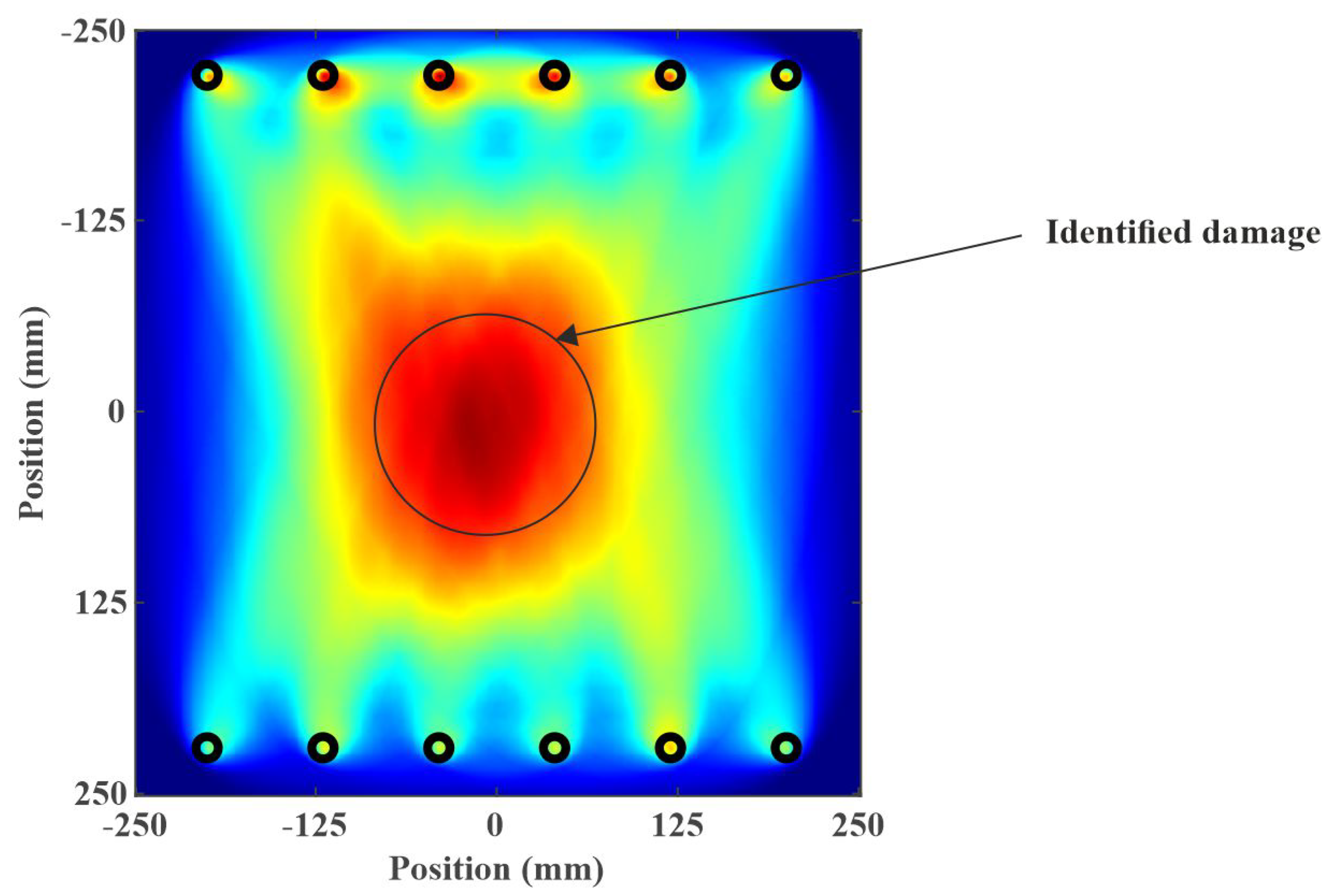
2.2. Level 2: Localization
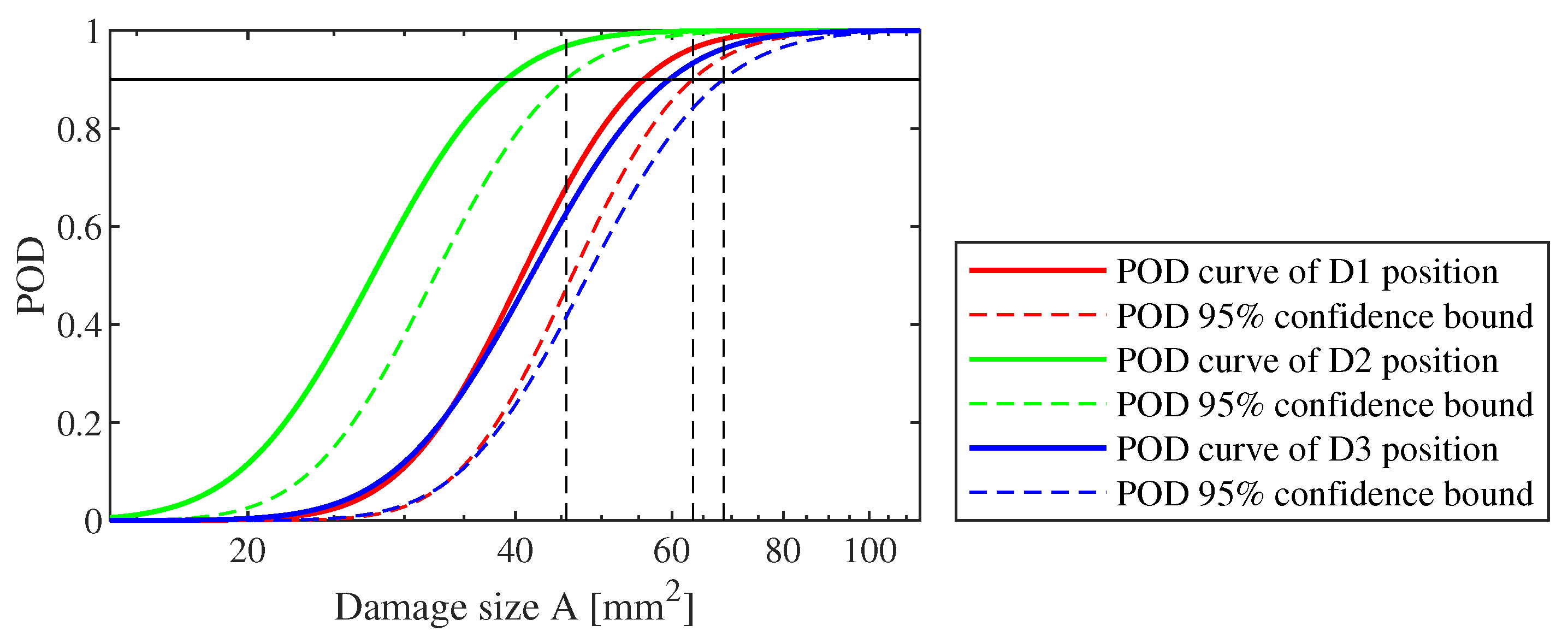
The signal correlation PDI algorithm [3] is used to determine the localization of damage. This algorithm calculates the intensity factor ( I ( x , y ) ) for each location on the plate based on D I C C , k values (1). I ( x , y ) of each pixel ( x , y ) is calculated:
I ( x , y ) = k = 1 N p ( D I C C , k ) 1 β 1 · R ( x , y ) + β β 1 ( k = 1 , 2 , , N p ; i , j = 1 , 2 , , N , b u t i j ) ,
where
R ( x , y ) = ( x x i ) 2 + ( y y i ) 2 + ( x x j ) 2 + ( y y j ) 2 ( x i x j ) 2 + ( y i y j ) 2 , when R ( x , y ) < β β , when R ( x , y ) > β
where β is a scaling parameter controlling the area influenced by transducer pairs (i.e., from the ith actuator located at ( x i , y i ) to jth sensor located at ( x j , y j )) and is set to 1.05 . Therefore, each path has an influence on the intensity factor for each pixel (x,y), but its influence is higher if the pixel is located on the path or in its vicinity. Finally, the higher the D I C C , k value for an actuator–sensor pair, the higher the probability of damage at the pixels near the kth path, as shown in Figure 1.
Within this paper, the way to estimate the I ( x , y ) at each pixel on the structure based on the signal correlation algorithm is slightly adapted, as a postprocessing of I ( x , y ) is performed to estimate a damage location with coordinates x and y. All the area that is in the vicinity and the transducers are not taken into account, as it is known that the I ( x , y ) values are naturally higher close to the transducer location. Moreover, the damage location is estimated to be at the center of the area with only the highest 5 % of the calculated field intensity values. As the damage locations for the experiment are known, this allows estimating a distance ( Δ d ). This is the distance between the known damage location and the estimated damage location. Based on this Δ d , the localization accuracy is established. As the damage size increases, it is expected that the Δ d value decreases.

2.3. POD Curve

The POD curve is used to estimate the damage detection capability of an SHM system for a defined setup and damage location. A 90 | 95 , P O D is the damage size that can be detected with a probability of detection of 90 % with a 95 % Wald confidence interval. A 90 | 95 , P O D is estimated using the established POD curve from Berens [25]. The typical procedure, considered to estimate A 90 | 95 , P O D using GWSHM system, consists of data processing, calculation of a system response a ^ , threshold determination based on undamaged training data, regression analysis, and POD curve generation.
Once a ^ values are calculated for damaged and undamaged measurements, a null hypothesis test using the Anderson–Darling methodology is carried out to ensure that a ^ values of the undamaged measurements are normally distributed [26]. Then, a probability of false alarm (PFA) is set to a defined value to determine the threshold value a ^ t h r e s h o l d . A functional relationship, preferably a linear relationship, between ( a ^ vs. a) is established by means of regression analysis. Within this calculation of the POD curve, a ^ is the damage indicator D I R M S , a is the area of the damage size, which is called damage size A , and a ^ t h r e s h o l d is the threshold value D I R M S , t h r e s h o l d :
D I R M S = m · f ( damage size A ) + b + τ 1 ,
frequently, log is used as function f for either one or both to achieve the necessary linear dependence. m and b are the slope and intercept of the linear relationship. τ 1 is the standard deviation of the scattering around the regression line. It is caused by parameters other than damage size A influencing D I R M S , such as temperature changes and different operational conditions. Then, the delta method, a statistical technique for deriving a variance of the model parameters, is applied to link the signal to POD curve. It is a transition from D I R M S vs. damage size A data to POD vs. damage size A data [27]. Regression analysis is used to estimate m, b and τ 1 to calculate σ P O D and μ P O D :
σ P O D = τ 1 m , μ P O D = D I R M S , t h r e s h o l d b m ,
hence, the POD curve can be generated as cumulative distribution function:
POD = f ( d a m a g e s i z e A ) μ P O D σ P O D
This POD curve is generated with a 50 % confidence bound. The 95 % confidence bound is achieved by computing the covariance matrix for the POD parameter ( σ and μ ). Finally, the A 90 | 95 , P O D value can be estimated:
A 90 | 95 , P O D = μ a | P O D = 90 % + z ( α ) σ a | P O D = 90 % .
For this case, z ( α ) is 1.645 and represents the confidence bound value of 95 % for on tailed standard normal distribution.
The final value, which is gained in this application, is the damage size A 90 | 95 , P O D at which damage will be detected with 90 % probability and at a confidence interval of 95 % .

2.4. Novel Method to Determine the Localization Accuracy

Using the parameter Δ d , it is assumed for a fixed damage location that the value Δ d decreases with increasing damage size A. The parameter Δ d can be estimated using the technique described in Section 2.2 but might also be the result of any other localization method. To determine and evaluate the localization accuracy for a given damage location, all values of Δ d vs. damage size A are used. It is expected to follow a negative linear trend as:
Δ d = n · log ( damage size A ) + c + τ 2 ,
where, n , and c are the slope and intercept of the linear relationship between Δ d and log ( damage size A ) . It is assumed and needs to be proven that the scattering around the regression line is independent of damage size A and, therefore, it consists of a normal distribution with its mean on the regression line and a standard deviation τ 2 , which needs to be determined from the data.
Similar to the POD analysis, as explained in Section 2.3, a statistical analysis leads to the probability of correct localization (POCL) curve, which helps to evaluate the localization accuracy. In many applications, a certain accuracy needs to be reached in order to use the method. This accuracy value, i.e., a fixed valued for Δ d , is called Δ d t h r e s h o l d .
Once the regression analysis is evaluated, σ P O C L and μ P O C L can be calculated:
σ P O C L = τ 2 n , μ P O C L = Δ d t h r e s h o l d c n ,
hence, the POCL curve can be generated as cumulative distribution function:
POCL = 1 f ( damage size A ) μ P O C L σ P O C L
Finally, the A 90 | 95 , P O C L value can be estimated:
A 90 | 95 , P O C L = μ a | P O C L = 90 % + z ( α ) σ a | P O C L = 90 % ,
calculating the 95 % confidence interval enables to determine the damage size A 90 | 95 , P O C L at which the Δ d is in 90 % of all the cases smaller than Δ d t h r e s h o l d .

3. Materials: OGW Platform

The experimental structure is a representative for a real aircraft component [28]. Its data set, analyzed within this paper, is available on the online platform Open Guided Waves (OGW) under ’guided wave basic measurement data for the plate with a stringer’.

3.1. Experimental Setup

A square plate of length 500 mm with a stiffening element in form of an omega stringer, both made of Carbon Fiber Reinforced Polymer (CFRP), is used as a structure, as shown in Figure 2a. The experimental setup is manufactured of prepreg Hexply® (Stamford, CT, USA) M 21 / 34 % / U K 134 / T 700 / 300 K for the plate and M 21 / 34 % / U D 194 / T 700 / I M A - 12 K for the omega stringer. The schematic illustration, shown in Figure 3a, shows the location of the co-bounded twelve piezoceramic transducers ( T 1 T 12 ) that are used for guided waves actuation and acquisition and the three chosen locations for reference damage placement (D1, D2, and D3), while Figure 3b shows a detailed design of the CFRP omega stringer attached to the square plate.
Pitch-catch signals for all transducer combinations at a constant temperature of 23 C and 50 % humidity are recorded. For this analysis, tone burst sine signal of five cycles Hann windowed with 40 kHz central frequency and a maximum amplitude of 100 V are excited, as shown in Figure 3c.

3.2. Reference Damage
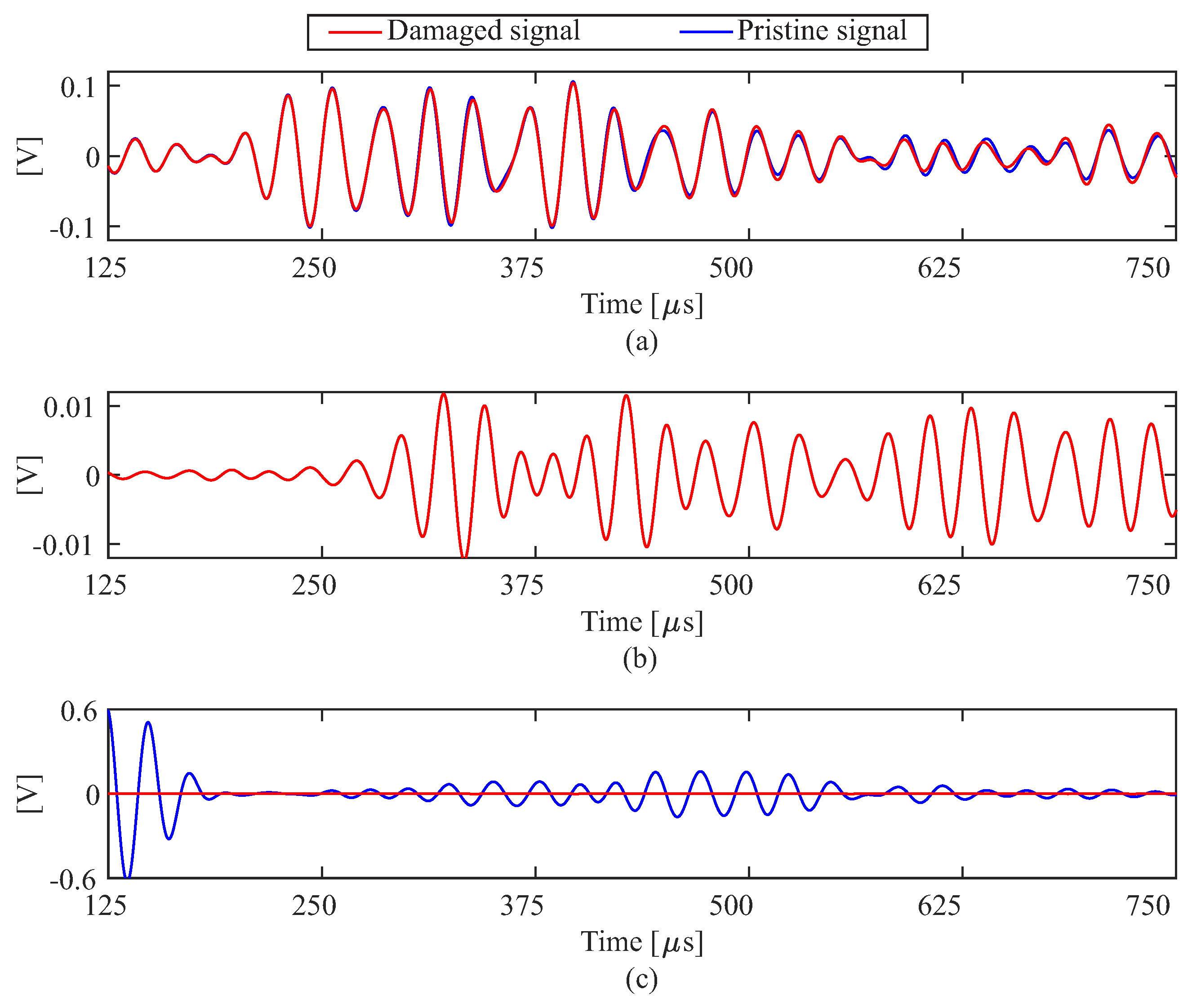
Thirteen elliptical steel discs with different damage size (DS) varied between (49.48–2090.53) mm 2 , as shown in Figure 2b, and have been attached individually to the CFRP structure by tacky tape. Adding mass to the structure causes a stiffness asymmetry by changing its geometry as well as it causes additional damping within its location. Despite its simplified shape, the interaction with guided waves leads to a decrease in amplitude, change in flight time, and mode conversion. The reference damage for each damage size was positioned at D1, D2, and D3, individually. While D1 and D3 are symmetric, D2 is located at a significant distance to the symmetry axes parallel to the omega stringer.
The authors are aware of the fact that this reference damage does not build a perfect model of a real delamination. Nevertheless, Bach et al. [29] have shown that the influence, especially on the guided waves crossing the damage, is similar for the reference damage and a real delamination.

3.3. Raw Data

The total data set of (OGW) platform [28] is 85 measurements recorded for several frequencies at each damage position ( D 1 D 3 ) . These measurements consist of 20 pristine measurements and 65 damaged ones (5 measurements for each damage size). Here, only the 40 kHz frequency is chosen. The postprocessing data analysis took place over a part of the signal, as shown in Figure 4a, after being filtered using a bandpass filter within (25–55 kHz). The first 125 μs of the recorded measurement are cross-talk between the channels while exciting the tone burst signal.
The estimated group velocity of the exciting signal propagating within the structure is roughly 1200 m/s. This indicates that A 0 -mode is mainly excited at 40 kHz [30]. Therefore, the time window of (125–750) μs is slightly longer than the time; a signal needs to start from the upright corner and end at the down right corner. This way, a compromise between taking into account a few reflections for short paths such as T 1 to T 6 and almost none for long paths, such as T 1 to T 12 , is realized.
As shown in Figure 4b, differential signal plays an essential role in clearly differentiating between the pristine and damaged state. It is a subtraction of a pristine measurement from a recorded measurement. If the recorded state is an undamaged one, the resultant differential signal amplitude is close to zero, while the amplitude of the damaged state differential signal is relatively high. Although 66 transducer pairs exist, 15 paths were excluded from the data analysis as they exhibit faulty measurements, only recording noise, as shown in Figure 4c.

4. Results: Reliability Assessment

The results shown in this section are related to an excitation of a tone burst signal at a central frequency of 40 kHz and five cycles. Even though the detection and localization figures are presented using only damage located at D1, the POD analysis and POCL curve figures are applied for D1, D2, and D3 locations.

4.1. Probability of Detection

As described in Section 2.1, a ^ v s . damage size A is estimated using a two-step approach to calculate a single system response D I R M S of a whole structure. The caluculated D I C C , k , which are used to calculate D I R M S , are shown vs. path number, in Figure 5a, for the damage sizes 8 and 3 as well as for the undamaged baseline. D I C C , k of the paths close to the damage are higher than others. A specific D I C C , k value for path k is increasing with increasing damage size, but more paths also start to see the effect of larger damage. Both effects play an important role. The D I R M S , as a ratio between the root mean square of vector D I C C of damaged vs. undamaged state, results in D I R M S v s . damage size A , also known as s y s t e m r e s p o n s e a ^ v s . damage size A , as shown in Figure 5b. It is clearly visible that the deviation around the linear interpolation is constant for all damage sizes A in l o g - l o g scale.
Once the D I R M S is calculated for the undamaged data set, a null hypothesis test is evaluated to prove its normal distribution. Finally, the threshold for the whole structure is estimated, with probability of false alarm ( P F A ) = 0.1 % , to a D I R M S value of 12.12 .
The POD curves, generated according to Section 2.3, for damage located at D1, D2, and D3 are shown in Figure 6. The damage size A axis is presented in a log scale, while the POD axis is a linear scale. The solid lines, in red, blue, and green, are related to the POD curves with a confidence bound of 50 % . Meanwhile, the dashed lines in the same colors are related to increasing the confidence bound to 95 % .
A 90 | 95 , P O D values are obtained from the POD curves and presented in mm 2 in Table 1. A 90 | 95 , P O D values provide information regarding the smallest damage size A that can be detected with a probability of 90 % and confidence bounds 95 % .

4.2. Localization Accuracy

For the chosen probability-based diagnostic imaging technique based on signal correlation algorithm, the D I C C , k of all 36 paths, crossing the omega stringer, are chosen. A resulting image is produced as shown in Figure 7a.
The red cross represents the estimated damage location of DS 13 for damage located at D1, while the green cross represents the actual damage location. The yellow area represents the highest 5 % of the I ( x , y ) , while all areas with lower values are set to zero for this visualization.
The distance ( Δ d ) is estimated for all recorded states and their repetition. Its trend is a negative linear trend, as shown in Figure 7b. A null hypothesis test using Anderson–Darling methodology is evaluated to ensure the normal distribution of Δ d values at each damage size A . Finally, the desired Δ d t h r e s h o l d , for damage located at D1, D2, and D3, has chosen to be 8 cm.
The probability of correct localization (POCL) curves for damage located at D1, D2, and D3 are generated and shown in Figure 8. Red, green, and blue solid lines are the generated POCL curves with a confidence bound 50 % . Increasing the confidence bound to 95 % results in shifting the POCL curves to the right, as shown in dashed lines with the same colors. The generated POCL curves provide information regarding the probability of correct localization versus the damage size A. Moreover, it is possible to determine A 90 | 95 , P O C L values as presented in Table 2. In such case, A 90 | 95 , P O C L values provide information regarding the smallest damage size A that can be reliably localized within 8 cm with a probability of 90 % and 95 % confidence bounds. Regarding POCL curves, the larger the damage size A, the more accurate the estimated damage location using the signal correlation PDI algorithm for localizing the damage. It should be noted that, to retain the comparability regarding the statistical analysis, the POCL probability is plotted in reverse, having the 0 at the top.

5. Discussion

The resultant POD curves provide information regarding the smallest damage size A that can be reliably detected for three damage locations. The POCL curves provide information regarding the smallest damage size A at which a defined accuracy level can be reached for the defined three damage locations.
Regarding damage located at D1 and D3, the POD and POCL curves for detection and localization show similar results. The A 90 | 95 , P O D and A 90 | 95 , P O C L values have only a small difference, while damage located at D2 provides different results. The A 90 | 95 , P O D value is lower for D2 than those of D1 and D3 for detection level, while A 90 | 95 , P O C L value is larger for localization level.
The reasons for this are caused by the chosen setup and the chosen algorithms for detection and localization. All paths have been used for the detection level, including those that did not cross the stringer. Their D I C C , k values already tend toward being high. This leads to D2 being detected at lower damage sizes A with a high probability and confidence. Due to the symmetric set up, the A 90 | 95 , P O D and A 90 | 95 , P O C L values for damage located at D1 and D3 are in the same range. As expected, the results show that it is not possible to assume that a better detection ability is correlated with a better localization accuracy. Therefore, it is necessary to evaluate the localization accuracy separately.
The proposed procedure to determine the localization accuracy has a high location dependence for the chosen algorithm. Even for all the D I C C , k being relatively high, the I ( X , y ) values would be highest in the center of the plate and virtually along the axis of the stringer, as only the path which crosses the omega stringer is taken into account. Due to this fact, D1 and D3, which are closer to the stringer, have better POCL curves and smaller A 90 | 95 , P O C L values.
Technically, the two-step technique as well as the localization technique can detect a larger number of damage occurring simultaneously in different positions. The given form of POD and POCL techniques show location dependent results and, therefore, it is evaluated for one damage at a time.

6. Conclusions

Within this paper, the POD and POCL curves are generated to assess the location dependent probability of detection using a two-step technique and the localization accuracy using the signal correlation algorithm for a given setup and data set. The detection probability does not necessarily correlate to a better localization accuracy, as shown for the three damage locations. The detection probability and localization accuracy show similar results for damage closer to the center of the sensor arrays (D1 and D3). As the distance increases between the damage location and center of the sensor array, which coincides with the symmetry of the added omega stringer, the sensitivity of detection increases, while localization sensitivity deteriorates. Despite the high number of transducer paths, the two-step technique used to detect the damage generates only one POD curve to assess the GWSHM system. On the other hand, the novel method to determine localization accuracy has the capability to quantify the smallest damage size that can be reliably localized with a chosen localization accuracy.

Author Contributions

Conceptualization, A.B., T.M. and I.M.; methodology, A.B., T.M. and I.M.; software, A.B., T.M. and I.M.; validation, A.B., T.M. and I.M.; formal analysis, A.B. and T.M.; investigation, A.B.; resources, I.M.; data curation, A.B. and T.M.; writing—original draft preparation, A.B.; writing—review and editing, A.B. and I.M.; visualization, A.B. and I.M.; supervision, I.M.; funding acquisition, I.M. All authors have read and agreed to the published version of the manuscript.

Funding

This research was funded by GW4SHM, EU Horizon 2020 H2020-MSCA-ITN-2019, Grant No. 860104.

Institutional Review Board Statement

Not applicable.

Informed Consent Statement

Not applicable.

Data Availability Statement

The used raw data is available on the website openguidedwaves.de, accessed on 10 October 2021. The processed full data set of this study is available from the authors upon reasonable request.

Acknowledgments

The Authors thank Thomas Vogt for his valuable comments upon results.

Conflicts of Interest

The authors declare no conflict of interest.

References

  1. Cawley, P. Structural health monitoring: Closing the gap between research and industrial deployment. Struct. Health Monitor. 2018, 17, 1225–1244. [Google Scholar] [CrossRef] [Green Version]
  2. Farrar, C.R.; Worden, K. An introduction to structural health monitoring. Philos. Trans. R. Soc. A Math. Phys. Eng. Sci. 2007, 365, 303–315. [Google Scholar] [CrossRef] [PubMed]
  3. Su, Z.; Ye, L. Identification of Damage Using Lamb Waves: From Fundamentals to Applications; Springer Science & Business Media: Berlin, Germany, 2009; Volume 48, pp. 171–200. [Google Scholar]
  4. Mandache, C.; Genest, M.; Khan, M.; Mrad, N. Considerations on structural health monitoring reliability. In Proceedings of the International Workshop Smart Materials, Structures & NDT in Aerospace, Montreal, QC, Canada, 2–4 November 2011; Volume 24. [Google Scholar]
  5. Monaco, E.; Memmolo, V.; Ricci, F.; Boffa, N.D.; Maio, L. Guided waves based SHM systems for composites structural elements: Statistical analyses finalized at probability of detection definition and assessment. In Proceedings of the Health Monitoring of Structural and Biological Systems 2015, San Diego, CA, USA, 9–12 March 2015; International Society for Optics and Photonics: San Diego, CA, USA, 2015; Volume 9438, p. 1. [Google Scholar]
  6. Grooteman, F. Damage detection and probability of detection for a SHM system based on optical fibres applied to a stiffened composite panel. In Proceedings of the International Conference on Noise and Vibration Engineering, Leuven, Belgium, 17–19 September 2012; pp. 3317–3330. [Google Scholar]
  7. Kelly, D.W.; Scott, M.L.; Thomson, R.S. Composite Aircraft Structures. In Modeling Complex Engineering Structures; American Society of Civil Engineers: Reston, VA, USA, 2007; pp. 247–274. [Google Scholar]
  8. Rentala, V.K.; Mylavarapu, P.; Gautam, J.P. Issues in estimating probability of detection of NDT techniques—A model assisted approach. Ultrasonics 2018, 87, 59–70. [Google Scholar] [CrossRef] [PubMed]
  9. Annis, C.; Bray, E.; Hardy, H.; Hoppe, P.M.S. Nondestructive Evaluation System Reliability Assessment; Handbook MIL-HDBK-1823A; United States Department of Defense, Wright-Patterson AFB: Dayton, OH, USA, 2009. [Google Scholar]
  10. Georgiou, G.A. PoD curves, their derivation, applications and limitations. Insight-Non-Destruct. Test. Cond. Monit. 2007, 49, 409–414. [Google Scholar] [CrossRef]
  11. Zhang, R.; Mahadevan, S. Fatigue reliability analysis using nondestructive inspection. J. Struct. Eng. 2001, 127, 957–965. [Google Scholar] [CrossRef]
  12. Cobb, A.C.; Michaels, J.E.; Michaels, T.E. Ultrasonic structural health monitoring: A probability of detection case study. AIP Conf. Proc. 2009, 1096, 1800–1807. [Google Scholar]
  13. Janapati, V.; Kopsaftopoulos, F.; Li, F.; Lee, S.J.; Chang, F.K. Damage detection sensitivity characterization of acousto-ultrasound-based structural health monitoring techniques. Struct. Health Monit. Int. J. 2016, 15, 143–161. [Google Scholar] [CrossRef]
  14. Gianneo, A.; Carboni, M.; Giglio, M. Feasibility study of a multi-parameter probability of detection formulation for a Lamb waves-based structural health monitoring approach to light alloy aeronautical plates. Struct. Health Monit. Int. J. 2016, 16, 225–249. [Google Scholar] [CrossRef]
  15. Mueller, I.; Fritzen, C.P. Inspection of piezoceramic transducers used for structural health monitoring. Materials 2017, 10, 71. [Google Scholar] [CrossRef] [PubMed] [Green Version]
  16. Ihn, J.B.; Pado, L.; Leonard, M.S.; Olson, S.E.; DeSimio, M.P. Development and Performance Quantification of an Ultrasonic Structural Health Monitoring System for Monitoring Fatigue Cracks on a Complex Aircraft Structure; Technical Report; Air Force Research Lab Wright-Patterson Afb Oh: Dayton, OH, USA, 2011. [Google Scholar]
  17. Schneider, C.R.; Rudlin, J.R. Review of statistical methods used in quantifying NDT reliability. Insight-Non-Destruct. Test. Cond. Monit. 2004, 46, 77–79. [Google Scholar] [CrossRef]
  18. Tschöke, K.; Mueller, I.; Memmolo, V.; Moix-Bonet, M.; Moll, J.; Lugovtsova, Y.; Golub, M.; Venkat, R.S.; Schubert, L. Feasibility of Model-Assisted Probability of Detection Principles for Structural Health Monitoring Systems Based on Guided Waves for Fiber-Reinforced Composites. IEEE Trans. Ultrason. Ferroelectr. Freq. Control 2021, 68, 3156–3173. [Google Scholar] [CrossRef] [PubMed]
  19. Tanaka, H.; Sharif Khodaei, Z. Reliability assessment of SHM methodologies for damage detection. In Key Engineering Materials; Trans Tech Publ.: Stafa, Switzerland, 2016; Volume 713, pp. 244–247. [Google Scholar]
  20. Zhou, C.; Su, Z.; Cheng, L. Quantitative evaluation of orientation-specific damage using elastic waves and probability-based diagnostic imaging. Mech. Syst. Signal Process. 2011, 25, 2135–2156. [Google Scholar] [CrossRef]
  21. Liu, K.; Ma, S.; Wu, Z.; Zheng, Y.; Qu, X.; Wang, Y.; Wu, W. A novel probability-based diagnostic imaging with weight compensation for damage localization using guided waves. Struct. Health Monit. 2016, 15, 162–173. [Google Scholar] [CrossRef]
  22. Liu, B.; Liu, T.; Lin, Y.; Zhao, J. An aircraft pallet damage monitoring method based on damage subarea identification and probability-based diagnostic imaging. J. Adv. Transp. 2019, 2019, 2568736. [Google Scholar] [CrossRef]
  23. Liu, G.; Wang, B.; Wang, L.; Yang, Y.; Wang, X. Probability-based diagnostic imaging with corrected weight distribution for damage detection of stiffened composite panel. Struct. Health Monit. 2021, 14759217211033967. [Google Scholar] [CrossRef]
  24. Moix-Bonet, M.; Wierach, P.; Loendersloot, R.; Bach, M. Damage assessment in composite structures based on acousto-ultrasonics—Evaluation of performance. In Smart Intelligent Aircraft Structures (SARISTU); Springer: Berlin, Germany, 2016; pp. 617–629. [Google Scholar]
  25. Berens, A.P. NDE reliability data analysis. ASM Handb. 1989, 17, 689–701. [Google Scholar]
  26. Lewis, P.A. Distribution of the Anderson-Darling statistic. In Annals of Mathematical Statistics; Institute of Mathematical Statistics: Beachwood, OH, USA, 1961; pp. 1118–1124. [Google Scholar]
  27. Schubert Kabban, C.M.; Greenwell, B.M.; DeSimio, M.P.; Derriso, M.M. The probability of detection for structural health monitoring systems: Repeated measures data. Struct. Health Monit. 2015, 14, 252–264. [Google Scholar] [CrossRef]
  28. Moll, J.; Kexel, C.; Kathol, J.; Fritzen, C.P.; Moix-Bonet, M.; Willberg, C.; Rennoch, M.; Koerdt, M.; Herrmann, A. Guided waves for damage detection in complex composite structures: The influence of omega stringer and different reference damage size. Appl. Sci. 2020, 10, 3068. [Google Scholar] [CrossRef]
  29. Bach, M.; Pouilly, A.; Eckstein, B.; Bonet, M.M. Reference damages for verification of probability of detection with guided waves. In Structural Health Monitoring 2017; Destech Publications: Lancaster, PA, USA, 2017. [Google Scholar] [CrossRef]
  30. Moll, J.; Kathol, J.; Fritzen, C.P.; Moix-Bonet, M.; Rennoch, M.; Koerdt, M.; Herrmann, A.S.; Sause, M.G.; Bach, M. Open guided waves: Online platform for ultrasonic guided wave measurements. Struct. Health Monit. 2019, 18, 1903–1914. [Google Scholar] [CrossRef]
Figure 1. Signal correlation algorithm: map of damage based on correlation algorithm of captured lamb wave signals.
Applmech 02 00058 g001
Figure 2. (a) Photo of the square plate with the omega stringer. (b) Visualization of the thirteen reference damages fabricated for the case study [28].
Applmech 02 00058 g002
Figure 3. (a) Schematic illustration of the location of the 12 transducers on the plate with stringer and the three different locations of the damage. (b) Schematic illustration of the omega stringer (dimensions in mm). (c) The excited tune burst sine signal of 5 cycle Hann windowed with a central frequency of 40 kHz [28].
Applmech 02 00058 g003
Figure 4. (a) The difference between the damaged signal and the pristine one. (b) The differential signal: subtraction of the damaged signal and pristine signal from a baseline signal. (c) Fault measurement: some recorded transducer pairs recorded only noise.
Applmech 02 00058 g004
Figure 5. (a) First step: calculation of D I C C , k . The resultant plot represents the effect of damage on each path. (b) Second step: calculation of D I R M S . The resultant plot represents only one value for each recorded measurement.
Applmech 02 00058 g005
Figure 6. POD curves for increasing reference damage size A located at D1, D2, and D3 using the two-step analysis technique.
Applmech 02 00058 g006
Figure 7. (a) Postprocessed I ( x , y ) map for the largest reference damage size, enabling the estimation of damage location. The resultant distance ( Δ d ) is highly dependent on damage size and damage location. (b) Estimation of Δ d values of all measurements at damage location D1 over damage size A. First step for determining the accuracy of localization.
Applmech 02 00058 g007
Figure 8. POCL curves for reference damage located at D1, D2, and D3 using signal correlation algorithm.
Applmech 02 00058 g008
Table 1. A 90 | 95 , P O D values in mm 2 .
D1D2D3
63.345.668.5
Table 2. A 90 | 95 , P O C L values in mm 2 .
D1D2D3
106326126
Publisher’s Note: MDPI stays neutral with regard to jurisdictional claims in published maps and institutional affiliations.

