Article

Response-Only Damage Detection Approach of CFRP Gas Tanks Using Clustering and Vibrational Measurements

by
Ilias Zacharakis
and
Dimitrios Giagopoulos
*
Department of Mechanical Engineering, University of Western Macedonia, 50100 Kozani, Greece
*
Author to whom correspondence should be addressed.
Appl. Mech. 2021, 2(4), 1057-1072; https://doi.org/10.3390/applmech2040061
Submission received: 18 October 2021 / Revised: 1 December 2021 / Accepted: 9 December 2021 / Published: 11 December 2021
(This article belongs to the Special Issue Damage Sensing in Composites for Structural Health Monitoring)

Abstract

:
The advancements in the automotive, aviation, and aerospace industry have led to an increased usage of CFRP high-pressure gas tanks. In order to avoid any fatal accidents, the inspection procedures require accuracy, but also practicality, to be used in the industry. The presented work focuses on response-only metrics from vibrational experimental measurements of the CFRP tank. The power spectral density and transmittance function curves are both compared for the accuracy and ability to be used as metrics for damage detection. Along with the selection of the proper metric, an appropriate clustering algorithm that can accurately group similar states of the structure is of high importance. Two clustering algorithms, agglomerative hierarchical and spectral clustering, are employed and compared for their performance. A small Type V CFRP tank is used as an experimental structure on this benchmark problem. In order to create realistic material damage, the tank is placed on an impact system multiple times where different damage magnitudes are created. After each new state and damage magnitude on the tank, vibrational experimental data are collected. Using the collected data, all the combinations of the mentioned metrics and algorithms are executed and properly compared to evaluate their accuracy.

1. Introduction

The evolution of aerospace and aviation systems and also the swiftness of the automotive industry to adopt different types of fuels has led to an increasing interest in carbon fiber reinforced polymer composite (CFRP) tanks [1]. The characteristics of the high strength of the materials, leading to high internal pressure capabilities, and the low weight ratio have made these types of tanks a prime candidate for advanced applications. Automotive applications include the storage of hydrogen or liquified natural gas under high internal pressure [2,3]. The aerospace and aviation industry has long seen their applications as a weight-reducing solution, such as for liquid and gaseous oxygen [4] and other fuel storage.
The CFRP materials have great advantages over common structural materials such as metal. Despite their good strength characteristics, CFRP materials using epoxy matrix are prone to impact damage [5]. Cracks and delamination can occur within the material while remaining unnoticed by the human eye. During continuous usage, this can lead the damage to progress within the material and eventually destroy it without warning. Regarding applications using CFRP high-pressure tanks, this can lead to catastrophic failure. Besides the high internal pressure, the contents of the tank are usually dangerous and flammable. The continuous high internal pressure and the cyclic loading from refueling can lead to quick progression of any damage, and even fatal accidents.
Many inspection methodologies (non-vibration-based) have been proposed for CFRP structures. Infrared thermography has been proposed to detect impact damage in CFRP plates [6], and acoustic and ultrasonic techniques have been presented to inspect or monitor damage to CFRP tanks and simple plates [7,8,9] and eddy current methods [10].
The vibration-based approach is a subcategory of structural health monitoring (SHM) methods that rely on the fact that structural damage will affect the dynamic characteristic of a structure. One of the advantages of vibration-based methods is that they do not rely on properties such as electric and acoustic conductivity. More traditional vibration-based methods would emphasize the changes of natural frequencies, mode shapes, and autoregressive model (AR) coefficients [11]. Other methods rely on finite element (FE) models to indicate the damage, and have been applied to composite and metallic structures [12,13,14]. While the requirement for an FE model can be a drawback, it can be resolved using model updating procedures that will produce high fidelity FE models, even for CFRP structures that use simplified equivalent materials to model the composite [15,16,17]. Recent trends show an increasing interest in the use of machine learning (ML) for SHM systems [18,19,20,21] that rely on experimentally measured data or artificially collected data [22,23] to properly train the ML model for classification.
The presented work focuses on the use of response-only metrics from vibrational experimental measurements. Most of the mentioned vibration-based works rely on modal characteristics and frequency response functions (FRFs). Using output metrics alone, there is no need to record the input excitation, thus making the experimental setup simpler. Two metrics are compared in the following sections. The first is the power spectral density (PSD) and has been used for SHM purposes in the past [24,25]. The second metric is the transmittance function (TF) [26,27]; while it is prone to material changes and it is independent of the input excitation of the experiment, its usage is limited in the literature.
The following approach is intended for application on the inspection of a large number of identical objects. It is tested on a CFRP tank as its usage is not restricted. In order to identify the status of the tank, a clustering algorithm is applied that forms groups of similar experimental tests. Clustering algorithms in various forms have been applied in the past for damage detection [28,29]. In the following sections, two clustering algorithms are compared for their applicability and efficiency. The first is the agglomerative hierarchical clustering algorithm [29,30,31,32] that relies on the construction of a binary tree based on the differences between observations. The second is the spectral clustering algorithm [33,34,35,36], which is based on graph theory and constructs a similarity graph with the experimental observations. Using this similarity graph and the corresponding matrix representation (similarity matrix), it calculates its Laplacian matrix. From the eigenvalues of the Laplacian matrix, it is able to cluster similar data together. As will be presented in the following sections, both the metrics and clustering algorithms do not perform with the same accuracy.
Prior to any inspection, a small database is needed. It must include measurements from healthy and damaged tanks. During an inspection, these algorithms can be used with small computational effort, as both can support incremental computations. This means that the acquired clustered database can be stored, and when new measurements are available, only the pairwise distances of the new data sets must be computed. As the inspection of different states is continued, the more accurate the algorithm will be. It must be noted that some limitations always apply. The following procedure is tested on a CFRP tank with a simple structure, as it has no moving parts, no bolted connections, etc. While this can be applied to other, similar structures as well, if a structure is complex, it is advised that other algorithms are also tested.
This work is organized as follows. Section 2 describes the working principles of both the clustering algorithms and the modifications needed to apply the algorithms. Section 2 also provides the details of the PSD and transmittance function. Section 3 presents the details of the experimental setup with the CFRP tank. Section 3.1 describes the creation of the damaged area using an impact system and visualizes the damage result on the PSD and transmittance curves. Following this, Section 3.2 presents the final comparison between all of the different metrics and algorithms. Finally, the conclusions are summarized in Section 4.

2. Clustering

Clustering is an explanatory analysis method that aims to discriminate data sets into groups (clusters) of objects with high similarity. It is an unsupervised method that, in the context of damage detection, can be used on two tasks depending on the available data. The first task is to separate the data sets between tanks in healthy and damaged states. The second task is to create clusters of similar damage types or magnitude. This might be more desirable in some cases, as it requires more available experimental data for different damaged states. While in the present work only experimental data are examined, the data availability drawback could be surpassed by hybrid approaches also using simulated data of damaged cases [22,23].
The hierarchical clustering and spectral clustering algorithms are applied in the following sections for comparison. Both algorithms rely on the pairwise distance between observations. These are general clustering algorithms and are available on many software packages such as scikit-learn [37] and MATLAB [38].

2.1. Hierarchical Clustering

Hierarchical agglomerative clustering relies on building a binary tree, starting from the leaves (single data element) and continuing by merging the two closest elements into subclusters. This process iterates by creating higher-level clusters from the existing ones until the tree reaches the root, which contains all of the data sets [30]. The distance between two subclusters is called the linkage distance. Based on this linkage distance, the whole tree is constructed.
Given a number of data sets, the procedure of hierarchical clustering can be summarized by the following steps [29,31,32]:
  • Evaluation of the pairwise distance of the data sets.
    More details on the calculation of this step are referred to in Section 2.3.
  • Construct the hierarchical binary tree.
    In this step, similar pairs of points are merged into a cluster. Iteratively, these clusters are merged again to construct higher-level clusters until the tree is fully developed. The criterion for merging is the distance metric.
    Several different methods exist to achieve this procedure, such as the single linkage, complete linkage, and average linkage approaches [39]. In the present work, the complete linkage method is considered. With this method, any point to be included in an existing cluster must be within a certain level of similarity to all members of that cluster.
Let q and r be two clusters with n number of objects each. The complete linkage (distance between two clusters) can be computed using Equation (1).
d ( q , r ) = max ( d i s t ( x i q , x i r ) ) ,     1 i n
3.
Cut the tree into the specified number of clusters. The number of clusters is an input variable.

2.2. Spectral Clustering

Spectral clustering is a method with roots in graph theory. Given the available data sets, it involves the constructions of a similarity graph, finding its Laplacian matrix, and using this matrix to find a k number of eigenvectors in order to split the graph in k ways.
A number of modifications of this algorithm have been presented in the past [33,34,35,36]. In the present work, the normalized spectral clustering algorithm proposed by Shi and Malik is applied [35].
The main steps of the spectral clustering algorithm are the following:
  • Let X = x 1 , x 2 , , x n be the collection of observations, where n is the total number of observations, and x is a set of variables. Each variable can be a single data point or, with proper modifications, it can be a set of data points. In the context of this work, a variable inside x is treated as a collection of data points, as it represents a curve on the frequency domain.
  • Using the selected distance function, the pairwise distance ( D i s t ) is calculated between all n observations.
  • Construction of the similarity matrix. Using the D i s t n × n matrix, the elements of row i and column j of the similarity matrix can be calculated using Equation (2). The similarity matrix is the matrix representation of the graph.
    S i , j = exp ( ( D i s t i , j σ ) 2 )
  • Calculate the unnormalized Laplacian matrix using Equation (3):
    L = D g S
    where D g , degree matrix, is a diagonal matrix calculated by the sum of the rows of the similarity matrix. As such, the m -th diagonal element is calculated using Equation (4).
    D g ( m , m ) = j = 1 n S i , j
  • Calculate the normalized Laplacian matrix using Equation (5).
    L n o r m = D g 1 L
  • Solve the eigenvalue problem and calculate the first k numbers of eigenvectors. Let U n × k be the matrix containing the eigenvectors (as columns).
  • Use each row of U n × k as a point and cluster with the k-means algorithm.
  • Finally, group the original points in X along with the points of the corresponding row of U n × k .

2.3. Metric of Comparison

The present work focuses on response-only approaches. Using vibrational acceleration measurements, two different metrics are compared for their effectiveness.
The first metric is the power spectral density (PSD), S r , of the acceleration response signal. The PSD is highly correlated with the magnitude of excitation. Therefore, to effectively apply the clustering algorithms, the experimental procedure must always include the same magnitude of excitation. In the present work, Welch’s method is used for the estimation of the PSD.
The second metric is the transmittance function (TF). It is expressed as the ratio of the cross-spectral density (CSD), S r s , between two acceleration response signals, over the auto-spectral density, S r r , and can be calculated using Equation (6):
T r s ( ω ) = S r s ( ω ) S r r ( ω ) = x ¨ r ( ω )    x ¨ s * ( ω ) x ¨ r ( ω )    x ¨ r * ( ω )
where x ¨ ( ω ) is the Fourier transformation of the acceleration signal and x ¨ * ( ω ) its complex conjugate, while ω is the frequency and subscripts r , s denote the degrees of freedom.
The TF is a relative measure between two acceleration signals. If q is the number of signals used, a matrix of all possible combinations is:
T = [ 1 T 12 T 1 q T 21 1 T 2 q T q 1 T q 2 1 ] q × q
Only the unique combinations from Equation (7) are necessary to be calculated, as the rest contain the same information with their corresponding symmetric element. Other researchers propose the use only from sequential TFs that correspond to the first upper diagonal of the T matrix [26,40,41]. In the present work, all the unique combinations of the matrix are used that correspond to the upper triangular part of the T matrix. Furthermore, as the structure can be further analyzed in three dimensions, the T matrix can be divided into three axis-specific matrices in the global coordinate system. For example, if w is the number of triaxial acceleration sensors, the divided TF matrices for the X-, Y-, and Z-axis can be expressed as Equation (8):
T X = [ 1 T 12 X T 1 w X T 21 X 1 T 2 w X T w 1 X T w 1 X 1 ] w × w T Y = [ 1 T 12 Y T 1 w Y T 21 Y 1 T 2 w Y T w 1 Y T w 1 Y 1 ] w × w T Z = [ 1 T 12 Z T 1 w Z T 21 Z 1 T 2 w Z T w 1 Z T w 1 Z 1 ] w × w
The transmittance function is a relative measure between two acceleration signals; thus, it is independent of the excitation magnitude. This is a serious advantage during the testing procedure of a large number of identical structures. While the TF is not dependent on the excitation magnitude, for the sake of a proper comparison, the same excitation magnitude will be examined in all cases.
Both PSD and TF measures exist in the frequency domain. The selected clustering algorithms rely on pairwise distances between the observations (data set states). As each variable on a given observation is a series of data values and a curve on the frequency domain, the proper modifications were made to the algorithms in order to calculate the distances needed.
If V represents a variable, which is a curve on the frequency domain, the calculation of the distance between two variables of observations k ,    q is presented in Equation (9), where f 1 , f 2 represent the frequency range of interest and f s t e p s are the total frequency points of the curve.
J = ( f 1 f 2 ( V k V q ) 2 f s t e p s )
The total distance—Equation (10) —of the two observations k ,    q can be expressed as the mean value of all the J distances, as in Equation (9), where ν is the total number of J distances between observation k and q .
D i s t ( k , q ) = m e a n ( J 1 ( k , q ) , J 2 ( k , q ) , , J v ( k , q ) )
To construct the pairwise distance matrix, Equation (10) is used iteratively for all available observations.

3. Type V CFRP Tank Impact Damage

The experimental structure is a linerless (Type V) high-pressure tank made from carbon fiber reinforced polymer composite material. Type V CFRP tanks do not include an internal plastic or aluminum liner. Commonly, these tanks are manufactured with the filament winding technique. During the manufacturing, the mandrel is detached and only the CFRP material remains on the tank’s wall, along with the aluminum endings. This procedure gives the ability to reduce the weight even more.
Figure 1 presents the tank during the filament winding process. This photo was taken prior to the composite curing process inside an oven. After the curing process was complete, the mandrel, which now holds the shape of the tank, was removed.
The experimental setup consisted of a CFRP Type V tank with one end fixed directly on an electrodynamic shaker. The internal diameter of the tank was 200 mm, with a maximum wall thickness of 4 mm and a total length (with the aluminum parts) of 680 mm. Upon the tank, four triaxial accelerometers were placed at different locations. The BK 4535-B-001 type of accelerometer was used, which has a frequency range of 0.3–10,000 Hz and a mass of only 6 g. It must be noted that due to the thickness of the CFRP material and the weight of the structure (5 kg approx.), the mass of the acceleration sensors was not expected to affect the results.
Figure 2 presents the experimental setup of the tank, along with a sketch of the location of the accelerometers. More specifically, the figure shows two of the four placed accelerometers, A1 and A2, with their corresponding height from the bottom of the tank (H1 and H2). The accelerometer’s location details are presented in Table 1. The angle between the accelerometer was measured with a right-hand rule, starting from accelerometer A1.
The location and number of acceleration sensors were evaluated by the eigenmodes of the structure. A finite element model of the structure was developed using the commercial software package MSC Nastran. The indicative eigenmodes from the modal analysis of the model between the range of 0 and 1500 Hz are presented in Figure 3.
The excitation was set as a random signal and applied in the X-axis with the same magnitude for every experimental test. All tests had the same duration of 5 s and a sampling rate of 5120 Hz. The experimental measurements that are considered for the clustering are only from the X-axis. Prior to any damage to the tank, experimental measurements were executed on those in a healthy state.

3.1. Impact Damage

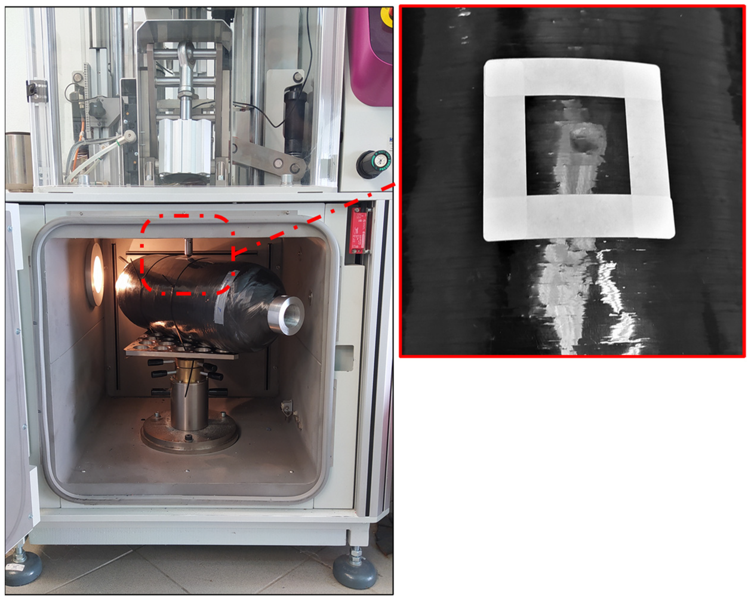
During the transfer, usage, and installation of high-pressure tanks, many kinds of impact scenarios could occur. To properly cause impact damage, an INSTRON CEAST 9350 drop tower impact system was used. The impact system uses a small circular beam head with a round edge 20 mm in diameter. The tank was placed on the closed chamber of the machine and tied to prevent any movement. The system’s head hit the tank with a total energy of 10 joules at a predefined location on the middle of the tank’s length.
It must be noted that the tank weighs around 5 kg when empty. In the scenario that this tank is falling from a person’s hands during a transfer, the total energy produced is higher than 10 joules. After the first impact, the tank was placed on the electrodynamics shaker with the same setup, and the first set of experimental measurements was acquired. The same procedure was repeated four times in total. The same tank was damaged with the same energy at the same location. Each time, the material was degraded even more. After each impact hit, the tank was placed on the electrodynamic shaker to acquire a set of experimental measurements of the current state.
Figure 4 presents the impact setup on the isolated chamber. The magnified area is the impact location after the last hit. The impact location rests on the middle of the tank across the length and between accelerometers 1 and 2.
Table 2 summarizes the impact hits and vibrational experimental measurements that have been conducted. The sampling rate during the vibrational measurements was set to 5120 Hz. For the specific tank and experimental setup, the frequency of interest was set from 0 Hz to 1500 Hz.
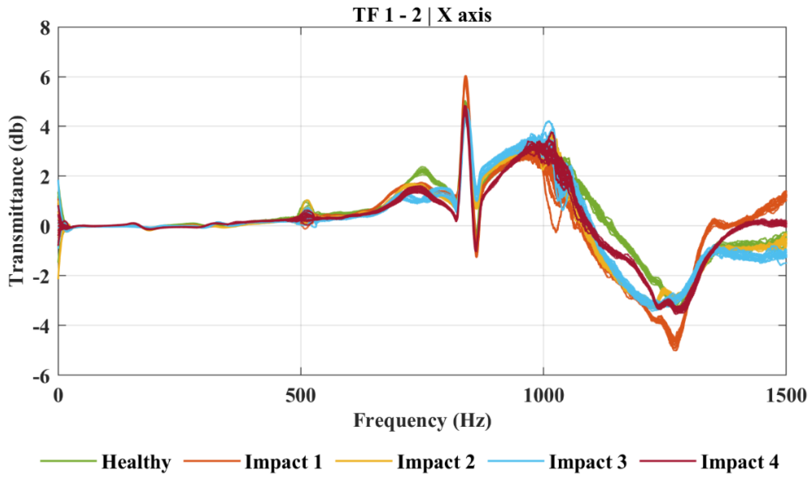
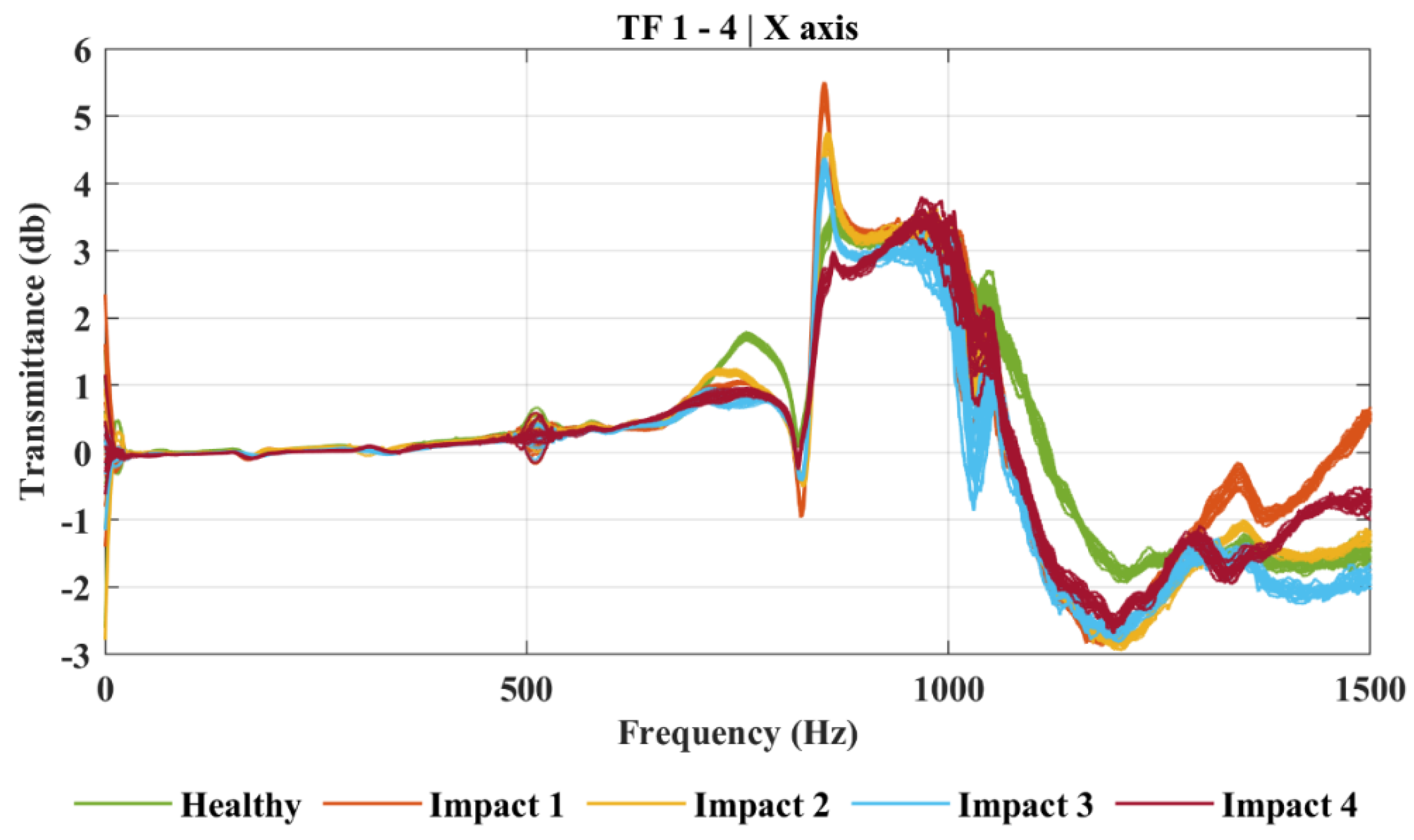
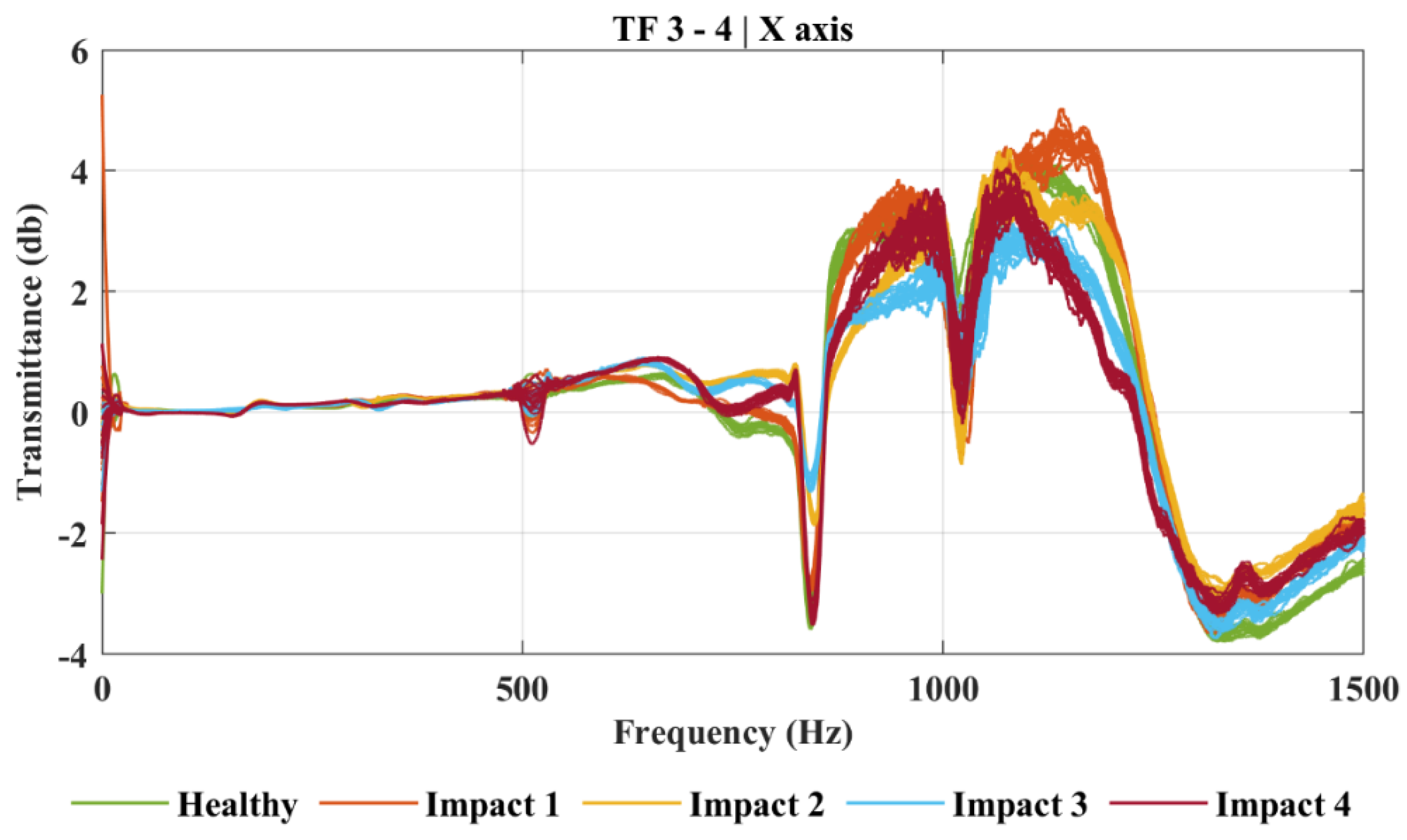
The estimation of the PSD for accelerometers A1 and A2 are presented Figure 5. It is noticeable that on most parts of the PSD curve, the damaged cases are indistinguishable. Even when the differences can be seen, the impact cases cannot be separated with great confidence. Conversely, in Figure 6, Figure 7 and Figure 8 with the TF curves between some of the accelerometers, the damage is distinguishable.

3.2. Clustering

The CFRP tank is generally a simple structure, as it does not contain moving parts and has simple geometry. The inspections of structural integrity, on the other hand, could be of great importance, as false estimation could lead to serious accidents due to the high internal pressure. During an inspection, a simple but effective method to estimate the tank’s status can be a valuable tool.
Clustering methods can be a valuable choice, but, as will be presented, caution must be taken in the selection of methods and tools.
The algorithms presented in Section 2 require an input of the clusters that will be created. In the context of damage detection, the first option is to separate the tanks’ states into two types: healthy and damaged. The second stage should be to create several groups with similar damaged states. An estimation could be made depending on the available database with experimental measurements. While the estimation of the number of clusters is not always possible as the inspection database enlarges, a solid methodology should be able to perform in both scenarios. For this reason, all options were tested using two clusters and the actual number of the tank’s states—five.
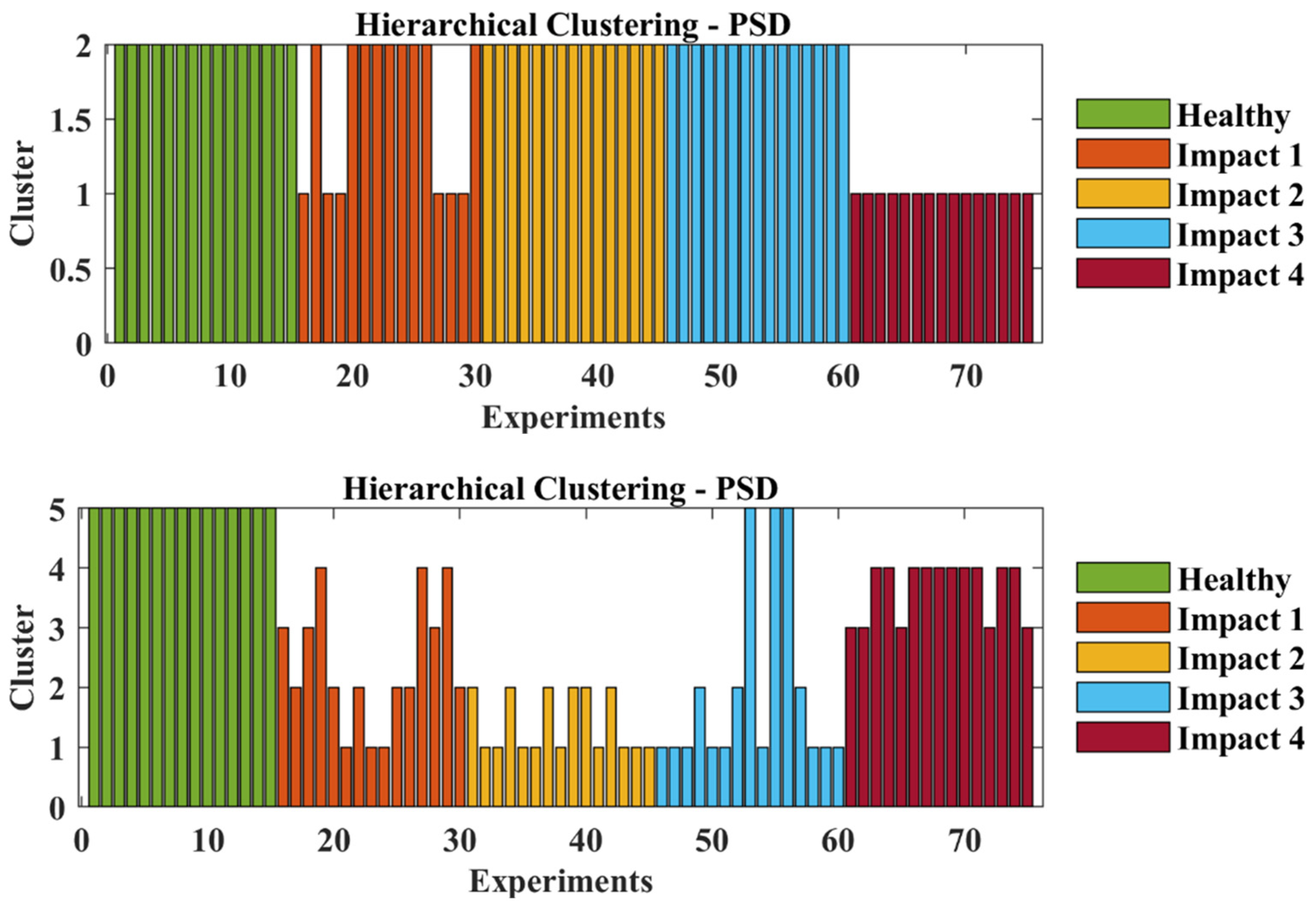
The first analysis uses PSD and hierarchical clustering Figure 9 presents the clusters (Y-axis) along with every experimental measurement (X-axis). The color of the bars represents the state of the tank during the experimental test. The numbers corresponding to the clusters do not represent any order or score. Either with two or with five clusters, this combination cannot perform, as several experiments have been grouped with different impact cases.
The combination of spectral clustering with the PSD is presented in Figure 10. It can successfully distinguish the damaged tanks from the healthy tanks when it is given two clusters. On the other hand, in the same Figure 10, with an input of five clusters, the damaged states cannot be separated properly.
Recalling the PSD curves that were presented in Figure 5, it was expected that it would not be an easy task to distinguish the cases, as the differences were small and sometimes hardly noticeable.
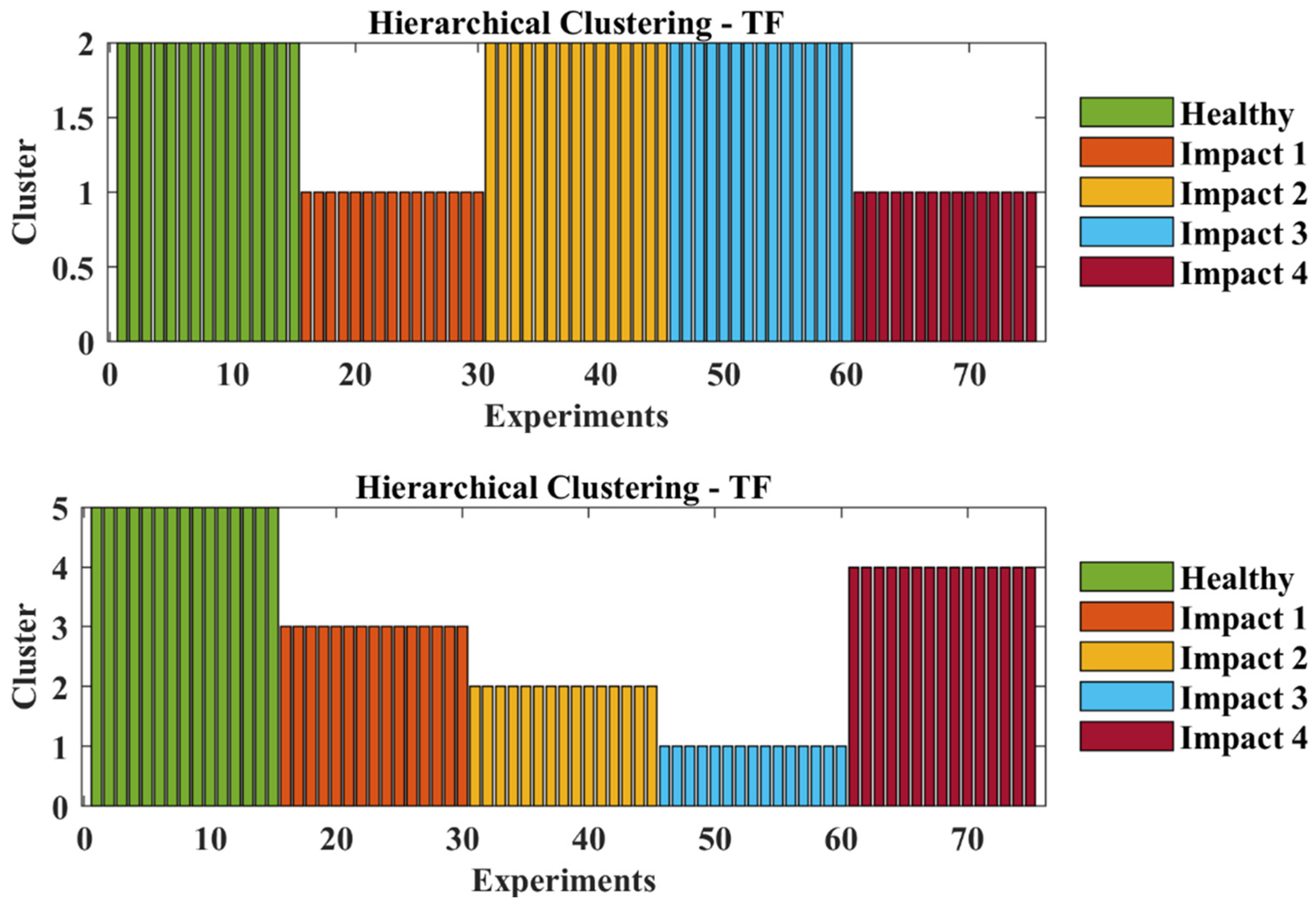
Continuing the application with the transmittance functions, Figure 11 presents the application of the hierarchical clustering algorithms. The first case, using an input cluster number of two, returns false results, as the impact cases 2 and 3 are grouped along with those in a healthy state. On the other hand, with a requested cluster of five, the experiments are grouped correctly. It must be noted again that the cluster identification number does not represent any order between the clusters, nor a score.
Following on from the last cases, the combination of the spectral clustering algorithm with the transmittance functions is presented in Figure 12. This combination achieved the correct results with both two and five requested clusters. When using two requested clusters, the healthy case exists within a different cluster from all of the damaged cases. Furthermore, with five requested clusters, all of the states, including the healthy and the impact cases, are only grouped in the same states of the tank.
It must be noted that after reviewing all of the combinations presented, the transmittance function seems to be a promising response-only metric for SHM. In Table 3, the final summary of the comparison is included. The difference between the PSD and TF is clear. The transmittance function is prone to material changes and highlights the differences. Because it is a relative measure between two acceleration signals, the TF is not dependent on the input excitation. Thus, it simplifies the testing procedure, where in this case, multiple tests on different identical tanks must be executed. Regarding the clustering algorithm, spectral clustering has provided more accurate and clear results and, together with the use of TF, it can be applied safely for inspection.
The proposed methodology has been validated on the examined structure, where the damage cases can be clustered successfully. It must be noted that all damage detection procedures have limitations. The existing procedure involved a certain minimum impact level of 10 joules. When applying the methodology, this lower damage limit could be a subject of further research, as the structure could have different characteristics. In an industrial environment, the amount of collected data could include a vast range of damaged cases, but may also include tanks in healthy states after production. As this amount is growing, the lower limit of the damage can be defined with better confidence.
The currently available data have been clustered successfully using the spectral-TF combination. The accuracy can be increased as the available data grow. Furthermore, as presented, no false healthy states were indicated with this level of damage. The level of uncertainty can only be defined with more available data from different damage levels and locations.
The spectral-TF procedure could also be used in conjunction with more complex algorithms in order to improve the procedure. One case could be to cluster a large amount of data into similar categories and use this information to train classification machine learning algorithms.

4. Conclusions

In this paper, a response-only approach was presented that utilized clustering algorithms and vibration measurements. Two well-established algorithms were compared for their ability to recognize the different states of a CFRP Type V tank. Furthermore, two response metrics were compared for their ability to provide the necessary information. The combination of spectral clustering algorithms and the transmittance function was shown to be most efficient, as it was able to distinguish between the different states of the tank in all cases.
The primary goal lies in the use of response-only metrics for vibration-based damage detection in the context of the inspection of many identical structures. A specific selection must be made on all parts to successfully identify a damaged state, as not all clustering algorithms and metrics can be successfully applied. The presented approach was tested on a relatively simple structure. Complex structures with multiple parts and joints could require prior testing to ascertain whether more complex algorithms are needed. Nevertheless, using the presented combination within regular inspections to clarify the state of tanks is feasible. Furthermore, during regular inspections, the available database of experimental measurements would grow, meaning that it could provide answers to different types and magnitudes of damage. In the context of this work, attention has been given to the impact damage that could occur on a CFRP tank. During transportation, installation, and usage of these high-pressure tanks there is a high possibility for something to hit the walls of the tank. To distinguish between the two states—healthy and damaged—the required data do not have to include exhaustive data sets of damaged cases. Lastly, the required experimental procedure is relatively simple and fast to implement.
The study reported in this paper demonstrates a good potential for the proposed approach for detecting damage in CFRP tanks. However, it should be noted that in order to implement the methodology for damage detection in the production line, additional work and refinement might be needed to increase the accuracy of the method and reduce possible false detections. One such example would be to continuously acquire new datasets of experimental measurements of tanks in healthy and damaged states in order to improve the accuracy.

Author Contributions

Conceptualization, I.Z. and D.G.; methodology, I.Z. and D.G.; software, I.Z.; validation, I.Z. and D.G.; formal analysis, I.Z. and D.G.; investigation, I.Z.; resources, D.G.; data curation, D.G.; writing—original draft preparation, I.Z.; writing—review and editing, D.G.; visualization, I.Z. and D.G.; supervision, D.G.; project administration, D.G.; funding acquisition, D.G. All authors have read and agreed to the published version of the manuscript.

Funding

This research was co-financed by the European Regional Development Fund of the European Union and Greek national funds through the Operational Program Competitiveness, Entrepreneurship, and Innovation, under the call RESEARCH—CREATE—INNOVATE (project code: T1EDK:05393).

Institutional Review Board Statement

Not applicable.

Informed Consent Statement

Not applicable.

Data Availability Statement

Data set available on request to corresponding authors.

Conflicts of Interest

The authors declare no conflict of interest.

References

  1. Das, S.; Warren, J.; West, D.; Schexnayder, S.M. Global Carbon Fiber Composites Supply Chain Competitiveness Analysis; Clean Energy Manufacturing Analysis Center: Golden, CO, USA, 2016. [Google Scholar]
  2. Yamashita, A.; Kondo, M.; Goto, S.; Ogami, N. Development of High-Pressure Hydrogen Storage System for the Toyota “Mirai”; SAE Technical Paper; SAE International: Detroit, MI, USA, 2015. [Google Scholar] [CrossRef]
  3. Berro Ramirez, J.P.; Halm, D.; Grandidier, J.C.; Villalonga, S.; Nony, F. 700 bar type IV high pressure hydrogen storage vessel burst—Simulation and experimental validation. Int. J. Hydrogen Energy 2015, 40, 13183–13192. [Google Scholar] [CrossRef]
  4. Robinson, M.; Stolzfus, J.; Owens, T. Composite material compatibility with liquid and gaseous oxygen. In Proceedings of the 19th AIAA Applied Aerodynamics Conference, Anaheim, CA, USA, 11–14 June 2001; American Institute of Aeronautics and Astronautics: Reston, VA, USA, 2001. [Google Scholar]
  5. Richardson, M.O.W.; Wisheart, M.J. Review of low-velocity impact properties of composite materials. Compos. Part A Appl. Sci. Manuf. 1996, 27, 1123–1131. [Google Scholar] [CrossRef]
  6. Meola, C.; Carlomagno, G.M. Non-destructive evaluation (NDE) of aerospace composites: Detecting impact damage. In Non-Destructive Evaluation (NDE) of Polymer Matrix Composites; Elsevier: Cambridge, UK, 2013; pp. 367–396. [Google Scholar]
  7. Bulletti, A.; Giannelli, P.; Calzolai, M.; Capineri, L. An Integrated Acousto/Ultrasonic Structural Health Monitoring System for Composite Pressure Vessels. IEEE Trans. Ultrason. Ferroelectr. Freq. Control 2016, 63, 864–873. [Google Scholar] [CrossRef] [PubMed]
  8. Huang, J.Q. Non-destructive evaluation (NDE) of composites: Acoustic emission (AE). In Non-Destructive Evaluation (NDE) of Polymer Matrix Composites; Elsevier: Cambridge, UK, 2013; pp. 12–32. [Google Scholar]
  9. Wong, B.S. Non-destructive evaluation (NDE) of composites: Detecting delamination defects using mechanical impedance, ultrasonic and infrared thermographic techniques. In Non-Destructive Evaluation (NDE) of Polymer Matrix Composites; Elsevier: Cambridge, UK, 2013; pp. 279–308. [Google Scholar]
  10. Heuer, H.; Schulze, M.H.; Meyendorf, N. Non-destructive evaluation (NDE) of composites: Eddy current techniques. In Non-Destructive Evaluation (NDE) of Polymer Matrix Composites; Elsevier: Cambridge, UK, 2013; pp. 33–55. [Google Scholar]
  11. Das, S.; Saha, P.; Patro, S.K. Vibration-based damage detection techniques used for health monitoring of structures: A review. J. Civ. Struct. Health Monit. 2016, 6, 477–507. [Google Scholar] [CrossRef]
  12. Zou, Y.; Tong, L.; Steven, G.P. Vibration-based model-dependent damage (delamination) identification and health monitoring for composite structures—A review. J. Sound Vib. 2000, 230, 357–378. [Google Scholar] [CrossRef]
  13. Gomes, G.F.; Mendez, Y.A.D.; da Silva Lopes Alexandrino, P.; da Cunha, S.S.; Ancelotti, A.C. A Review of Vibration Based Inverse Methods for Damage Detection and Identification in Mechanical Structures Using Optimization Algorithms and ANN. Arch. Comput. Methods Eng. 2019, 26, 883–897. [Google Scholar] [CrossRef]
  14. Gomes, G.F.; Mendéz, Y.A.D.; da Cunha, S.S.; Ancelotti, A.C. A numerical–experimental study for structural damage detection in CFRP plates using remote vibration measurements. J. Civ. Struct. Health Monit. 2018, 8, 33–47. [Google Scholar] [CrossRef]
  15. Zacharakis, I.; Arailopoulos, A.; Markogiannaki, O.; Giagopoulos, D. Damage detection in composite carbon fiber tubes based on experimental measurements and finite element model updating techniques. In Proceedings of the 7th International Conference on Computational Methods in Structural Dynamics and Earthquake Engineering (COMPDYN 2015), Crete, Greece, 24–26 June 2019; Institute of Structural Analysis and Antiseismic Research School of Civil Engineering National Technical University of Athens (NTUA): Athens, Greece, 2019; Volume 2, pp. 2959–2970. [Google Scholar]
  16. Zacharakis, I.; Arailopoulos, A.; Markogiannaki, O.; Giagopoulos, D. Vibration based structural health monitoring of composite carbon fiber structural systems. In Proceedings of the 3rd International Conference on Uncertainty Quantification in Computational Sciences and Engineering, Uncecomp 2019, Crete, Greece, 24–26 June 2019. [Google Scholar]
  17. Zacharakis, I.; Giagopoulos, D.; Zyganitidis, I.; Arailopoulos, A.; Markogiannaki, O. Modeling of cfrp structures using model updating techniques and experimental measurements. In Proceedings of the International Conference on Structural Dynamic, EURODYN, Athens, Greece, 23–26 November 2020; Volume 1, pp. 536–550. [Google Scholar]
  18. Mechbal, N.; Uribe, J.S.; Rébillat, M. A probabilistic multi-class classifier for structural health monitoring. Mech. Syst. Signal Process. 2015, 60–61, 106–123. [Google Scholar] [CrossRef] [Green Version]
  19. Bull, L.A.; Worden, K.; Dervilis, N. Towards semi-supervised and probabilistic classification in structural health monitoring. Mech. Syst. Signal Process. 2020, 140, 106653. [Google Scholar] [CrossRef]
  20. Santos, A.; Figueiredo, E.; Silva, M.F.M.; Sales, C.S.; Costa, J.C.W.A. Machine learning algorithms for damage detection: Kernel-based approaches. J. Sound Vib. 2016, 363, 584–599. [Google Scholar] [CrossRef]
  21. Hou, R.; Xia, Y. Review on the new development of vibration-based damage identification for civil engineering structures: 2010–2019. J. Sound Vib. 2021, 491, 115741. [Google Scholar] [CrossRef]
  22. Seventekidis, P.; Giagopoulos, D.; Arailopoulos, A.; Markogiannaki, O. Structural Health Monitoring using deep learning with optimal finite element model generated data. Mech. Syst. Signal Process. 2020, 145, 106972. [Google Scholar] [CrossRef]
  23. Seventekidis, P.; Giagopoulos, D. A combined finite element and hierarchical Deep learning approach for structural health monitoring: Test on a pin-joint composite truss structure. Mech. Syst. Signal Process. 2021, 157, 107735. [Google Scholar] [CrossRef]
  24. Andriosopoulou, G.; Mastakouris, A.; Vamvoudakis-Stefanou, K.; Fassois, S. Random Vibration Based Robust Damage Detection for a Composite Aerostructure Under Assembly-Induced Uncertainty. In Proceedings of the 13th International Conference on Damage Assessment of Structures, Porto, Portugal, 9–10 July 2019; Lecture Notes in Mechanical Engineering. Springer: Singapore, 2020; pp. 775–787, ISBN 9789811383304. [Google Scholar]
  25. Pedram, M.; Esfandiari, A.; Khedmati, M.R. Damage detection by a FE model updating method using power spectral density: Numerical and experimental investigation. J. Sound Vib. 2017, 397, 51–76. [Google Scholar] [CrossRef]
  26. Zhang, H.; Schulz, M.J.; Naser, A.; Ferguson, F.; Pai, P.F. Structural health monitoring using transmittance functions. Mech. Syst. Signal Process. 1999, 13, 765–787. [Google Scholar] [CrossRef]
  27. Poulimenos, A.G.; Sakellariou, J.S. A transmittance-based methodology for damage detection under uncertainty: An application to a set of composite beams with manufacturing variability subject to impact damage and varying operating conditions. Struct. Health Monit. 2019, 18, 318–333. [Google Scholar] [CrossRef]
  28. Langone, R.; Reynders, E.; Mehrkanoon, S.; Suykens, J.A.K. Automated structural health monitoring based on adaptive kernel spectral clustering. Mech. Syst. Signal Process. 2017, 90, 64–78. [Google Scholar] [CrossRef] [Green Version]
  29. Zhou, Y.-L.; Maia, N.M.M.; Sampaio, R.P.C.; Wahab, M.A. Structural damage detection using transmissibility together with hierarchical clustering analysis and similarity measure. Struct. Health Monit. 2017, 16, 711–731. [Google Scholar] [CrossRef]
  30. Nielsen, F. Introduction to HPC with MPI for Data Science; Undergraduate Topics in Computer Science; Springer International Publishing: Cham, Switzerland, 2016; ISBN 978-3-319-21902-8. [Google Scholar]
  31. Jain, A.K.; Murty, M.N.; Flynn, P.J. Data clustering: A review. ACM Comput. Surv. 1999, 31, 264–323. [Google Scholar] [CrossRef]
  32. Aldenderfer, M.; Blashfield, R. Cluster Analysis; SAGE Publications, Inc.: Thousand Oaks, CA, USA, 1984; ISBN 9780803923768. [Google Scholar]
  33. Ng, A.Y.; Jordan, M.I.; Weiss, Y. On Spectral Clustering: Analysis and an Algorithm. In Proceedings of the 14th International Conference on Neural Information Processing Systems: Natural and Synthetic, Vancouver, BC, Canada, 3–8 December 2001; MIT Press: Cambridge, MA, USA, 2001; pp. 849–856. [Google Scholar]
  34. Meilua, M.; Shi, J. A Random Walks View of Spectral Segmentation. In Proceedings of the Eighth International Workshop on Artificial Intelligence and Statistics, Key West, FL, USA, 4–7 January 2001; Richardson, T.S., Jaakkola, T.S., Eds.; 2001; Volume R3, pp. 203–208. [Google Scholar]
  35. Shi, J.; Malik, J. Normalized cuts and image segmentation. IEEE Trans. Pattern Anal. Mach. Intell. 2000, 22, 888–905. [Google Scholar] [CrossRef] [Green Version]
  36. Von Luxburg, U. A tutorial on spectral clustering. Stat. Comput. 2007, 17, 395–416. [Google Scholar] [CrossRef]
  37. Pedregosa, F.; Varoquaux, G.; Gramfort, A.; Michel, V.; Thirion, B.; Grisel, O.; Blondel, M.; Prettenhofer, P.; Weiss, R.; Dubourg, V.; et al. Scikit-learn: Machine Learning in {P}ython. J. Mach. Learn. Res. 2011, 12, 2825–2830. [Google Scholar]
  38. The MathWorks Inc. MATLAB 2020. Available online: https://www.mathworks.com/ (accessed on 8 December 2021).
  39. Roux, M. A Comparative Study of Divisive and Agglomerative Hierarchical Clustering Algorithms. J. Classif. 2018, 35, 345–366. [Google Scholar] [CrossRef] [Green Version]
  40. Maia, N.M.M.; Almeida, R.A.B.; Urgueira, A.P.V.; Sampaio, R.P.C. Damage detection and quantification using transmissibility. Mech. Syst. Signal Process. 2011, 25, 2475–2483. [Google Scholar] [CrossRef]
  41. Chesné, S.; Deraemaeker, A. Damage localization using transmissibility functions: A critical review. Mech. Syst. Signal Process. 2013, 38, 569–584. [Google Scholar] [CrossRef] [Green Version]
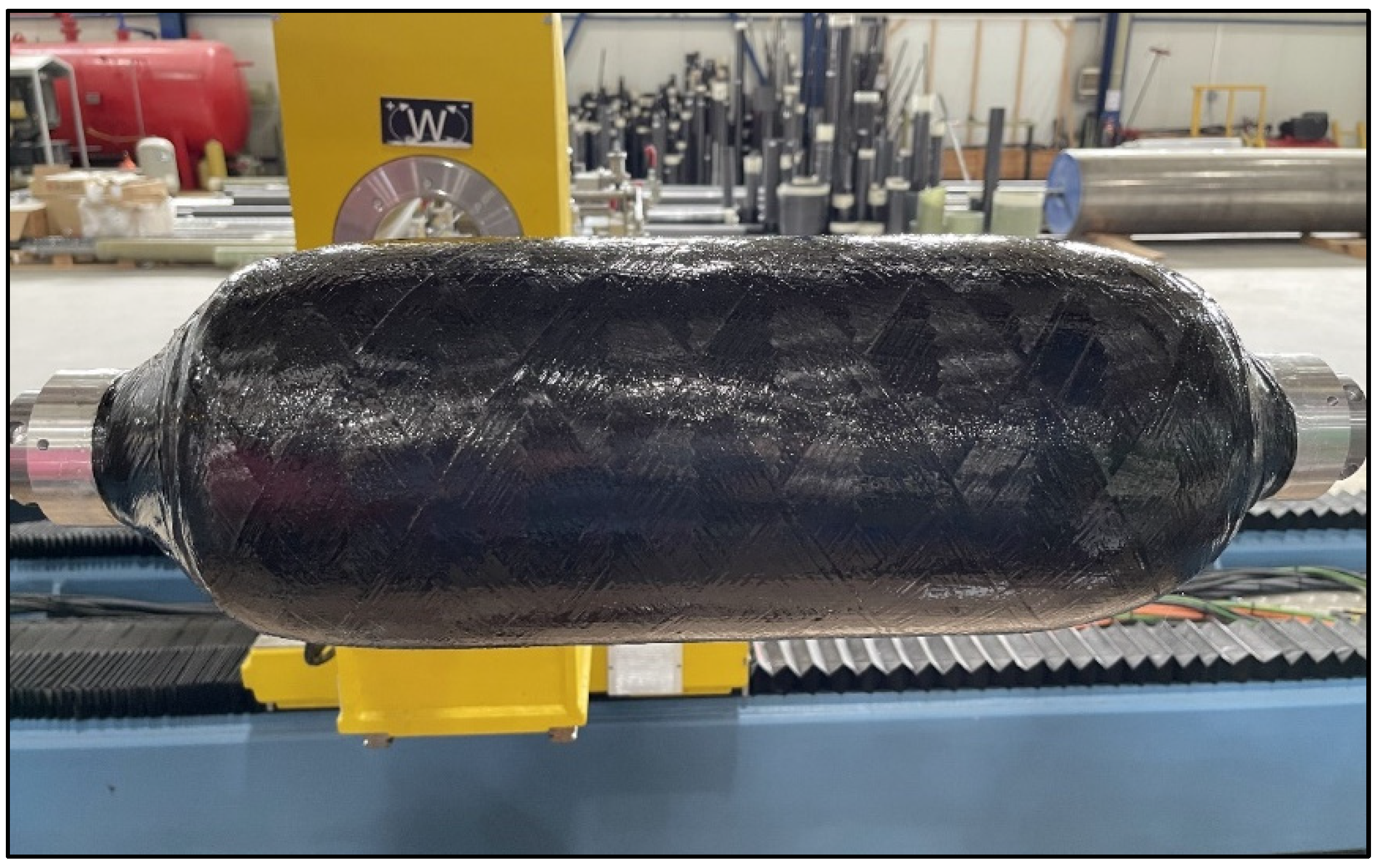
Figure 1. CFRP tank during the filament winding.
Applmech 02 00061 g001
Figure 2. Experimental setup of the CFRP tank (left). Radial placement of accelerometers (right).
Applmech 02 00061 g002
Figure 3. Indicative eigenmodes of the FE model in the range of 0 to 1500 Hz.
Applmech 02 00061 g003
Figure 4. Impact setup on the CFRP tank.
Applmech 02 00061 g004
Figure 5. Power spectral density (PSD) of accelerometers A1 and A2.
Applmech 02 00061 g005
Figure 6. Transmittance functions (TF) on X-axis between accelerometer A1 and accelerometer A2.
Applmech 02 00061 g006
Figure 7. Transmittance functions (TF) on X-axis between accelerometer A1 and accelerometer A4.
Applmech 02 00061 g007
Figure 8. Transmittance functions (TF) on X-axis between accelerometer A3 and accelerometer A4.
Applmech 02 00061 g008
Figure 9. Hierarchical clustering using PSD. Input cluster = 2 (up), input cluster = 5 (down).
Applmech 02 00061 g009
Figure 10. Spectral clustering using PSD. Input cluster = 2 (up), input cluster = 5 (down).
Applmech 02 00061 g010
Figure 11. Hierarchical clustering using TF. Input cluster = 2 (up), input cluster = 5 (down).
Applmech 02 00061 g011
Figure 12. Spectral clustering using TF. Input cluster = 2 (up), input cluster = 5 (down).
Applmech 02 00061 g012
Table 1. Accelerometer location.
AccelerometerHeight (mm)Angle (Degrees)
A12400
A2480135
A3300180
A4420270
Table 2. Impact experiments.
ExperimentImpact Energy (Joules)Vibration Experiments
Healthy-15
Impact 11015
Impact 21015
Impact 31015
Impact 41015
Table 3. Results summary.
MeasureClustering MethodCluster InputResult
Power Spectral Density (PSD)Hierarchical2False
5False
Spectral2Correct
5False
Transmittance Function (TF) Hierarchical2False
5Correct
Spectral2Correct
5Correct
Publisher’s Note: MDPI stays neutral with regard to jurisdictional claims in published maps and institutional affiliations.