Abstract
In engineering, metaheuristic algorithms have been used to solve complex optimization problems. This paper investigates and compares various algorithms. On one hand, the study seeks to ascertain the advantages and disadvantages of the newly presented heuristic techniques. The efficiency of the algorithms is highly dependent on the nature of the problem. The ability to change the complexity of the problem and the knowledge of global optimal locations are two advantages of using synthetic test functions for algorithm benchmarking. On the other hand, real-world design issues may frequently give more meaningful information into the effectiveness of optimization strategies. A new synthetic test function generator has been built to examine various optimization techniques. The objective function noisiness increased significantly with different transformations (Euclidean distance-based weighting, Gaussian weighting and Gabor-like weighting), while the positions of the optima remained the same. The test functions were created to assess and compare the performance of the algorithms in preparation for further development. The ideal proportions of the primary girder of an overhead crane have also been discovered. By evaluating the performance of fifteen metaheuristic algorithms, the optimum solution to thirteen mathematical optimization techniques, as well as the box-girder design, is identified. Some conclusions were drawn about the efficiency of the different optimization techniques at the test function and the transformed noisy functions. The overhead travelling crane girder design shows the real-life application.
1. Introduction
It is tough to gauge which optimization algorithm is the most successful. A variety of novel evolutionary methods have recently surfaced. The performance of a novel metaheuristic algorithm should be objectively compared to that of previous algorithms when it is described. A wide range of test routines is provided for creating benchmarks. Some are entirely new [1]. When available resources are scarce, the optimum approach is utilized to discover the best solution to a problem. Despite the rapid advancement of computer science, most optimization issues cannot be addressed by examining all possible options. NP-hard tasks, such as the Traveling salesman problem (also known as TSP), may have a large search area that must be thoroughly explored in exponential computing time. Metaheuristic algorithms can find approximate answers even when the search space is excessively vast. The efficiency of fifteen optimization methods in identifying global minima of diverse continuous mathematical test functions is compared in this paper. Mathematical function optimization is essential because it can be used to solve most real-world optimization issues. In the literature there exist numerous mathematical test functions. A software solution that utilizes a unique method for building bespoke test functions has also been created. In this paper, first those test functions are introduced which are used in the evaluation process. A new synthetic test function generator has been built to examine various optimization techniques. The function transformations to make the objective functions noisier are described using Euclidean distance-based weighting, Gaussian weighting and Gabor-like weighting. At the same time, the positions of the optima remain the same. The crane girder optimization shows the applicability of the optimizers for a real-life problem. The efficiency is different, information which helps users to select the proper algorithm.
2. Materials and Methods—Benchmark Problems
Several mathematical test functions may be found in the literature, such as in the paper of Mologa and Smutnicki [2]. The number of variables and the number and distribution of local extremes affects the complexity of test functions. Continuous test functions with two variables were investigated because such issues may be represented as 3D surfaces. Table 1 lists the ten test functions that were utilized in alphabetical order. The centre of Ackley’s function is a massive valley, with a somewhat level outside part. Metaheuristic algorithms are easily captured by one of the local optima of this frequently used multimodal test function. The problem scenario is as follows: First we check the efficiency of the algorithms using the test functions. Then, using function transformations, we make the objective functions noisier to make the problem-solving more difficult. After that, we use the optimizers for a real-life problem.

Table 1.
The most crucial information about benchmark problems (all functions are minimized, n is the number of design variables).
The benchmark problem of DeJong’s function is unimodal, simple, and convex. The Drop-Wave function is very complicated when an object is dropped into a liquid surface, increasing ripples. Similar to De Jong’s function, Easom’s function is unimodal, but it is more challenging since the global optimum is small concerning the search space. Griewangk’s function has a rough surface with numerous equally scattered local optima, similar to De Jong’s function. Matyas’ function is a plate-shaped issue with no local extremes and just one global extreme, which is very simple to locate.
Convergence to the global optimum is challenging, making it an excellent benchmark for assessing the accuracy and pace of convergence of search algorithms. The egg holder, or Rastrigin’s function, is a widely used, highly multimodal issue with regularly distributed local extremes. In Rosenbrock’s valley, which is unimodal, the global minimum may be located in a small, parabolic valley. Schaffer’s test function is quite noisy, having many local optima that are very close to each other. Finally, the Three-hump camelback resembles the Rosenbrock Valley in look, but with two local extremes.
The minimum and maximum values of the variables are the Searchspace (min) and (max) in the pseudocodes of the different algorithms.
3. Composition of Test Functions
Liang et al. [3] proposed a novel theoretical method for deriving more complex test functions from simpler ones. The idea behind creating a composition of functions is that the weighted sum of a few simple basic functions with a known optimum may quickly provide severe test challenges for heuristic algorithms. We may create a broad range of test issues using the composition of functions since the kind and quantity of essential functions can be dynamically defined. Barcsák and Jármai [4] have developed a realistic framework that builds on the previous concept. A software solution has been created that uses the practical base to efficiently create customized, arbitrarily complicated test problems.
3.1. Theoretical Method
In order to create arbitrarily elaborate and sophisticated test functions, the method requires a large number of input parameters:
- [Xmin, Xmax]D: search range of the complex function;
- : number of dimensions;
- fi(θ): list of basic functions, where θ ∈ RD;
- [xmin, xmax]D: search range of the basic functions;
- oi: the global optimum position for the i-th basic function;
- bias: a vector that identifies the global best solution. This allows the user to change the basic functions’ optimal values. A vector to define the global optimum.
The values of the global optimum points of the basic function must be actually unchanged in order to specify the position of global and local optima. To accomplish this, the fundamental functions must be evaluated outside of the search range specified. As a result, the global optimal placements of the core functions must be independent of the search range. The complicated test functions can be determined using the following equations:
where and the weighting function wi guarantees that the preset ideal placements and values are maintained; nevertheless, the first function has the most significant weighting number, while the others have equal or smaller weighting numbers. The higher the weighting coefficient, the closer the solution comes to locating the global optimal location (oi) of a basic function. The weighting coefficients of the other fundamental function(s) are decreased at the same time. Weighting functions were used in three different ways.
3.1.1. Euclidean Distance-Based Weighting
The first weighting function uses the Euclidean distance between the provided point of the complex function (. ) and the optimum locations () of the basic function.
The following are the normalized distances:
where means the sum of the weightings
If , and is the number of basic functions:
3.1.2. Gaussian Weighting
Using Gaussian functions to derive weighting factors can result in smoother edges.
3.1.3. Gabor Weighting
If the weighting function introduces noise, more difficult optimization issues may arise. It is critical, however, not to stray from the original optimal settings. The weighting function should return values between 0 and 1, with its global maxima located at the global optimum of the complicated function.
where is the k-th element of the . vector, is the parameter for noise, and is the range of convergence. Increasing the parameter, more noise will occur. If , and is the number of basic functions:
3.2. Practical Example
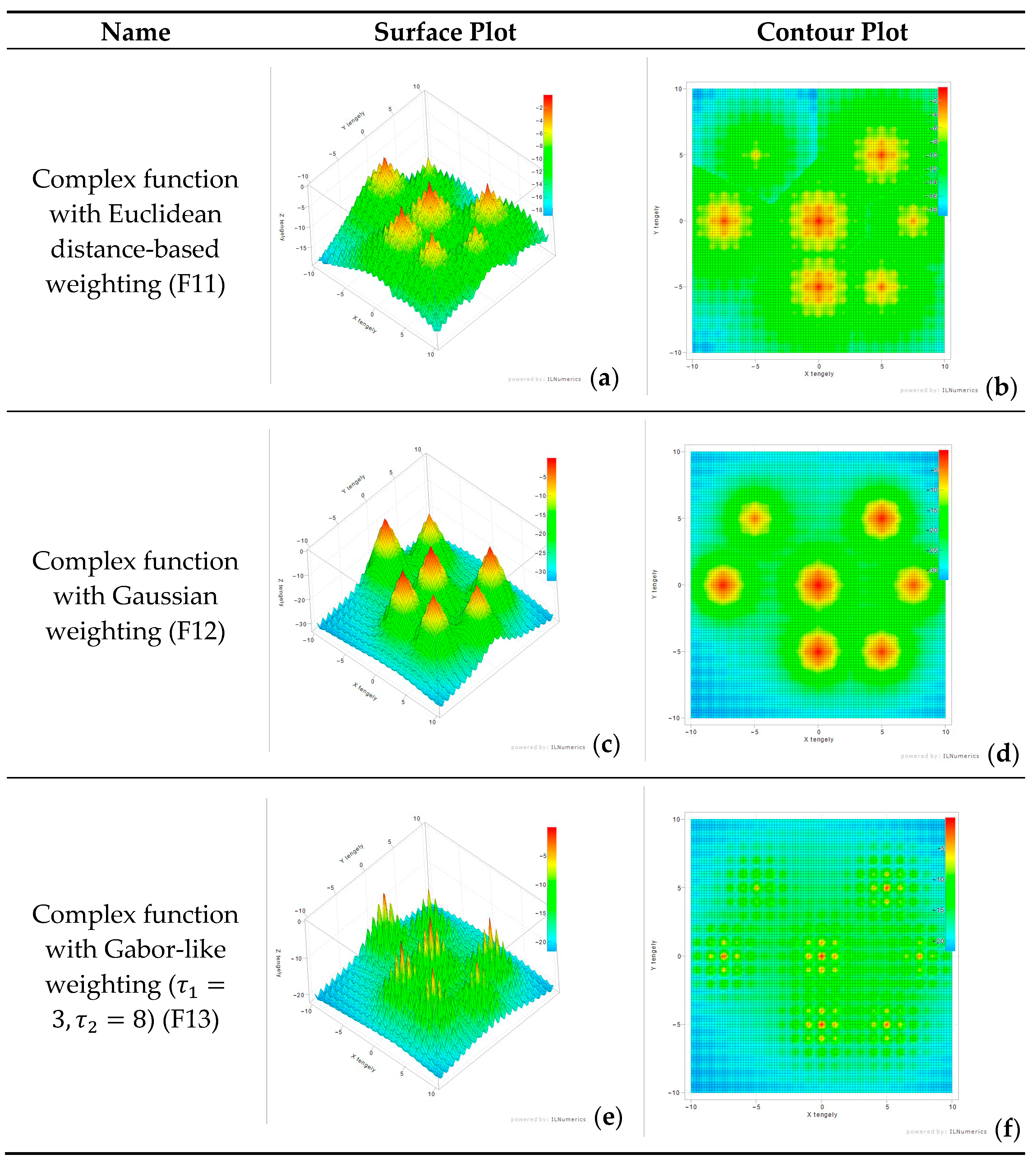
A complicated test function was created to show the strategy and increase the number of benchmark issues utilized in this research (Figure 1). The parameters for input are as follows:
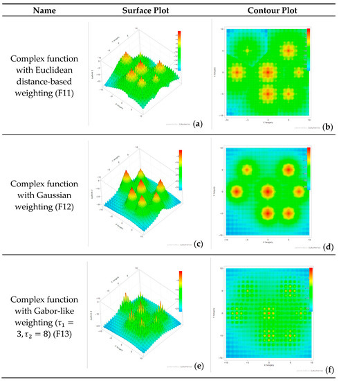
Figure 1.
Surface and contour plots of complex benchmark problems. (a) Surface plot of complex function with Euclidean distance-based weighting; (b) Contour plot of complex function with Euclidean distance-based weighting; (c) Surface plot of complex function with Gaussian weighting; (d) Contour plot of complex function with Gaussian weighting; (e) Complex function with Gabor-like weighting (τ1 = 3, τ2 = 8); (f) Contour plot of Complex function with Gabor-like weighting (τ1 = 3, τ2 = 8).
- : The search area of the complicated function is
- : dimension count is 2
- : 7 basic functions have been used; all of them are Ackley functions (F1).
- There is no need to define the search range of the basic functions because the optimal locations have been shifted.
- : the coordinates for optima of the basic functions: [7.5; 5; 5; 0; −7.5; −5; 0]
- : the coordinates for optima of the basic functions: [0; 5; −5; −5; 0; 5; 0]
- Bias: a vector to shift the basic functions: [3; 1; 2; 0.5; 1; 4.5; 0]
3.3. Novel Software Solution to Easily Generate Complex Test Functions
Using the framework described above, a software solution has been built that makes it simple to create customized arbitrarily severe test tasks. The application operated on the NET Framework and was developed entirely in C#. The most pleasing aspect of the software is the automated source code creation. The machine generates the C# source code for the complicated function while the user builds it in a visual editor. As a consequence, the newly created optimization issue may be used right away.
4. Main Characteristics of Metaheuristic Algorithms
As previously stated, metaheuristic algorithms benefit from identifying approximation answers even when the search space is incredibly vast. However, obtaining the global optimum cannot be guaranteed because they do not consider all alternative options. Metaheuristic algorithms improve computer performance, but accuracy may suffer as a result.
A suitable metaheuristic algorithm must be used to maintain the balance between local and global searches. On the one hand, it must do a thorough investigation of the whole search region; on the other hand, it must conduct a quick search around the current best places. In other words, instead of wasting time in low-quality areas, the aim is to discover regions with high-quality solutions quickly. The majority of heuristic algorithms exhibit stochastic behaviour. Even if the final responses differ somewhat they should, in principle, converge to the optimum solution for the particular issue.
However, due to the stochastic nature of metaheuristic algorithms, the approach used to arrive at a solution is always a bit different. Many nature-inspired metaheuristic algorithms have emerged based on the behavior of biological and physical systems. Fifteen optimization techniques were investigated, including evolutionary (Cultural Algorithm, Differential Evolution, Memetic Algorithm), physical (Harmony Search, Simulated Annealing, Cross-Entropy Method), swarm intelligence (Bacterial Foraging, Bat Algorithm, Bees Algorithm, Cuckoo Search, Firefly, Particle Swarm and Multi-Swarm Optimization), swarm intelligence (Bacterial Foraging, Bat Algorithm, Bees Algorithm, Cuckoo Search, Firefly, Particle Swarm and Multi-Swarm Optimization) and other methods such as Nelder—Mead and Random Search.
Some of the innovative approaches that have been created are Virus optimization [1], Dynamic differential annealed optimization [5], Hybrid multi-objective optimization [6], or Big bang–big crunch algorithm [7], and Water evaporation optimization [8]. The performance of mixed metaheuristic algorithms can be improved [9]. Multi-objective evolutionary algorithms are necessary when there are several objective functions [10,11,12]. Brownlee describes various metaheuristic algorithms in his book [13].
Benchmarked Metaheuristic Algorithms
Liu and Passino [14] initially described and published the Bacterial Foraging Optimization Algorithm (BFOA) in 2002. It is a recently developed swarm intelligence search method. These techniques rely on the collective intelligence of a group of people who are all similar. In theory, a single organism may not be able to solve a problem on its own. However, if a group of individuals develops, the combined intellect of the group may be adequate to finish the task. The foraging and reproductive behavior of E. coli bacteria colonies provide the basis for Bacterial Foraging. The chemotaxis movement of the group is focused on obtaining vital nutrients (global optimum) while avoiding potentially hazardous surroundings (local optima).
Yang [15], a swarm intelligence metaheuristic method based on bat echolocation, published the Bat Algorithm (BATA) in 2010. Bats can find and identify prey (global optimum) and avoid obstacles using echolocation even in total darkness (local optima). Similar to sonar, bats produce a sound pulse and listen for the echo that returns from the surroundings. During the search, the frequency, volume, and rate of emission of the individual sound, which indicates the position of the prey, varies, alerting other bats. The loudness of the sound the bat makes decreases as it comes closer to the prey, but the rate at which it emits pulses rises. The Bat Algorithm combines the advantages of Particle Swarm Optimization and the Firefly Algorithm, two current swarm intelligence techniques.
The Bees Algorithm (BA) was published in 2005 by Pham et al. [16]. It was developed mainly to determine the global optimum of continuous mathematical functions. It falls within the swarm intelligence technique category. The Bees Algorithm was inspired by honey bee foraging activity, as the name suggests. Bee colonies send out scout bees to explore the surroundings and find nectar-rich spots (global or local optima). When the scout bees return to the hive, they inform the worker bees about the location and quality of food sources. The number of worker bees dispatched to each food source is influenced by these parameters. Scout bees are always on the hunt for appropriate locations, while worker bees inspect those that have already been found.
On the other hand, Scout bees are in charge of global search, whilst worker bees are in charge of local search. Both Ant Colony and Particle Swarm Optimization are equivalent approaches. Bees, on the other hand, have a hierarchy of their own. The Bees Algorithm may be used to tackle both continuous and combinatorial optimization problems.
In 1997, Rubinstein [17] introduced the Cross-Entropy Method (CEM), a probabilistic optimization method. The method gets its name from the Kullback—Leibler cross-entropy divergence, a similarity measure between two probability distributions. The Cross-Entropy Method is an adaptive significance estimate approach for rare-event probability in discrete event simulation systems. Optimization problems are classed as rare-event systems because the likelihood of discovering an optimal solution via a random search is a rare event probability. The approach modifies the random search sample distribution to make the improbable occurrence of finding the optimal solution more likely.
The Cuckoo Search (CS) Algorithm was created and published by Yang and Deb [18] in 2009. The algorithm was inspired by the brood parasitism of certain cuckoo species, which means they lay their eggs in the nests of other host species. If the host birds discover the foreign eggs are not their own, they can either reject them or leave the existing nest and create a new one somewhere else. The method randomly distributes a fixed number of nests over the search space. The cuckoos lay their eggs one at a time in a nest that they choose at random. A cuckoo egg symbolizes a unique solution, and each egg in a nest represents a solution. The algorithm aims to find a new, perhaps better solution (global optimum) to replace the faulty one (local optima). The members of the next generation will come from the best nests with the best eggs.
The Cultural Algorithm (CA) was created by Reynolds [19] and published in 1994. This evolutionary algorithm depicts the progression of cultural evolution for human society. The habits, beliefs, and values of an individual make up their culture. Culture may have a beneficial or detrimental impact on the environment due to feedback loops. This creates a knowledge base of both good and potentially harmful input about large areas of the environment (the global optimum) (local optima). Generations build and use this cultural knowledge base as circumstances change.
The Differential Evolution (DE) technique, developed by Storn and Price [20], was published in 1995 and was part of the field of evolutionary algorithms. Natural selection is the central tenet of Darwin’s Theory of Evolution, founded on natural selection. The method maintains a population of potential solutions throughout generations by recombination, assessment, and selection. Recombination generates a new viable solution based on the weighted difference between two randomly selected population members connected to a third population member.
Yang [21] developed and published the Firefly (FF) Technique, a multimodal optimization metaheuristic algorithm inspired by nature. The flashing behavior of fireflies to engage with other fireflies was the inspiration for the software. Bioluminescence, a biological process that causes flashing lights, may be utilized to attract both potential mates and prey. It can also be used as an early warning system. The speed with which the light flashes and the intensity with which it flashes are essential communication components. The flashing light can be linked to the goal function that has to be improved. As it comes closer to the proper solution, a firefly will produce more light. The less luminous fireflies will flock to the more dazzling ones. The attraction of a firefly is proportional to its brightness, which diminishes as the distance between them rises. The firefly will travel at random if there are no other glowing fireflies in the vicinity. The Firefly Algorithm is more adaptable to changes in attractiveness than other algorithms, such as Particle Swarm Optimization, and its visibility may be changed. To improve efficiency, the technique has undergone several substantial adjustments [22].
Harmony Search (HS) was released in 2001 by Geem et al. [23]. It was influenced by the improvisation of jazz musicians. When they begin a musical performance, they adjust their songs to the band, resulting in vocal harmony. When a phoney sound is heard, each group member modifies their behavior to improve their performance. The musicians regard harmony as a full possible answer, and they seek balance through minor changes and improvisation. The aesthetic appreciation of the audience for harmony represents the cost function. Similar to the Cultural Algorithm, the candidate solution components are either stochastically generated directly from the memory of high-quality solutions, changed from the memory of high-quality solutions, or allocated randomly.
In 1989, Moscato [24] invented the Memetic Algorithm (MA). The program mimics the generation of cultural information and its transmission from one person to another. The basic unit of cultural knowledge is the meme, which is derived from the biology word gene (an idea, a discovery, etc.). Universal Darwinism is the expansion of genes beyond biological systems to any system where discrete bits of information may be transmitted and subjected to evolutionary change. The objective of the algorithm is to conduct a population-based global search while individuals do local searches to locate appropriate locations. A balance between global and local search strategies is vital to guarantee that the algorithm does not become trapped in a local optimum while saving computing resources. A meme is a piece of information about the search that is passed down from generation to generation and has an evolutionary impact. Genetic and cultural evolution approaches are combined in the Memetic Algorithm.
The Nelder-Mead (NM) algorithm was called after Nelder and Mead [25], who introduced this metaheuristic approach in 1965. In the literature, the method is referred to as the Amoeba Method [26]. Nelder—Mead is a simplex search technique that employs a nonlinear optimization approach. The method produces a set of randomly generated candidate solutions, each with its unique fitness function value. Their fitness rates the options, and with each generation the algorithm tries to replace the poorest answer with a better one. The three options for the optimal solution are the reflected point, the extended point, and the contracted point. All of these locations are in a line, from the most inconvenient to the centroid. The centroid, with the exception of the worst point, is at the center of all points. If neither of the locations is better than the current worst solution, the amoeba moves all points halfway to the best point except the best location.
Particle Swarm Optimization (PSO), a swarm intelligence metaheuristic algorithm created by Eberhart and Kennedy [27], was first implemented in 1995. The foraging behavior of bird and fish swarms was the inspiration for the function of Particle Swarm. The particles of the swarm move throughout the search area, looking for places with a long history. The best-known position of each particle as well as of the swarm impact their new position. The mathematical techniques used by the movement determine the new particle velocity and position, guiding the swarm to the global optimum. In each generation, the process is repeated, with random impacts on particle mobility. On the development and application of PSO, several articles [28,29,30] have been published.
Multi-Swarm Optimization is a subset of Particle Swarm Optimization (PSO) (MSO). Instead of a single swarm, MSO uses a user-defined number of swarms to find the global optimum [31]. The technique is particularly effective for multimodal optimization problems involving a large number of local optima. Multi-Swarm Optimization [32] is a new approach for optimizing the global and local search balance.
As the name indicates, the Random Search (RS) algorithm is a basic random search method. It has an identical chance of landing in any place in the search space [33]. New solutions are always distinct from those that came before them. Random search provides a candidate solution building and assessment approach.
The Simulated Annealing (SA) approach was described and published by Kirkpatrick [34] in 1983. The functioning of the algorithm is based on a physical phenomenon. Certain materials develop beneficial characteristics when heated and subsequently cooled under controlled circumstances in metallurgy. During the process, the crystal structure of the material changes as the particles pick more advantageous locations. The metaheuristic algorithm, which seeks for better solutions to a given issue, mimics this process. Each algorithm result is a representation of the energy state of the system. The Metropolis-Hastings Monte Carlo method controls the acceptance of the new location. The sample acceptance criteria are tightened as the system cools, focusing on increasing mobility. The size of the neighbourhood used to generate candidate solutions might change over time or be impacted by temperature, beginning large and narrowing as the algorithm is run. A basic linear cooling regime is used with a high beginning temperature that is steadily lowered with each repetition. If the cooling phase is long enough, the system should always converge to the global optimum. The continuous version of the technique was created by Corana et al. [35]. It is currently being improved in order to improve its performance [36].
List of the tuning settings for the various techniques are shown in Table 2. Theses values are generally sufficient, but as the number of unknowns grows and the constraints become increasingly nonlinear, some changes are necessary.
Table 2.
List of the tuning settings for the various techniques *.
The internal parameters of each algorithm have been set from the literature and from our own experiences. There are newer techniques also available to improve the efficiency of the optimization, such as Arithmetic Optimization [37], the newly published Aquila Optimizer [38] and some new comparisons which were made [39].
5. Numerical Experiments
It is a time-consuming and challenging process to compare metaheuristic optimization approaches. Because the algorithms are stochastic, statistical techniques were used to produce relevant results. Each test function was subjected to 100 Monte Carlo searches by the metaheuristic algorithms. This implies that the computed 100 were chosen at random from a large pool of possibilities. The maximum number of iterations for each search was set at 500. It is clear that maximizing iteration number is not the best option to make good comparisons. However, we found that in most cases, the optimizers were close enough to the optima to be comparable. It was built in the same way as the other F1–F13 test functions.
5.1. Statistical Results
In the statistics tables, the performance of algorithms at various test functions is summarized (Table 3 and Table 4). The specified method(s) yielded the best results (shown in bold letters). Table 4 also shows the number of function evaluations for the Rastrigin function (F7). The techniques differ, even though the runtimes and number of function evaluations are nearly proportional. The Harmony Search (HS) needed the fewest function evaluations, whereas the Memetic Algorithm (MA) required the most. Only a few function evaluations were necessary for the Nelder—Mead Algorithm (NM), Particle Swarm Optimization (PSO), Simulated Annealing (SA), Random Search (RS), and Nelder—Mead Algorithm (NM). It was built in the same way as test functions F1 through F13.
Table 3.
Fitness values after 500 iterations and 100 Monte Carlo runs for the Ackley function (F1).
Table 4.
Fitness values after 500 iterations and 100 Monte Carlo runs for the Rastrigin function (F7). Numbers of function evaluations are also given.
Table 5 summarizes the algorithms’ efficiency and dependability. Data from each row are normalized so that the lowest value is 0 and the maximum value is 100. These are the average minima discovered by 100 Monte Carlo simulations, not the absolute minima discovered by each procedure. The global optima of the various test functions are listed in Table 1.
Table 5.
For thirteen benchmark functions, the average normalized optimization results were obtained.
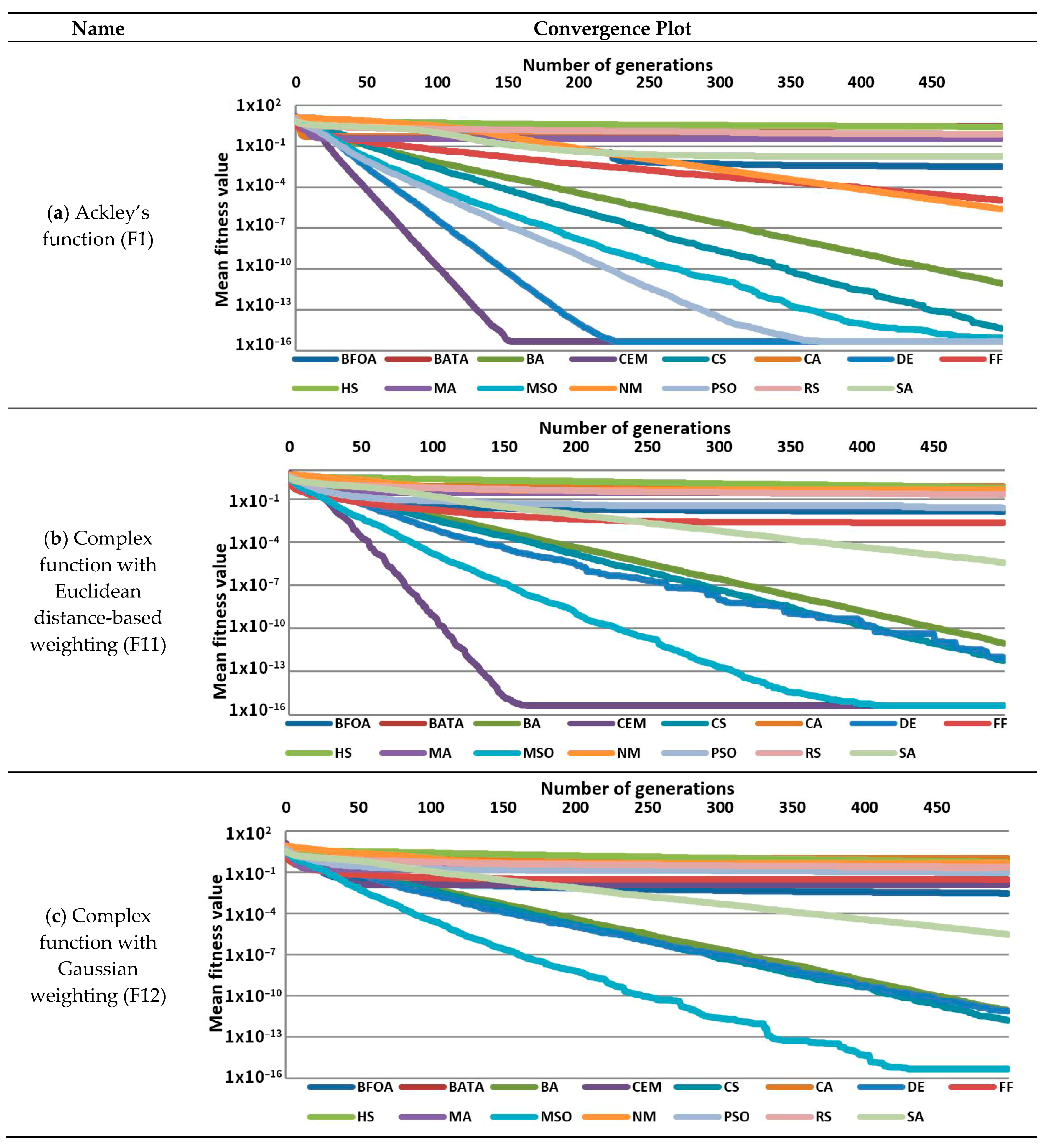
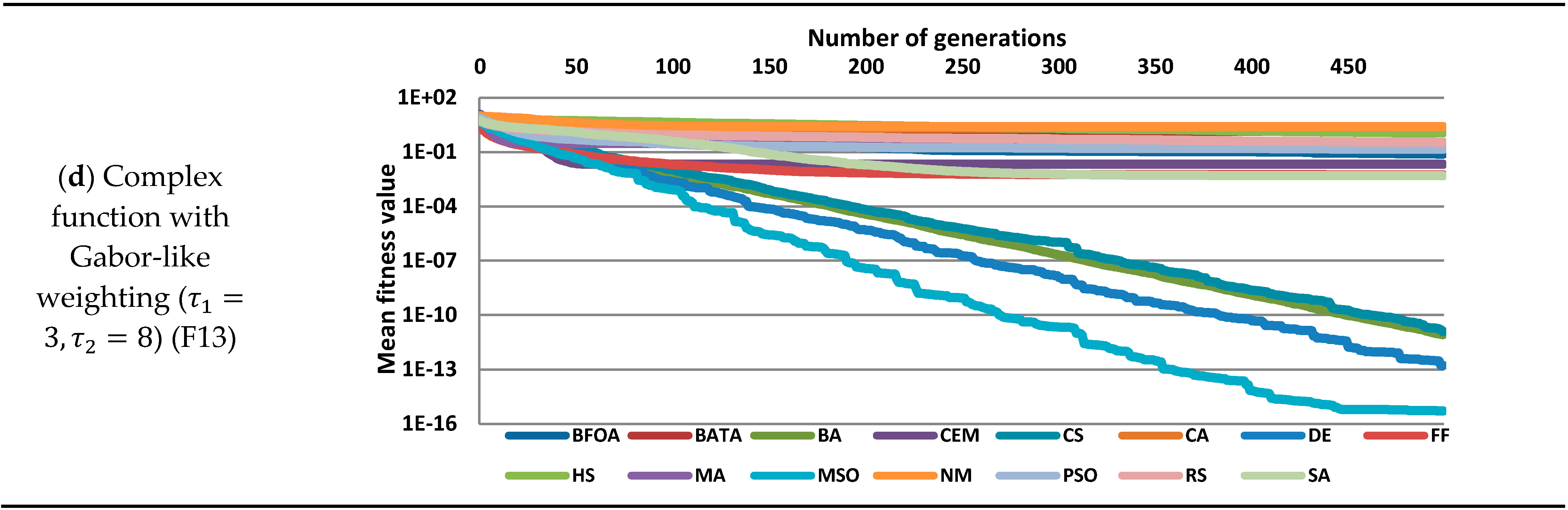
In Figure 2, convergence plots were used to assess the rate of convergence of search algorithms. The responses are normalized from 0 to 100, with 0 representing the best and 100 representing the worst. The convergence rate measures how quickly metaheuristic algorithms can find the best solution. The data points represent the best fit in each iteration as averaged over 100 Monte Carlo simulations. The efficiency of the algorithms is shown in Figure 2. The top five best performance algorithms are listed below (the number denotes the number of solutions found for the 13 test functions):
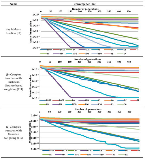
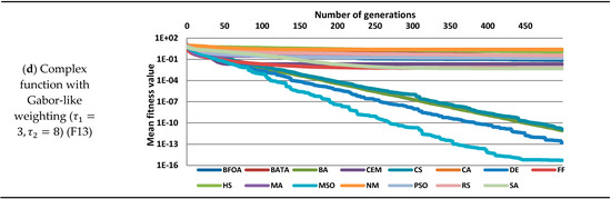
Figure 2.
Convergence plots for Ackley (F1) and Complex (F11. F12. F13) functions. (a) ackley’s function; (b) complex function with Euclidean distance-based weighting; (c) complex function with Gaussian weighting; (d) complex function with Gabor-like weighting (τ1 = 3, τ2 = 8).
Multi-Swarm Optimization (MSO) (13)
Cuckoo Search Algorithm (CS) (12)
Bees Algorithm (BA) (11)
Particle Swarm Optimization (PSO) (9)
Cross-Entropy Method (CEM) (8)
5.2. Assessment of Benchmark Results, Algorithms’ Strengths and Weaknesses
We used fifteen distinct search methods to answer the thirteen benchmark tasks. Unimodal and multimodal issues with varying numbers and distributions of local extremes, as well as unimodal and multimodal problems with varying numbers and distributions of local extremes, were among the aspects of the test functions. Using the software that was built, three challenging benchmark tasks were generated. After analyzing a considerable amount of statistical data, overall performance of the algorithms became apparent. Figure 2 demonstrates the advantages of swarm intelligence techniques. Multi-Swarm Optimization was used to find the global optima in every case (MSO).
On the other hand, even for complicated and noisy functions, Cuckoo Search (CS) and the Bees Algorithm (BA) almost always found the global optima. The Cross-Entropy Method (CEM) and Particle Swarm Optimization (PSO) were less reliable, but they were still highly efficient. In addition, the Cross-Entropy Method and Simulated Annealing (SA) worked excellently; nevertheless, they occasionally remained trapped in local optima. Increasing the number of iterations to enhance the performance of slowly convergent algorithms (HS, SA), convergence charts in Figure 2 show how fast things are coming together. The best algorithms have a rapid convergence rate, which has been shown to be crucial for success.
According to the convergence charts, the weighting functions have a considerable influence on the complexity of complicated functions. According to the mean fitness function values, the complex function with Euclidean distance-based weighting (F11) was more challenging to solve than the simple function (F1). Using the Gaussian weighting function, on the other hand, resulted in smoother edges, reducing the number and distribution of local extremes, making it easier for search engines to identify the global optima. The Complex function with Gabor-like weighting was arguably the most challenging test function since the weighting function produced so much noise.
The best method in this test case was Multi-Swarm Optimization, although its solution was inferior to Euclidean distance-based weighting. Finally, complicated functions with varying weightings have proven to be significant benchmark difficulties.
6. Determining the Optimal Dimensions of the Main Girder of an Overhead Travelling Crane
The overhead crane is one of the most widely used forms of lifting equipment in modern industry. The main purpose of the crane is to handle and transport large loads from one area to another. In addition to lifting large objects, it is capable of short-term horizontal movement, servicing an area of floor space within its travel limitations.
In manufacturing and logistics, where productivity and downtime are important, overhead cranes are widely used. They may transport items between factories, warehouses, and rail and port freight yards. The parallel runways of the crane are usually supported by steel or concrete columns or the reinforced walls of the facility. Moreover, because the bridge construction is elevated above ground level, it only takes up a small quantity of valuable real estate. The distance between the runways is bridged by a moving bridge, which may roll on its powered wheels. With the trolley, the lifting component of the crane, known as the hoist, moves along the bridge rails.
The girder, the principal load-bearing component of the structure, is a critical component of the travelling bridge. In terms of girder count, single and double girder structures are the most prevalent. The girders are usually composed of structural steel. The dimensions of the primary girder must be established during the planning stage of the crane. To keep production and running costs low, the dead weight of the girder must be maintained to a minimum. The bridge crane, on the other hand, must be able to operate consistently throughout its lifetime [40]. Excessive use of safe coefficients can lead to material waste and energy consumption, among other things [41].
This study improved a double-welded box type girder made of a structural steel plate. For an overhead crane, the main girders optimization is a nonlinear, constrained optimization problem. The penalty function approach was used to determine the optimum solution. To solve optimization challenges for robotic arm design, several methods with penalty functions were employed [42].
6.1. The Optimum Design Mathematical Model
A mathematical model of optimization should be supplied to address the mean girder design problem of the overhead crane. All of the choice variables, constraints, and goal functions have been determined.
6.1.1. Decision Variables
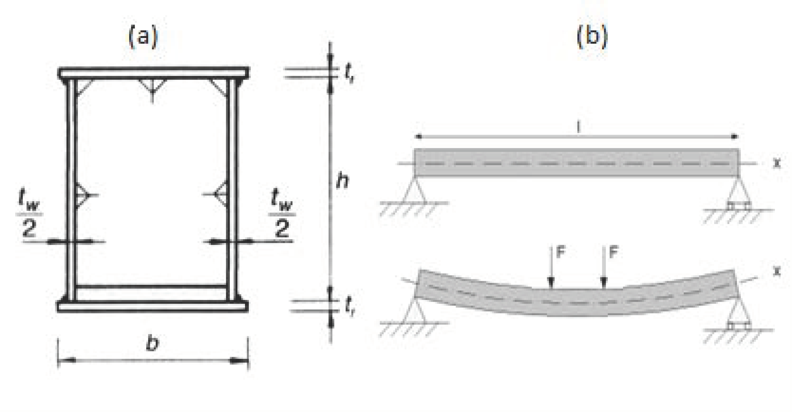
Four variables, [43], can be used to characterize the dimensions of the double-welded box-type girders of the overhead crane. Figure 3 illustrates this.
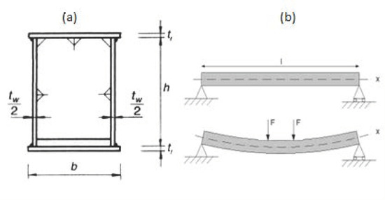
Figure 3.
The decision variables of the design problem. (a) The cross section (b) The whole structure with loadings and deformation.
6.1.2. Constraints
On the four decision variables, min and max limits must be determined (Constraints F1, F2, F3, F4):
The fatigue (Constraint F5) constraint is defined by Eurocode 3 [44]
where is the varying bending moment, is a dynamic factor, is the varying vertical load, is the span length of the main girder. is the length of the trolley, is the elastic section modulus, is the moment of inertia, is the fatigue stress range corresponding to the given cycles of N ( and is a safety factor (according to Eurocode 3 [44], .
The static stress (Constraint F6) is calculated as follows:
where is the static stress, is the yield stress, , are safety factors, is the cross-sectional area (), is the volumetric mass density, is the gravitational acceleration, is the uniform vertical load on the sidewalk, is the uniform vertical load of the rail, and is the weight of the actuating machinery (chassis, drive, engine).
The flange buckling (Constraint F7):
The web buckling (Constraint F8):
The deflection (Constraint F9) is defined by:
where is the elastic modulus of the steel.
6.1.3. Objective Functions
It is a single-objective problem since the optimization aims to find the minimum mass of the main girder m. The cross-sectional area, which is defined by the objective function and design factors, is proportional to the mass [45].
The objective function with penalty is as follows:
where the limit . Where rk is the penalty parameter, are the violated inequality constraints.
6.2. Mathematical Modelling of the Optimum Design Problem
The metaheuristic algorithm collection was used to solve this structural optimization issue using the same input parameters as in Table 2. Metaheuristic methods were used to conduct 100 Monte Carlo searches. For each search, the maximum number of iterations was set at 1000. To avoid the violation of restrictions, a penalty function was created (see Equation (25)).
The following data were given: =2, =240.000 (N), = 20.000 (mm), = 1.900 (mm), . = 69.8 (MPa), . = 1.35, for Fe 360 steel, the yield stress is . = 1.1, . =1.35. = 7.85 ,
= 9.81 (m/, = 1 = 0.2 = 30 kN, = .
Table 6 and Table 7 describe the optimum dimensions of welded box type girders and the accompanying constraint values. The best result is shown in bold letters.
Table 6.
Optimum dimensions of the welded box type main girder.
Table 7.
Corresponding constraint values to optimum dimensions.
Despite the fact that the Firefly Algorithm (FF) provided the optimum solution, the variations in the outcomes were small. The weight difference between the best (Firefly Algorithm, 7524.309 kg) and worst (Memetic Algorithm, 7621.546 kg) solutions was merely 97.237 kg, or less than 2% of the mass of the main girder. The small variance in the results indicates that all of the algorithms were implemented successfully. The values of the constraints in Table 7 further verify the correct operation of the metaheuristic algorithms since the most significant restrictions were fatigue 66.48, static stress 213.64, flange buckling 42, web buckling 124, and deflection 66.67.
The Brute Force method was used to determine the optimal measurements for future evaluation of the main girder of the overhead crane. Brute Force examined all possible options; however, the continuous variables must be discretized in order to obtain the results in an acceptable period of time. Even still, evaluating the 3.237.480.000 possible options took 70 min (4,149,129,594 ms). The best configuration is h = 1240 mm, tw/2 = 20 mm, b = 681 mm, tf = 17 mm, with a main girder weight of 7,528,778 kg. When the findings of the metaheuristic algorithms were compared to the results of Brute Force approach, it was revealed that the metaheuristic algorithms generated superior results.
The Firefly algorithm discovered a better answer in two seconds less time than the Brute Force technique, which took 70 min. The rounding of continuous variables resulted in a discrepancy of 4 kg. If the production of the main beam is planned, the continuous values in the main beam should be discretized using the findings of the Firefly algorithm.
7. Discussion and Future Research
Numerical optimization is a rapidly developing field of research. Several novel evolutionary optimization techniques have recently surfaced. A software solution has been created that allows for the creation of arbitrarily complicated and sophisticated test procedures. In this study, fifteen optimization algorithms with thirteen test functions were benchmarked before being applied to a real-world technical design challenge: finding the optimal dimensions of the main girder of an overhead crane. A comparison with the Brute Force method was carried out. We used fifteen distinct search methods to answer the thirteen benchmark tasks. Unimodal and multimodal issues with varying numbers and distributions of local extremes, as well as unimodal and multimodal problems with varying numbers and distributions of local extremes, were among the aspects of the test functions. Using the software that was built, three challenging benchmark tasks were generated. After analyzing considerable statistical data, the overall performance of the algorithms became apparent. At the test functions, we have elaborated three different weighting functions to introduce noise, making the optimization more difficult. It is critical, however, not to stray from the original optimal settings to be comparable. According to the convergence charts, the weighting functions significantly influence the complexity of complicated functions. The complex function with Euclidean distance-based weighting (F11) was more challenging to solve than the simple function, according to the mean fitness function values (F1). The Gaussian weighting function, on the other hand, produced smoother edges by reducing the number and distribution of local extremes, making it easier for search engines to identify the global optima. Because the weighting function produced so much noise, the Complex function with Gabor-like weighting was arguably the most challenging test function.
The test functions, as well as the crane girder design, show that evolutionary optimization techniques are powerful design tools. Based on these 13 test examples, Multi-Swarm Optimization (MSO), the Cuckoo Search method (CS), the Bees Algorithm (BA), and Particle Swarm Optimization (PSO) are the most efficient optimization algorithms. For crane girder optimization, the Firefly algorithm (FF) performed best. So we cannot declare that in all cases there is one algorithm which is the most efficient.
We intend to develop more difficult, self-made test issues in the future, as well as compare and contrast alternative metaheuristic techniques as were shown in [37,38,39]. Based on the benchmark findings, novel, more efficient hybrid metaheuristic algorithms have been created, which might be applied in real-world structural and system optimization issues, as in recent publications [46,47,48]. Naturally, the development of the optimization techniques never stops; existing techniques are modified to be more efficient, as recently in [49].
8. Conclusions
Those who are making structural optimization consistently seek reliable and quick algorithms to elaborate optimization. There are a significant number of techniques available. All authors declare that his/her algorithm is better than the others. The different test functions were to evaluate the performance of these algorithms. We have introduced Euclidean distance-based weighting, Gaussian weighting, and Gabor-like weighting to render the test more challenging. These noisy test functions selected the optimization techniques better than the simple test functions. On the other hand, it is clear that no optimizer exists which has the best performance in all cases and at all types of problem-solving. In any case, we have demonstrated which are the most efficient optimizers at our test function range. This can help users to choose their own method. Finally a real-world problem, the crane girder design, shows the applicability of these techniques.
Author Contributions
Conceptualization, K.J., C.B. and G.Z.M.; methodology, K.J., C.B.; software, G.Z.M. and C.B.; formal analysis, K.J. and C.B.; writing—review and editing, K.J., C.B. and G.Z.M.; supervision, K.J.; project administration, K.J. All authors have read and agreed to the published version of the manuscript.
Funding
The research was supported by the Hungarian National Research, Development and Innovation Office under the project number K 134358.
Institutional Review Board Statement
Not applicable.
Informed Consent Statement
Not applicable.
Data Availability Statement
The data presented in this study are available on request from the corresponding author.
Acknowledgments
We would like to express gratitude for the help and advice of László Kota in the optimization.
Conflicts of Interest
The authors declare no conflict of interest.
References
- Liang, Y.-C.; Juarez, J.R.C. A novel metaheuristic for continuous optimization problems: Virus optimization algorithm. Eng. Optim. 2015, 48, 1–21. [Google Scholar] [CrossRef]
- Mologa, M.; Smutnicki, C. Test Functions for Optimization Needs. 2014, pp. 1–10. Available online: http://www.robertmarks.org/Classes/ENGR5358/Papers/functions.pdf (accessed on 24 May 2020).
- Liang, J.; Suganthan, P.; Deb, K. Novel composition test functions for numerical global optimization. In Proceedings of the Proceedings 2005 IEEE Swarm Intelligence Symposium, Pasadena, CA, USA, 8–10 June 2005; IEEE: Piscataway, NJ, USA, 2005; pp. 68–75. [Google Scholar]
- Barcsák, C.; Jármai, K. Benchmark for testing evolutionary algorithms. In Proceedings of the 10th World Congress on Structural and Multidisciplinary Optimization WCSMO10, Orlando, FL, USA, 19–24 May 2013. [Google Scholar]
- Ghafil, H.N.; Jármai, K. Dynamic differential annealed optimization: New metaheuristic optimization algorithm for engineering applications. Appl. Soft Comput. 2020, 93, 106392. [Google Scholar] [CrossRef]
- Smairi, N.; Siarry, P.; Ghédira, K. A hybrid particle swarm approach based on Tribes and tabu search for multi-objective optimization. Optim. Methods Softw. 2015, 31, 204–231. [Google Scholar] [CrossRef]
- Hasançebi, O.; Kazemzadeh Azad, S. Discrete size optimization of steel trusses using a refined big bang–big crunch algorithm. Eng. Optim. 2014, 46, 61–83. [Google Scholar] [CrossRef]
- Kaveh, A.; Bakhshpoori, T. A new metaheuristic for continuous structural optimization: Water evaporation optimization. Struct. Multidiscip. Optim. 2016, 54, 23–43. [Google Scholar] [CrossRef]
- Yousefikhoshbakht, M.; Didehvar, F.; Rahmati, F. Solving the heterogeneous fixed fleet open vehicle routing problem by a combined metaheuristic algorithm. Int. J. Prod. Res. 2014, 52, 2565–2575. [Google Scholar] [CrossRef]
- Zavala, G.R.; Nebro, A.J.; Luna, F.; Coello, C.A.C. A survey of multi-objective metaheuristics applied to structural optimization. Struct. Multidiscip. Optim. 2014, 49, 537–558. [Google Scholar] [CrossRef]
- Zavala, G.; Nebro, A.J.; Luna, F.; Coello, C.A.C. Structural design using multi-objective metaheuristics. Comparative study and application to a real-world problem. Struct. Multidiscip. Optim. 2016, 53, 545–566. [Google Scholar] [CrossRef]
- Karakostas, S. Multi-objective optimization in spatial planning: Improving the effectiveness of multi-objective evolutionary algorithms (non-dominated sorting genetic algorithm II). Eng. Optim. 2015, 47, 601–621. [Google Scholar] [CrossRef]
- Brownlee, J. Clever Algorithms: Nature-Inspired Programming Recipes; Lulu: Morrisville, NC, USA, 2011; pp. 27–336. [Google Scholar]
- Liu, Y.; Passino, K. Biomimicry of Social Foraging Bacteria for Distributed Optimization: Models, Principles, and Emergent Behaviors. J. Optim. Theory Appl. 2002, 115, 603–628. [Google Scholar] [CrossRef]
- Yang, X.S. A New Metaheuristic Bat-Inspired Algorithm. In Nature Inspired Cooperative Strategies for Optimization (NISCO 2010); González, J.R., Pelta, D.A., Cruz, C., Terrazas, G., Krasnogor, N., Eds.; Studies in Computational Intelligence; Springer: Berlin, Germany, 2010; pp. 65–74. [Google Scholar]
- Pham, D.T.; Ghanbarzadeh, A.; Koc, E.; Otri, S.; Rahim, S.; Zaidi, M. The Bees Algorithm; Technical report; Manufacturing Engineering Centre, Cardiff University: Cardiff, Wales, 2005. [Google Scholar]
- Rubinstein, R.Y. Optimization of computer simulation models with rare events. Eur. J. Oper. Res. 1997, 99, 89–112. [Google Scholar] [CrossRef]
- Yang, X.S.; Deb, S. Cuckoo search via Lévy flights. In Proceedings of the World Congress on Nature & Biologically Inspired Computing (NaBIC 2009), Coimbatore, India, 9–11 December 2009; IEEE Publications: Piscataway, NJ, USA, 2009; pp. 210–214. [Google Scholar]
- Reynolds, R.G. An introduction to cultural algorithms. In Proceedings of the 3rd Annual Conference on Evolutionary Programming, San Diego, CA, USA, 24–26 February 1994; World Scientific Publishing: Singapore, 1994; pp. 131–139. [Google Scholar]
- Storn, R.; Price, K. Differential Evolution: A Simple and Efficient Adaptive Scheme for Global Optimization over Continuous Spaces; Technical Report TR-95-012; International Computer Science Institute: Berkeley, CA, USA, 1995. [Google Scholar]
- Yang, X.S. Firefly algorithms for multimodal optimization. In Stochastic Algorithms: Foundations and Applications, SAGA 2009, Lecture Notes in Computer Sciences 5792; Springer: Berlin, Germany, 2009; pp. 169–178. [Google Scholar]
- Carbas, S. Design optimization of steel frames using an enhanced firefly algorithm. Eng. Optim. 2016, 48, 2007–2025. [Google Scholar] [CrossRef]
- Geem, Z.W.; Kim, J.H.; Loganathan, G.V. A new metaheuristic optimization algorithm: Harmony search. Simulation 2001, 76, 60–68. [Google Scholar] [CrossRef]
- Moscato, P. On evolution, Search, Optimization, Genetic Algorithms and Martial Arts: Towards Memetic Algorithms; Technical Report; California Institute of Technology: Pasadena, CA, USA, 1989. [Google Scholar]
- Nelder, J.A.; Mead, R. A Simplex Method for Function Minimization. Comput. J. 1965, 7, 308–313. [Google Scholar] [CrossRef]
- McCaffrey, J. Amoeba Method Optimization using C#. MSDN Magazine, June 2013. Available online: https://docs.microsoft.com/en-us/archive/msdn-magazine/2013/june/test-run-amoeba-method-optimization-using-csharp (accessed on 24 May 2020).
- Kennedy, J.; Eberhart, R.C. Particle swarm optimization. In Proceedings of the ICNN’95—International Conference on Neural Networks, Perth, WA, Australia, 27 November–1 December 1995; pp. 1942–1948. [Google Scholar]
- Kennedy, J. Particle swarm optimization. In Encyclopedia of Machine Learning; Springer: New York, NY, USA, 2010; pp. 760–766. [Google Scholar]
- Clerc, M. Particle Swarm Optimization; John Wiley & Sons: Hoboken, NJ, USA, 2010; Volume 93. [Google Scholar]
- Mortazavi, A.; Toğan, V. Simultaneous size, shape, and topology optimization of truss structures using integrated particle swarm optimizer. Struct. Multidiscip. Optim. 2016, 54, 715–736. [Google Scholar] [CrossRef]
- Zhao, S.Z.; Liang, J.J.; Suganthan, P.N.; Tasgetiren, M.F. Dynamic multi-swarm particle swarm optimizer with local search for Large Scale Global Optimization. In Proceedings of the 2008 IEEE Congress on Evolutionary Computation (IEEE World Congress on Computational Intelligence), Hong Kong, China, 1–6 June 2008; Institute of Electrical and Electronics Engineers (IEEE): Piscataway, NJ, USA, 2008; pp. 3845–3852. [Google Scholar]
- McCaffrey, J. Multi-Swarm Optimization. MSDN Magazine, Vol. 28, No. 9. September 2013. Available online: https://docs.microsoft.com/en-us/archive/msdn-magazine/2013/september/test-run-multi-swarm-optimization (accessed on 19 October 2021).
- Brooks, S.H. A Discussion of Random Methods for Seeking Maxima. Oper. Res. 1958, 6, 244–251. [Google Scholar] [CrossRef]
- Kirkpatrick, S. Optimization by simulated annealing: Quantitative studies. J. Stat. Phys. 1984, 34, 975–986. [Google Scholar] [CrossRef]
- Corana, A.; Marchesi, M.; Martini, C.; Ridella, S. Minimizing multimodal functions of continuous variables with the “simulated annealing” algorithm. ACM Trans. Math. Softw. 1987, 13, 262–280. [Google Scholar] [CrossRef]
- Hasançebi, O.; Çarbaş, S.; Saka, M.P. Improving the performance of simulated annealing in structural optimization. Struct. Multidiscip. Optim. 2010, 41, 189–203. [Google Scholar] [CrossRef]
- Abualigah, L.; Diabat, A.; Mirjalili, S.; Elaziz, M.A.; Gandomi, A.H. The Arithmetic Optimization Algorithm. Comput. Methods Appl. Mech. Eng. 2021, 376, 113609. [Google Scholar] [CrossRef]
- Abualigah, L.; Yousri, D.; Elaziz, M.A.; Ewees, A.A.; Al-Qaness, M.A.; Gandomi, A.H. Aquila Optimizer: A novel meta-heuristic optimization algorithm. Comput. Ind. Eng. 2021, 157, 107250. [Google Scholar] [CrossRef]
- Liang, J.J.; Qu, B.Y.; Suganthan, P.N.; Hernández-Díaz, A.G. Problem Definitions and Evaluation Criteria for the CEC 2013 Special Session on Real-Parameter Optimization; Technical Report 201212; Computational Intelligence Laboratory, Zhengzhou University: Zhengzhou, China, 2013. [Google Scholar]
- Sun, C.; Tan, Y.; Zeng, J.; Pan, J.; Tao, Y. The Structure Optimization of Main Beam for Bridge Crane Based on An Improved PSO. J. Comput. 2011, 6, 1585–1590. [Google Scholar] [CrossRef]
- Zuberi, R.H.; Kai, L.; Zhengxing, Z. Design optimization of EOT crane bridge. In Proceedings of the International Conference on Engineering Optimization, Rio de Janeiro, Brazil, 1–5 June 2008; pp. 192–201. [Google Scholar]
- Ghafil, H.N.; Jármai, K. Optimization for Robot Modelling with MATLAB; Springer Nature: Cham, Switzerland, 2020; 220p. [Google Scholar] [CrossRef]
- Farkas, J.; Jármai, K. Analysis and Optimum Design of Metal Structures; Taylor & Francis: Boca Raton, FL, USA, 2020; pp. 236–239. [Google Scholar]
- Eurocode 3, Design of Steel Structures, Part 1-1: General Structural Rules; CEN: Brussels, Belgium, 2009.
- Farkas, J.; Jármai, K. Optimum Design of Steel Structures; Springer: Heidelberg, Germany, 2013; 288p. [Google Scholar] [CrossRef]
- Ziane, K.; Ilinca, A.; Karganroudi, S.; Dimitrova, M. Neural Network Optimization Algorithms to Predict Wind Turbine Blade Fatigue Life under Variable Hygrothermal Conditions. Eng 2021, 2, 278–295. [Google Scholar] [CrossRef]
- Paggi, M. An Analysis of the Italian Lockdown in Retrospective Using Particle Swarm Optimization Applied to an Epidemiological Model. Physics 2020, 2, 368–382. [Google Scholar] [CrossRef]
- Seyedi, M.R.; Khalkhali, A. A Study of Multi-Objective Crashworthiness Optimization of the Thin-Walled Composite Tube Under Axial Load. Vehicles 2020, 2, 438–452. [Google Scholar] [CrossRef]
- Abbaszadeh Shahri, A.; Khorsand Zak, M.; Abbaszadeh Shahri, H. A modified firefly algorithm applying on multi-objective radial-based function for blasting. Neural Comput. Appl. 2021, 1–17. [Google Scholar] [CrossRef]
Publisher’s Note: MDPI stays neutral with regard to jurisdictional claims in published maps and institutional affiliations. |
© 2021 by the authors. Licensee MDPI, Basel, Switzerland. This article is an open access article distributed under the terms and conditions of the Creative Commons Attribution (CC BY) license (https://creativecommons.org/licenses/by/4.0/).