Article

Existence of Incompressible Vortex-Class Phenomena and Variational Formulation of Raleigh–Plesset Cavitation Dynamics

by
Terry Eleftherios Moschandreou
1,* and
Keith Christian Afas
2
1
Department of Mathematics, University of Western Ontario, London, ON N6A 5C1, Canada
2
School of Biomedical Engineering, University of Western Ontario, London, ON N6A 5C1, Canada
*
Author to whom correspondence should be addressed.
Appl. Mech. 2021, 2(3), 613-629; https://doi.org/10.3390/applmech2030035
Submission received: 11 July 2021 / Revised: 11 August 2021 / Accepted: 25 August 2021 / Published: 29 August 2021
(This article belongs to the Special Issue Mechanics and Control using Fractional Calculus)

Abstract

:
The following article extends a decomposition to the Navier–Stokes Equations (NSEs) demonstrated in earlier studies by corresponding author, in order to now demonstrate the existence of a vortex elliptical set inherent to the NSEs. These vortice elliptical sets are used to comment on the existence of solutions relative to the NSEs and to identify a potential manner of investigation into the classical Millennial Problem encompassed in Fefferman’s presentation. The article also presents the utilization of a recently developed versatile variational framework by both authors in order to study a related fluid-mechanics phenomena, namely the Raleigh–Plesset equations, which are ultimately obtained from the NSEs. The article develops, for the first time, a Lagrangian density functional for a closed surface which when minimized produced the Raleigh–Plesset equations. The article then proceeds with the demonstration that the Raleigh–Plesset equations may be obtained from this energy functional and identifies the energy dissipation predicted by the proposed Lagrangian density. The importance of the novel Raleigh–Plesset functional in the greater scheme of fluid mechanics is commented upon.

1. Introduction

Fluid Mechanics is a field that posesses diversity in approaches, solutions, and versatility. The crown jewels of the field of fluid mechanics—the Navier–Stokes equations (NSEs)—are among some of the most impactful mathematical equations. In addition, while the principles forming the NSEs rely on intuitive conservation principles from continuum mechanics, such as the conservation of mass and momentum, the resultant NSEs describing the general motion of fluids is immensely complex. NSEs often do not admit analytic solutions without perturbation analysis or asymptotic approximations. As such, their existence and uniqueness remain elusive as the motivation of the famed Millennium Problem, proposed by Fefferman in 2008 [1]. One phenomenon that arises from the NSEs, vortex or pattern formation, is caused by non-linear interactions in complex fluid systems. It has been observed that by prescribing initial conditions in terms of a Fourier series, it is possible to trigger instabilities from a primary static pattern determined by particular initial conditions. This is amenable to treatment on a 3D torus or lattice of periodic cells [2], (see [3] for Geometric Algebra technique also used in cylindrical co-ordinates); these instabilities can be analyzed as strong indicators of a possible transition to disorder [4].
In general, instabilities can be represented by saddle points of the associated system, and the same may be extended to the Navier–Stokes system. For example, networks of webs of saddle points have been shown to exist for the Kuramoto–Sivashinsky equation [5,6] with similar possibilities for the Navier–Stokes equations; saddle points in general are associated with unstable solutions of PDE systems, which are the prototypical example of local instability analysis given in earlier computational studies [7]. Various instabilities may occur that eventually develop into turbulence with vortices and eddies and in some cases result in spatio-temporal chaos (STC) [8]. Moving saddle points play an important role in turbulent dynamics, and strong turbulent motion is connected and related to saddle point analysis. Recent work on incompressible flows, velocity-pressure correlation, and global regularity can be observed in earlier studies [9], as well as time dependent flows of the two dimensional NSEs on a Torus [10]. While the NSEs are generally accepted as the prime governing equations in fluid analysis, there has been a push throughout centuries to propose alternative models that address specific fluid processes in a manner where they consistently admit analytic results. These alternative models may be shown to either draw from the NSEs or be phenomenologically derived; in the latter case, phenomenological models may be validated to mimic numerical predictions from the NSEs with small deviations, although not being obtained from the NSEs. Consequentially, it is difficult to determine if phenomenological models encompass conservation principles implicitly.
One field of research that enjoys such alternative models is the field governing matter transitions, such as those that study the dynamics of fluid inclusions, informally referred to as “bubbles” [11]. Bubbles have a rich history in fluid mechanics and soft condensed matter physics, as well in fields of mathematics such as differential geometry. Their attention from several fields of research originates due to the versatility of their geometries and the simplicity of their physics principles. One of the earliest studies on bubbles was performed in the early 19th century and culminated in the Young–Laplace Equation [12].
R = 2 γ Δ P
The equation, relating the steady-state radius R of a homogeneous spherical bubble to its surface tension γ and pressure differential with its exterior Δ P , was well formulated by Thomas Young and Pierre Simon de Laplace. In 1830, the connection to differential geometry was made by Carl Friedrich Gauss by realizing the spherical radius as the membrane’s curvature, establishing the equation in its celebrated form today. The Young–Laplace–Gauss equation culminated in the realization that bubbles were affected by surface tension and pressure, which locally affected its curvature. This connection to differential geometry emphasized that bubbles are, in themselves, not only phenomenon relating to the NSEs but also distinct geometrical entities simultaneously. The realization of the relation between the Young–Laplace-Gauss equation to the NSEs occurred through the work of Lord Raleigh and Milton Plesset in the 20th century, culminating in the Raleigh–Plesset equation. This equation extends the Young–Laplace–Gauss equation from being able to predict steady-state radius, to being able to predict a time-varying bubble radius; therefore, the non-linear Raleigh–Plesset equation is most often used for cavitation dynamics. The equation was obtained in the 20th century by a thorough application of the NSEs, assuming a cavity with a pressure difference, an external liquid with a pre-specified density and viscosity, and incorporating boundary conditions [13]. Using these observations, an approximation to the NSEs resulted in the following non-linear ODE for the spherical radius R ( t ) of a cavitation bubble.
ρ L R t 2 R + 3 2 t R 2 Momentum Term + 4 ν L ρ L R t R Viscosity Term + 2 γ R + Δ P Young - Laplace = 0
In the steady-state case where t = 0 , the Young–Laplace equation emerges. While the Raleigh–Plesset equation accomplishes much in understanding cavitation dynamics, one of the critical consequences is that the relation to differential geometry is lost since the equation is derived from the NSEs. What is lost is the application to non-spherical surfaces or even non-closed geometries; this is because the dynamics of such surfaces are matters pertaining to differential geometry and not exclusively to the NSEs. In addition, it is difficult to observe how the equation might be generalized further to more complex fluid mechanics matters; an example is the spontaneous emergence of eddies and vortices present in 2D incompressible fluids. This has been commented on in earlier studies [14], however, the additional presence of cavitation dynamics is difficult to relate to the field of vortex dynamics, which itself is a phenomenological sub-branch of fluid mechanics.
One possible solution is to provide an alternative derivation of the Raleigh–Plesset equation from a starting point other than the NSEs. Such a derivation would simply require a framework that is geometrical in nature, accommodates for kinetic processes, and has physical conservation principles embedded in its framework or, at the very least, implementable as constraints. Such framework, developed in 2019, has the potential to predict the evolution of surfaces, subject to an energy functional, and also permits the implementation of constraints requiring a conservation of surface area and/or volume [3]. This framework was formulated under the assumption of invariance under the calculus of moving surfaces (CMS) and, as such, is especially well suited for considering the time-evolution of irregular geometries, which may be intractable by modern physics. Not only would a derivation of the Raleigh–Plesset Equation using this CMS variational framework open up the possibility of a method to treat fluids outside of the NSEs, but it would also allow for the analysis of cavitation and other processes within incompressible eddies and vortices.

2. Onset of Turbulence: Eddies and Vortices in Incompressible Fluids

In this section, a general presentation of a solution of the incompressible NSEs is given, and the existence of instabilities resulting in the formation of eddies and vortices in incompressible fluids is demonstrated by showing that there exists saddle points and possibly limit cycles (attractors that are closed orbits). The analytical solution of the NSE’s presented in this paper is expressed as an asymptotic series in terms of its asymptotic variable, which can be integrated a second time, term by term with respect to the time to obtain time varying spatial variables in the phase portraits examined. Considering a cubical lattice, the presence of singularities is also addressed by using the concept of rotund surfaces.

2.1. Three-Dimensional Incompressible Navier–Stokes Equations

The 3D incompressible unsteady Navier–Stokes Equations (NSEs) in Cartesian coordinates may be written in the form for the velocity field u * = u * i e i . , . u * i = { u x * , u y * , u z * } :
ρ t * + u * j * j u i * μ * 2 u i * + * i P * = ρ F i *
where ρ is constant density, μ is dynamic viscosity, and F * = F * i e i are the body forces on the fluid. The components of the velocity vector and pressure in u = ( u ) i e i , P = ( P ) i e i , coordinates x i , and time t are reparametrized according to the following form utilizing the non-dimensional quantity δ (assumed negative and such that | δ | is arbitrarily small).
u i * = 1 δ u i . , . P i * = 1 δ 2 P i . , . x i * = δ x i . , . t * = δ 2 t
Along with Equation (3), the continuity equation in Cartesian coordinates is given in tensor index notation by the following.
i u i = 0

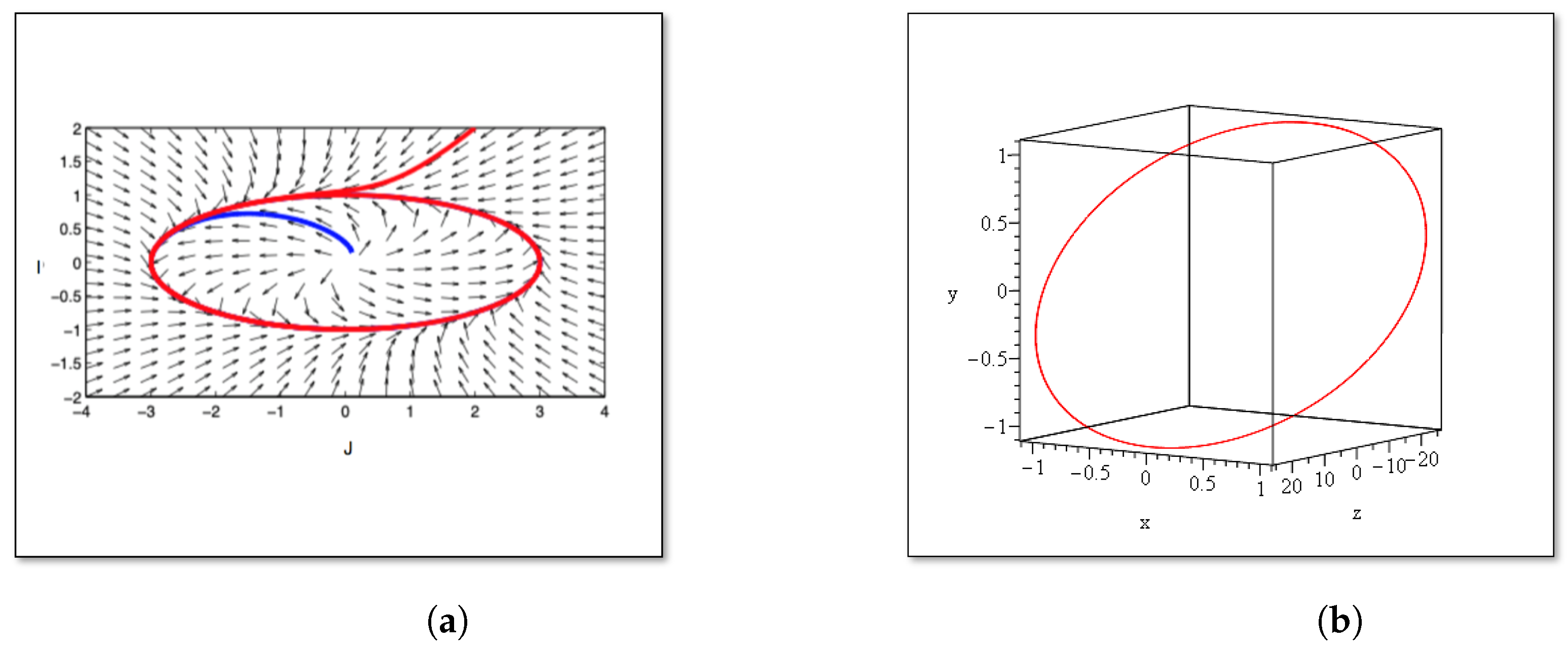
2.2. Decomposition of NSEs, Limit Cycles, and Vortices

Equation (3) together with Equation (5) and using the initial condition of u * ( x * , 0 ) = ξ ( x * ) such that · ξ = 0 encompass the NSEs along with an incompressible initial condition. Ensuring periodic boundary conditions specified in [1] defined on a cube domain Ω with the associated lattice in R 3 is referred to as the periodic BVP for the NSEs in R 3 . It has been shown in earlier NSE work [2] that a solution for Equation (3) with transformation given by Equation (4) exists in the following form:
u = ( u x , u y , u z ) : R 3 R 3
where u z in Equation (6) satisfies the following integral equation.
t u z z + 1 u z 2 u z 2 · b t + ( 1 δ 1 ) 1 u z 2 u z t 2 + 1 u z 2 u z u z z u z t + μ ρ 1 u z 2 ( 1 1 δ ) u z t 2 u z + ( 1 δ 1 ) 1 ρ 1 u z 2 u z t P z + 1 u z 2 S 1 δ ρ u z 2 x y P + b 1 ρ u z P z · n d S + δ 2 1 u z 2 F T · u z 2 1 u z 2 δ 3 u z u z t u z z F z + δ 3 b · ( u z F z ) = 1 b u z 2 U u z t b · b u z d V
Here, it is assumed that b from Equation (7) is given by the following:
b = 1 δ u x i + 1 δ u y j
and δ is arbitrarily small. The x , y force is F T = ( F T 1 , F T 2 ) and the z force is F z . It is worth noting that Poisson’s Equation can be written as in [2].
1 ρ P z z = ( 1 2 u z 2 ) + u z x 2 + u z y 2 u z x y 2 u z 2 z t uz + 3 z 3 uz
It was shown in [2] that since the following is the case:
P x x + P y y = 2 z t uz x , y , z , t + 3 z 3 uz x , y , z , t ,
then the following results.
1 ρ P = ( 1 2 u z 2 ) + u z x 2 + u z y 2 u z x y 2 u z
By solving for P z in Equation (7) and differentiating with respect to z, we obtain P z z which gives a PDE in terms of u z and b alone. Multiplying Equation (7) by δ and letting u z = u z * δ . It follows that δ 2 and higher order terms are set to zero for small δ . The solution obtained (in terms of z, that is H ( z ) further below) can be returned to u z at the end since there are constants for the solution obtained, that is C 1 , C 2 C 3 for H and lifting constant F 0 (see Equation (13) below) which can be rescaled as C i = C ˜ i / δ and F 0 = F ˜ / δ . So small negative delta works as well as large delta and the system is completely ordered. The following can be determined,
u x = C * sin 4 t * x δ 2 + cos 4 t * + 2 y δ 2 . u y = C * cos 4 t * 2 x δ 2 sin 4 t * y δ 2
where C * = 1 δ 2 is a real valued scaling constant. Here, the velocity b is a kinematic benchmark example for testing the vortex criteria [14]. Moreover, u z z = · b 0 . It is an indeterminate form 0 / 0 at δ = 0 . Solving for u z in Equation (7) produces a class of solutions G i . Here, the defining equations are in terms of the vorticity components in 3D. Since u x and u y are z-independent, the vorticity component equations for a constant vorticity are u z x = C , u z y = C and u y x u x y = C . It has been shown in [2] and detailed in the Appendix A that u z may be given by the following:
u z = F 0 + F ( x , y ) H ( z ) × G ( y , 8 c 3 y ( sin ( 4 t ) cos ( 4 t ) ) e 2 c 3 ( sin ( 4 t ) cos ( 4 t ) ) d t + x e 2 c 3 ( cos ( 4 t ) sin ( 4 t ) ) )
where F 0 R + is a lifting constant, and the following is the case.
H = C 1 + C 2 e z c 3 + C 3 e z c 3
In addition it should be noted that F ( x , y ) is a general function to be determined, C 1 , C 2 , C 3 and c 3 are arbitrary constants, and G belongs to a general family of functions. The elements of the family of solutions G have a second partial derivative with respect to t equal to zero since, by a dimensional argument, the jerk vector is zero for arbitrarily small δ . The full expression for G is shown here to be exactly in the following form:
G = exp 1 8 i 8 e 4 it 2 c 3 cos 4 t + 2 c 3 sin 4 t c 3 iy e 8 it + ix + e 8 it x + y dt
where i = 1 . In the first part of this paper, the long-run behaviour of the trajectories of the associated dynamical system of the equivalent form for the 3D Navier–Stokes Equations (found in Equations (3) and (4)) — that is, Equation (7)— is proven to exist, and it is shown that the trajectories for n = 3 converge in time to a closed orbit of period T in each cell of the lattice. The system is also shown to have saddle points and orbits for which its interiors are saddle surfaces. Before the proof of the main result, some preliminary definitions and notations are introduced.
Solutions are obtained in nonstarred variables first, and then the results are shown in Figure 1 for starred variables.
An upper bound for the integral can be expressed as follows. The arithmetic mean-geometric mean inequality for complex numbers is used here [15]. Let ϕ ( 0 , π / 2 ) and W ϕ = { z C : | arg z | ϕ } . Then, for all z 1 ,…, z n W ϕ , we have the following:
k = 1 n | z k | 1 n σ ( 1 n [ n 2 ] , cos ( 2 ϕ ) ) 1 n k = 1 n z k
where the following results.
σ ( μ , a ) = 2 ( 2 μ ) μ a ( 2 μ 1 ) + 4 μ ( 1 μ ) + a 2 ( 1 2 μ ) 2 μ 2 ( 1 μ ) + a 2 ( 2 μ 1 ) + a 4 μ ( 1 μ ) + a 2 ( 1 2 μ ) 2 1 / 2
For n = 2 , there is a summative bound on the product of the two complex functions z 1 and z 2 in Equation (16).
z 1 = 1 8 i 8 e 4 i t 2 c 3 cos 4 t + 2 c 3 sin 4 t z 2 = c 3 i y e 8 i t + i x + e 8 i t x + y 1
Here, the terms in Equation (18) appear in Equation (15). The following chain of inequalities results for the modulus of the complex function a t exp w ( s ) d s in which w = z 1 z 2 :
a t e w ( s ) d s a t e w ( s ) d s a t e w ( s ) d s
a t e w ( s ) d s = a t e z 1 z 2 d s a t e ζ z 2 d s
where ζ = sup K z 1 and K = s R | a s t ] . The upper bound at the end of the chain in Equation (19) has a closed form antiderivative. It is shown in this paper that there potentially exists a limit cycle that converges to an orbit associated with a saddle surface. It has been verified that a t e ζ z 2 d s has existing saddle points that are secondary instabilities emerging from a stationary periodic structure. Integral evaluation is immediate in terms of exponential integral function. Furthermore, this solution can be integrated to obtain e ζ z 2 d t d t . This may be obtained by using an asymptotic series expansion for large parameter c 3 found in most symbolic and numerical libraries (i.e., Maple 2021’s asympt command).
In the result of Figure 1c,d, c 3 δ 1 due to symmetry of H ( z * ) in Equation (14). Here, in the limit it is δ 0 , c 3 . Finally, since an upper bound is established which are the closed orbits, it can only be concluded that the field lines are attracted to the closed orbit from within it, starting at the zero vector in R 3 toward a maximum or on the other side towards a minimum. An example of a limit cycle is shown in Figure 2.
In Figure 2b, a slanted elliptical limit cycle can be observed to be plotted along coordinates I and J, which are oblique coordinates. The embedding of this elliptical limit set in R 3 can be observed in Figure 2b.

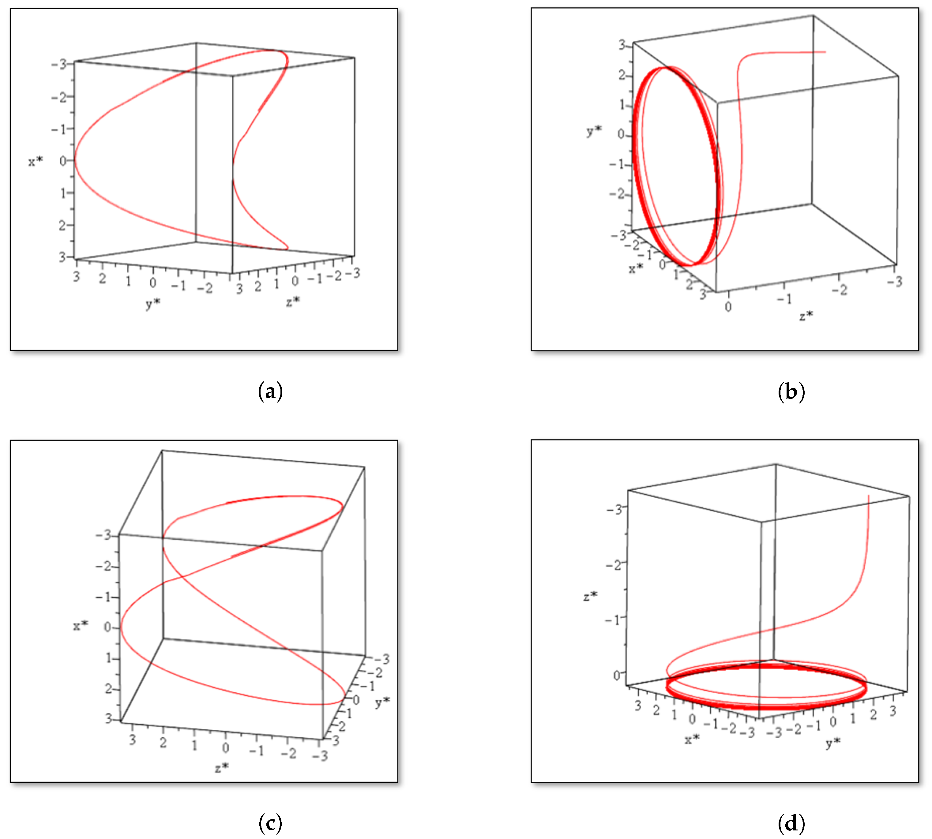
2.3. Convergence and Singularities of Incompressible Eddies and Vortices Along Edge of Cube Lattice

An important criterion for proving that a sequence of real numbers converges without knowing its limit is named the Cauchy criterion.
Definition 1.
Suppose { S n } n = 1 is a sequence of real numbers. Then { S n } n = 1 is called a Cauchy sequence if for any ϵ > 0 there exists an N I such that the following is the case,
| S m S n | < ϵ ( m , n N ) .
The Cauchy criterion is used to show that spacecurves ( x * ( t ) , y * ( t ) , z * ( t ) ) parametrized in t(time) converging to the orbit in Figure 1 is a closed periodic orbit. In Maple 2021, this was shown by keeping a length of interval fixed at say two units in t and shifting the interval towards very large values. The measure of the interval stays the same but the orbit generated converges (to Figure 1a,c). In Figure 1b,d, the limit of the integral of solution as c 3 approaches infinity was obtained explicitly to achieve the portrait in order to show that the attracting set is a two dimensional set and to show that an arbitrarily small c 3 , which is an amplitude that becomes arbitrarily large, gave way to a swirling orbit towards minus infinity for z * (Figure not shown). There is the question of singularities occurring along the edges and at corners of a cube lattice. A cube in the lattice can be transformed into a slight rotund ball by slightly rounding its vertices and edges and puffing out its facets. Then, the supporting lines and planes of Ω can be regarded as tangents, each one touching the surface of Ω at one and only one point [16]. A continuous one-to-one relationship exists between tangents relative to the rotund boundaries of Ω and the points of tangency [16]. If Y T is a tangent unit functional on Ω ( Y is a vector), and x is a unit vector that is a point of tangency on the surface of Ω , then the following differentiation of the norm of x holds.
d x = Y T d x / x
Equivalently, one finds differentiation with respect to t:
d x d t = Y T d x d t / x
where T is the transpose of the vector Y . Recalling G in Equation (15) and the ensuing velocity function u z , it is clear that the following is the case:
x 3 = u z d t
where x 3 is the z-component of x . Substituting for Y 3 = u z and x 3 in Equation (24) into Equation (23), the following is the case.
u z 2 = 1 2 d x 2 d t
Let N = x 2 . The energy equality for incompressible NSE’s as used in [2,17] is the following:
d u 2 d t = 2 ν u 2
where ν is the viscosity of the fluid. Substituting u x , u y , and u z into Equation (26) and retaining only the integrand, we obtain the following.
2 u x x , y , t t u x x , y , t + 2 u y x , y , t t uy x , y , t + F x , y 2 t 2 N x , y , t = 4 ν 4 sin 4 t 2 + F x , y C 2 2 t N x , y , t c 3 e z c 3 2
This can be simplified to the following form.
( 2 sin 4 t x + 2 ( cos 4 t + 2 ) y ) 4 cos 4 t x 4 sin 4 t y + 2 cos 4 t 2 x 2 sin 4 t y 4 sin 4 t x 4 cos 4 t y + F x , y 2 t 2 N x , y , t = 4 ν 4 sin 4 t 2 + F x , y C 2 2 t N x , y , t c 3 e z c 3 2
Solving for N ( x , t ) , differentiating it with respect to t, and then taking the square root produces u z . Using this together with Equations (13) and (15) and upper bound a t e ζ z 2 , the solution for u z is obtained and gives two forms of expression for u z for the rotund surface Ω . For the first form given by Equation (15), its upper bound uses the initial condition by setting t = 0 and equating u z to A cos m x 8 π cos ( n y 8 π ) sin p z 8 π , where A is the amplitude of the sinusoid and a representative shift for values of u z in the cube with center ( 8 π , 8 π , 8 π ) or 0 .The dimensions of each cube of the lattice is ( 2 π ) 3 . The general form of solution in Equation (13) upon using the initial condition results in obtaining F ( x , y ) . Recall F 0 is any positive constant. Substituting this F ( x , y ) into the solution of Equations (26) and (28) provides a PDE with an analytical solution. Again, by the use of initial conditions, the integration unknown function F 1 ( x , y ) obtained by integrating the PDE in Equation (28) can be determined readily. A final expression was, thus, obtained for u z and ultimately u z d t with orbits shown in Figure 1a–d. Due to the periodic lattice, similar results can be obtained for any cube of ( 2 π ) 3 dimension in the Lattice.
An implied step in Moschandreou, 2021 [2], (in particular inequality Equation (25) on page 390 resulting in Lemma 2), the division by δ 5 for an arbitrary small δ is taken with a division by the norm u z . In starred variables, this is consistent with the infinity norm being of strong growth as supported by Tran et. al. [9] and summed up well in their conclusion. In fact u z * δ in [9] becomes finite. Note that u z * δ = | δ | u z * is of a finite form 0 · . Furthermore, there exists a high correlation between low pressure and high velocity for the flows considered, which implies that the L q norm is of strong growth, and this was observed for u z and P in the present work. Integrating P z z in Equation (10) twice with respect to z resulted in z 0 . | . P ( z 0 ) > 0 , u ( z 0 ) < 0 as t . It is evident that a concave up pressure graph exists for the geometry studied in this paper, together with a minimum of pressure located near the maximum of velocity. The corroborative finding in [9] brings into the light the importance of the quantitative size of the infinity norm as used in [2].

2.4. Norm Analysis of NSE Simplified System

From [2] with q , θ = 1 / 2 and δ 0 , beginning from Equation (7) the following inequalities were proven with an instant of a strict inequality,
C Ω u z q 1 θ sup x Ω u z t C Ω u z q 1 θ u z t d v C Ω u z q 1 θ u z t d v C Ω u z q 1 θ u z t d v = C Ω u z q 1 θ 2 u z + Φ u · u z d v C Ω u z q 1 θ u z t d v = C Ω u z q 1 θ 2 u z + Φ b · u z d v C Ω u z q 1 θ u z t d v > C u z q 1 θ Ω 2 u z d v C u z q 1 θ Ω 1 2 2 u z r θ
C Ω u z q 1 θ u z t d v Ω 1 2 u z 2
Recalling the Energy Equality [17], then Ω 1 2 u z 2 = 1 2 ν Ω 1 2 d d t u z 2 2 1 / 2 .
From Inequality Equation (29), it follows upon integrating by parts that the following is the case,
1 2 ν d d t u z 2 2 1 / 2 C Ω u z q 1 / 2 u z t d V δ 1 1 2 ν d d t * δ u z * 2 2 1 / 2 d t * C δ 2 ( Ω u z * d V * ) u z q 1 / 2 C δ 2 ( Ω u z * d V * ) d d t * u z q 1 / 2 d t *
δ is sufficiently small, since the following is the case:
δ 1 1 2 ν d d t * δ u z * 2 2 d t * δ 1 1 2 ν d d t * δ u z * 2 2 1 / 2 d t *
then we have the following,
δ 1 1 2 ν d d t * δ u z * 2 2 d t * < C δ 2 ( Ω u z * d V * ) u z q 1 / 2 C δ 2 ( Ω u z * d V * ) d d t * u z q 1 / 2 d t *
In terms of the energy integral, we have the following:
| δ | 1 2 ν d d t * E ( t * ) < C δ 2 ( Ω u z * d V * ) u z q 1 / 2 C δ 2 ( Ω u z * d V * ) d d t * u z q 1 / 2 d t *
where the following is the case,
E ( t * ) = 1 2 u z * 2 2 d t *
Here, the derivative of the norm is taken to be greater than the norm for an inflated norm; that is, one that is increasing quickly with respect to time. By transforming u z to δ u z * and obtaining | δ | q powers for arbitrarily small δ , since q , then the right side of the previous strict inequality is zero. Here, it is observed that the derivative of energy is less than zero; therefore, there is a loss of energy in the system of the viscous incompressible Navier–Stokes equations.

3. Novel Variational Formulation of Cavitation Dynamics

In Section 2, the existence of eddies and vortices in incompressible fluids was demonstrated. As discussed earlier, in most hydrodynamic events, cavitation dynamics (bubble formation) can occur where the kinetic energy and pressure variations in the body of fluid give rise to separated phases of gas, known as bubbles [11]. Normally, this is governed by the Raleigh–Plesset Equation derived phenomenologically from the NSEs, shown in Equation (2). Here, an alternative statistical mechanical derivation will be provided where a Lagrangian density assuming an energy dissipation which results in the Raleigh–Plesset Equation is presented, and an application to cavitation dynamics in eddies and vortices is proposed.

3.1. Membrane Statistical Dynamics as a Variational Technique

In previous studies, a technique for identifying minimal energy configurations for moving membranes that minimizes a dynamic Lagrangian density was obtained [3]. This utilized both statistical mechanics techniques and a modern classical differential geometry approach to moving surfaces termed the calculus of moving surfaces (CMS) [18]. In the previous studies, it was established that for a surface Σ embedded in R 3 by R : Σ R 3 , its surface action may be expressed by the following:
S = t Σ L ( R , S α β , B α β , C ) . d Σ . d t
where S α β and B α β are its first and second fundamental forms, respectively, and C = V · N is its normal velocity, assuming it possesses a velocity of V = t R and normal of N . Under the following definitions and by using the conventions from earlier usages [3], a dynamic membrane’s CMS-invariant evolution may be given by the following, allowing the operator δ ˜ t = ˙ C B α α to be defined:
δ S = 0 N · δ L δ R + α F α δ ˜ t δ L δ C N = 0
where α is Σ ’s co-variant derivative, ˙ is Σ ’s CMS-invariant time derivative [18], and the surface’s stress tensor F α is given by the following.
F α = N β δ L δ B α β L S α β + 2 δ L δ S α β + B γ α δ L δ B β γ S β

3.2. Identifying a Lagrangian Density for the Raleigh–Plesset Equations

One of the first observations of Equations (36)–(38) is that all terms are linear with respect to the Lagrangian density L . This means that if L = L ( 1 ) + L ( 2 ) , then Equation (37) can be decomposed as the following:
N · δ L ( 1 ) δ R + α F ( 1 ) α δ ˜ t δ L ( 1 ) δ C N Dynamic Equilibrium of L ( 1 ) + δ L ( 2 ) δ R + α F ( 2 ) α δ ˜ t δ L ( 2 ) δ C N Dynamic Equilibrium of L ( 2 ) = 0
where F ( 1 ) α and F ( 2 ) α are the stress tensor contributions from L ( 1 ) and L ( 2 ) , respectively. In searching for a Lagrangian density for the Raleigh–Plesset equation, if particular terms are known to be accounted for by various Lagrangian densities, then the objective of finding a total Lagrangian density, which results in the Raleigh–Plesset equation is simplified. Conversely, if this is unfeasible for a term in the Raleigh–Plesset equation, then it is known that this component either cannot fit in a single conserved Lagrangian density or represents a dissipation of energy. The component of Equation (2), which corresponds to the Young–Laplace–Gauss equation, is known by adding a surface and volume constraint onto the Lagrangian density [3,12,18]:
L ( Young ) = Ω Δ P . d Ω + Σ γ . d Σ
where Ω is a volume element, indicating an integral over the bubble’s volume, identified by the fact that since the bubble is closed, Ω = Σ . The rest of the equation presents difficulty in identifying a single homogeneous Lagrangian density. One option is to assume a simple ansatz for the Lagrangian density and proceed to attempt to match terms. The first step in this process would be identifying differential geometry terms in the CMS-invariant variational framework with their manifestation on a sphere with radius R ( t ) that the Raleigh–Plesset equation is formulated on.

3.3. Spherical Decomposition of Lagrangian Density

For a sphere, using spherical coordinates with orthonormal basis { r ^ , θ ^ , ϕ ^ } and allowing R ( t ) to be the sphere’s radius, these differential geometry parameters take the following form.
R = R r ^ . , . S α = R θ ^ R sin θ ϕ ^ . , . N = r ^ . , . V = ( t R ) r ^ . , . C = t R S α β = 1 0 0 sin 2 θ . , . B α β = 1 R 1 0 0 1
This is the geometrical configuration in order to apply the Raleigh–Plesset Equation to a geometrical sphere. This schematic of a sphere controlled by a parameter of R ( t ) can be observed below in the schematic of Figure 3.
Observing the Raleigh–Plesset equation, it can be seen that it is possible that a Lagrangian density L ( RP ) of the form L ( RP ) ( | R | , C ) = L ( RP ) ( R , t R ) may account for the terms not accounted for by the Gauss–Young–Laplace Lagrangian density L ( Young ) . For such a Lagrangian density, the following can be observed.
F ( RP ) α = L ( RP ) S α
Thus, it can be observed that the equilibrium equation for L ( RP ) after taking the dot product with the normal is given by the following.
N · R | R | δ L ( RP ) δ | R | B α α L ( RP ) δ ˜ t δ L ( RP ) δ C = 0
If a simple product is assumed as L ( RP ) = A | R | m C n is assumed, it can be observed that this equation can be simplified in CMS terms to the following.
( 1 m ) | R | n C m 2 m ˙ C + n ( N · R ) | R | 2 B α α C 2 = 0
After substituting the sphere representations of C, R , and B α α , the following ODE arises.
m ( 1 m ) R n 1 ( t R ) m 2 R t 2 R + n + 2 m ( t R ) 2 = 0
This can be observed to replicate the Kinetic terms in Equation (2) if m = 2 and n = 1 . By this substitution, it can be seen that the action S ( RP ) = t Σ L ( RP ) . d Σ . d t where L ( RP ) = 1 2 ρ L | R | C 2 produces the following CMS-invariant variational contribution.
δ S ( RP ) = 0 . . ρ L R t 2 R + 3 2 t R 2 = 0
The kinetic Lagrangian density L ( RP ) = 1 2 ρ L | R | C 2 not only has units of J/m 2 as a Lagrangian density on a manifold in R 2 should but also contains the term ρ L | R | , which implies in some capacity that the surface mass distribution of the bubble ρ Σ is related to the density distribution of the external liquid by the relation ρ Σ = ρ L | R | . Here, the kinetic Lagrangian density is so named as a general method of representing the kinetic energy of any closed surface, which is not only of proper dimensional analysis but is also CMS-invariant and can be formulated for any closed surface that is homeomorphic to a sphere.

3.4. Accounting for Energy Dissipation in a Raleigh–Plesset Process

In summary, the functional for the Raleigh–Plesset Equation by assuming a conservative energy process is provided by the following.
S = L ( RP ) + L ( Young ) = t Ω γ 1 2 ρ L | R | C 2 . d Σ + Ω Δ P d Ω d t
It is observed that the vanishing of the action from Equation (46) accounts for all the terms in the Raleigh–Plesset equation with the exception of the viscosity term. This is not a failure but a representation of the principle that the NSEs contain in them terms to account for the dissipation of energy, in contrast to Lagrangian Mechanics, which is ensured by Noether’s theorem that quantities are conserved [19]. This being said, it can be proven that by assuming a certain energy dissipation rate ψ in the system, sufficient ground on the basis of energy loss in a damped system and dimensional analysis may be made to imply that the missing term in the equation must be linear in speed. From Equation (46), we can observe that the action is an integral in time of the Lagrangian density integrated over a surface. The expression for the Lagrangian density may have its conjugate taken in order to rewrite it as an expression for the total energy Σ E in the system.
Σ E = Ω γ + 1 2 ρ L | R | C 2 . d Σ + Ω Δ P d Ω
Here, it is observed that for a moving surface, Σ E = Σ E ( t ) . Its rate of change in time can be observed to be the following.
d Σ E d t = Σ ρ L | R | ˙ C + ρ L R · N | R | | R | B α α C 2 + Δ P γ B α α C . d Σ
This expression in brackets is none other than the Raleigh–Plesset expression, assuming no loss of energy due to viscosity. Therefore, the Lagrangian density produces a conservative system as in the absence of viscosity i . e . , d d t Σ E = 0 . In a damped oscillator, it can be shown that energy is lost with a rate proportional to its kinetic energy. If we allow this to be identified with L ( RP ) , then the change of the total energy in time may be satisfied if the term in brackets equals 1 2 B ρ L | R | C , which would yield an energy loss of the following.
d Σ E d t = Σ B | L ( RP ) | . d Σ
In this case, this would provide an energy loss similar to a damped oscillator and would also imply that the full Raleigh–Plesset equation must be the following.
ρ L | R | ˙ C + ρ L R · N | R | | R | B α α C 2 + 1 2 B ρ L | R | C + Δ P γ B α α = 0
Allowing the proportionality constant in the energy dissipation to be equal to the following:
B = 8 ν L | R | 2
allows for full identification with the non-conservative Raleigh–Plesset equation in Spherical Coordinates. For a particular case, a bubble evolving in water for a two-step Heaviside Pressure profile can be observed in Figure 4.
Using the above variational formulation of the Raleigh–Plesset Equation, in addition to the identification of the B constant, it can be concluded that the energy dissipation in a Raleigh–Plesset process is given by the following.
d Σ E d t = Σ 4 ν L | R | C 2 . d Σ
It can be observed on a sphere, recalling { C = t R , | R | = R , Σ d Σ = 4 π R 2 } , that this can reduce to the following.
d Σ E d t = 4 π ν L R ( t R ) 2
Using this novel formulation, we can see the energy loss associated with the Raleigh–Plesset process using Equation (53) is given in Figure 4 in units [ μ J/s].
It is worth noticing that the rate of energy loss changes with discontinuities that align with the discontinuities in the pressure difference Δ P . In addition, comparison of Figure 5 against Figure 4 indicates that instances where there exists extrema in the bubble radius coincide with instances where the rate of energy loss vanishes.

4. Conclusions: Incompressible Eddies/Vortices and Cavitation Dynamics

In Section 2, velocity and pressure profiles were demonstrated in eddies and vortices from a previous decomposition of the NSEs, while a variational formulation of the Raleigh–Plesset equations was obtained in Section 3.
The results in Section 2 on fluid mechanics in particular the viscous incompressible 3D Navier–Stokes equations brought to light a supporting verification of an existence proof for no finite time blowup as shown in [2]. These results are an extension by application of the proofs found in [2]. The results show that there exists vortices and eddies in each cell of the periodic Lattice. Here, it was found that the orbits of an associated saddle surface exists. The different cases of the constant c 3 in the solution, whether it is low or high, were plotted. Moreover, it was verified that the solution has saddle points, which indicates there exist instabilities resulting in turbulence.
As mentioned in Section 3, it is known that, in eddy processes, bubbles form on account of the variation in kinetic energy and pressure of the fluid. This process can be observed by using the variational formulation presented in Section 3. As was mentioned, to analyze a general energy density on a membrane, the general Lagrangian form may be taken.
S = t Σ L ( R , S α β , B α β , C ) . d Σ d t
The Lagrangian Density which replicated the conservative components of the Raleigh–Plesset equation was identified as the following Action.
S 0 = L ( RP ) + L ( Young ) = t Ω γ 1 2 ρ L | R | C 2 . d Σ + Ω Δ P d Ω d t
The Raleigh–Plesset equation was obtained by assuming an energy loss, which can be stated as follows.
d Σ E d t = Σ 4 ν L | R | C 2 . d Σ
In addition, pressure profiles in an eddy process may be given by the Poisson Equation:
1 ρ P = ( 1 2 u z 2 ) + u z x 2 + u z y 2 u z x y 2 u z
What can be observed is that, in the case of an eddy process, the pressure P in the Eddy decomposition of the NSEs above contributes to the pressure difference between the inside and outside of the cavitation bubble Δ P in the variational Formulation of the Raleigh–Plesset equation. Accounting for this and sampling the pressure at discrete points within the cubical lattice considered in the eddy NSE region of interest can give insight on the cavitation dynamics within a vortex process. In addition, the versatility of the variational framework may permit for the addition of an NSE-related velocity action, which can couple cavitation dynamics to the formation of vortices in an incompressible fluid as follows.
S ( total ) = S 0 + δ S ( NSE ) , where S 0 = t Ω γ 1 2 ρ L | R | C 2 . d Σ + Ω Δ P d Ω d t
In this fashion, the perturbative Action δ S ( NSE ) can depend on u z , P z z , or other terms to replicate the coupling between cavitation dynamics and the Navier–Stokes equations.

Author Contributions

Writing—original draft preparation, T.E.M. and K.C.A.; writing—review and editing, T.E.M. and K.C.A.; both T.E.M. and K.C.A. contributed to this work equally. All authors have read and agreed to the published version of the manuscript.

Funding

This research received no external funding.

Institutional Review Board Statement

Not applicable.

Informed Consent Statement

Not applicable.

Data Availability Statement

No new data were created or analyzed in this study; data sharing is not applicable to this article. Any figures presented in this study utilize datasets generated from equations disclosed within the article.

Acknowledgments

Acknowledgments are given to the University of Western Ontario for providing licensed access to the most current edition of Maple (Maple 2021).

Conflicts of Interest

The authors declare no conflict of interest.

Abbreviations

The following abbreviations are used in this manuscript:
NSENavier–Stokes Equation;
PDEPartial Differential Equation;
STCSpatio-Temporal Chaos;
ODEOrdinary Differential Equation;
CMSCalculus of Moving Surfaces;
BVPBoundary Value Problem.

Nomenclature

Navier-Stokes Relevant Definitions
R 3 3-D Euclidean space
ρ Fluid volumentric density [kg/m 3 ]
e i = i ^ , j ^ , k ^ Cartesian basis vectors
u = u i e i Fluid velocity field
F = F i e i Body force field
μ Dynamic viscosity
δ Non-dimensional re-scaling parameter
P = P i e i Pressure field
i , 2 Gradient and laplacian, respectively
Raleigh-Plesset Relevant Definitions
R ( t ) 
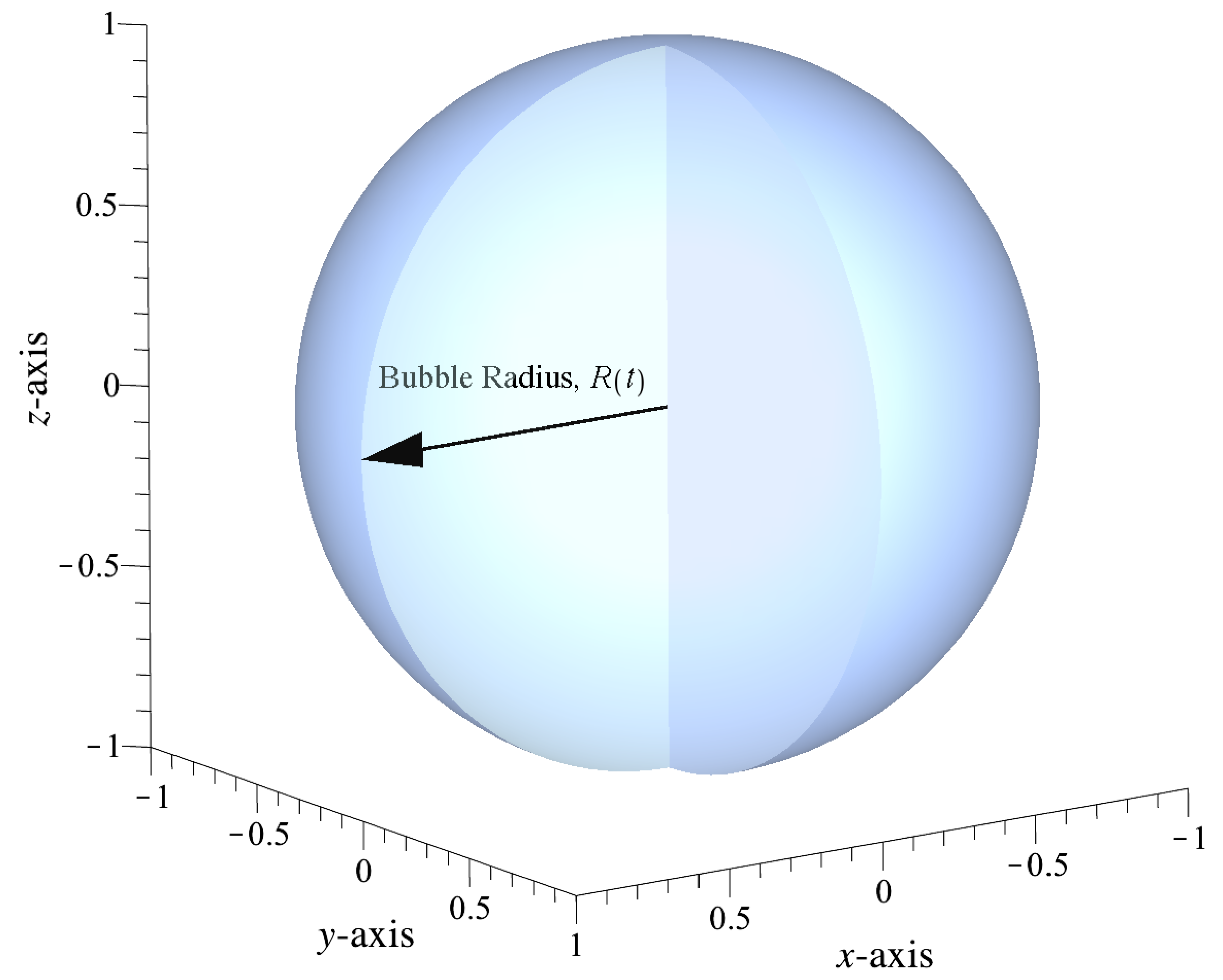
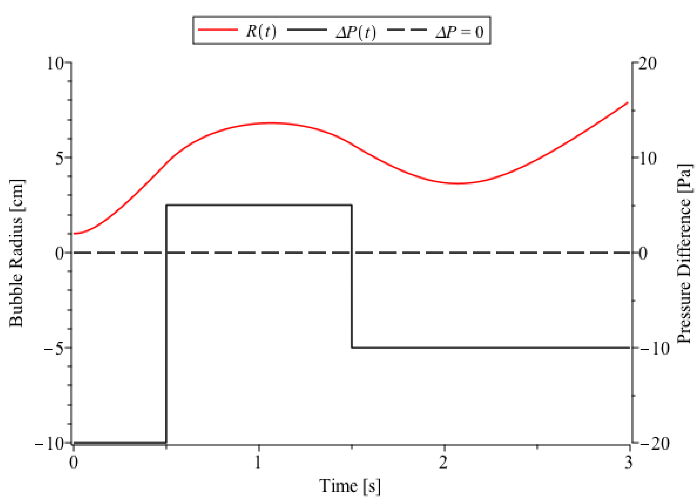
Cavitation bubble radius [m]
ρ L Surrounding liquid density [kg/m 3 ]
ν L Kinematic viscosity of surrounding liquid [m 2 /s]
γ Cavitation bubble surface tension
Δ P Cavitation bubble pressure difference
B Lagrangian energy loss proportionality constant [1/s]
Σ E Total cavitation bubble energy [J]
CMS Relevant Definitions
R Embedding of a surface Σ in R 3
Σ , . Ω Integral over a surface Σ or boundary of a solid Ω , Ω .
S , L Action S [J·s], of Lagrangian density L [J/m 2 ]
S α Surface tangent vectors, S α = α R
S α β Metric tensor on surface Σ , S α β = S α · S β
N Normal on orientable surface Σ
B α β Curvature tensor/shape operator on surface Σ . B α β = S α · β N
B α α Mean curvature, B α α = S α β B α β
CCMS-invariant normal surface speed [m/s]
˙ CMS-invariant time derivative, ˙ = t V α α
F α Surface variational stress tensor

Appendix A

δ 1 1 u z t 2 B + u z μ u z z 2 u z x 2 + 2 u z y 2 + 2 u z z 2 ρ 1 δ 1 + δ 1 1 u z t K ρ + δ 2 2 F T 1 u z u z x + 2 F T 2 u z u z y + 2 uz u z x 4 cos 4 t x 4 sin 4 t y δ + 2 uz u z y 4 sin 4 t x 4 cos 4 t y δ sin 4 t x + cos 4 t + 2 y u z x δ + cos 4 t 2 x sin 4 t y u z y δ ( 1 δ 1 ) μ ρ + A K A μ ρ 1 δ 1 + u z 2 2 u z t z + δ 3 u z u z t u z z F z + δ 3 b · ( u z F z ) + ( B + u z ) u z t u z z = 0
Setting K=A, that is,
K A = P z 2 u z z 2 = 0
this attains a solution shown below:
u z = a z P ( x , y , s , t ) d s + F 1 ( x , y , t ) ( z + a ) + F 2 ( x , y , t )
For a = π and z = π , it follows from the general solution that,
u z = π π P ( x , y , s , t ) d s + F 1 ( x , y , t ) ( z + a ) + F 2 ( x , y , t ) = F 2 ( x , y , t ) = B
due to periodicity of P on the interval [ π , π ] and the finite wall boundary condition (B) at z = π . This implies F 2 = B and thus it will be shown that the form of the solution of Equation (A1), without A K expression, is the same as the equation A = K which has a solution in Equation (A3). In the above K = P z and A = 2 u z z 2 are indeterminate forms (0/0) as δ 0 . In Equation (7) the term μ ρ 1 u z 2 ( 1 1 δ ) u z t 2 u z is expressed in terms of remaining terms in the z-component Navier-Stokes equation. The force terms are taken to be proportional to 1 δ 2 for F T and 1 δ 4 for F z . The solution of the equation without A K leads to Equation (13) when Poisson’s Equation is used. Again, the form of the solution is, u z = F 1 ( x , y , t ) H ( z ) + B .

References

  1. Fefferman, C.L. Existence and Smoothness of the Navier Stokes Equation, Millennium Prize Problems. Clay. Math. Inst. Camb. (MA) 2006, 57, 57–676. [Google Scholar]
  2. Moschandreou, T.E. No Finite Time Blowup for 3D Incompressible Navier Stokes Equations via Scaling Invariance. Math. Stat. 2021, 9, 386–393. [Google Scholar] [CrossRef]
  3. Moschandreou, T.E.; Afas, K.C. Compressible Navier-Stokes Equations in Cylindrical Passages and General Dynamics of Surfaces—(I)-Flow Structures and (II)-Analyzing Biomembranes under Static and Dynamic Conditions. Mathematics 2019, 7, 1060. [Google Scholar] [CrossRef] [Green Version]
  4. Cross, M.C.; Hohenberg, P.C. Pattern Formation outside of Equilibrium. Rev. Mod. Phys. 1993, 65, 851–1111. [Google Scholar] [CrossRef] [Green Version]
  5. Chen, Y.C.; Shi, C.; Kosterlitz, J.M.; Zhu, X.; Ao, P.; Potential, G. Topology, and Pattern Selection in a Noisy Stabilized Kuramoto-Sivashinsky Equation. Proc. Natl. Acad. Sci. USA 2020, 117, 23227–23234. [Google Scholar] [CrossRef] [PubMed]
  6. Brunet, P. The Stabilized Kuramoto-Sivashinsky Equation: A Useful Model for Secondary Instabilities and Related Dynamics of Experimental One-Dimensional Cellular Flows. Phys. Rev. E Stat. Nonlin. Soft Matter Phys. 2007, 76, 017204. [Google Scholar] [CrossRef] [PubMed] [Green Version]
  7. Zhou, J. Instability Analysis of Saddle Points by a Local Minimax Method. Math. Comput. (AMS) 2005, 74, 1–21. [Google Scholar] [CrossRef] [Green Version]
  8. He, K. Embedded Moving Saddle point and its relation to Turbulence in Fluids and Plasmas. Int. J. Mod. Phys. B 2004, 18, 1805–1843. [Google Scholar] [CrossRef]
  9. Tran, C.V.; Yu, X.; Dritschel, D.G. Velocity-pressure correlation in Navier-Stokes flows and the problem of global regularity. J. Fluid Mech. 2021, 911, A18-1–A18-18. [Google Scholar] [CrossRef]
  10. Chen, Z.-M.; Price, W.G. Time Dependent Periodic Navier-Stokes Flows on a two-Dimensional Torus. Commun. Math Phys. 1996, 179, 577–597. [Google Scholar] [CrossRef]
  11. Nelson, D.; Piran, T.; Weinberg, S. Statistical Mechanics of Membranes and Surfaces; World Scientific: Singapore, 2004; ISBN 978-981-4483-22-3. [Google Scholar]
  12. Finn, R. Capillary Surface Interfaces. Not. AMS 1999, 46, 770–781. [Google Scholar]
  13. Kudryashov, N.A.; Sinelshchikov, D.I. Analytical solutions of the Rayleigh equation for empty and gas-filled bubble. J. Phys. A Math. Theor. 2014, 47, 405202. [Google Scholar] [CrossRef] [Green Version]
  14. Pedergnana, T.; Oettinger, D.; Langlois, G.P.; Haller, G. Explicit unsteady Navier-Stokes solutions and their analysis via local vortex criteria. Phys. Fluids 2020, 32, 046603. [Google Scholar] [CrossRef] [Green Version]
  15. Alzer, H.; Ruscheweyh, S. The Arithmetic Mean—Geometric Mean Inequality for Complex Numbers. Analysis 2002, 22, 277–283. [Google Scholar] [CrossRef]
  16. Kahan, W. Notes for Math H110. Available online: https://people.eecs.berkeley.edu/~wkahan/MathH110/NORMlite.pdf (accessed on 26 June 2021).
  17. Duff, G.F.D. Navier Stokes Derivative Estimates in Three Dimensions with Boundary Values and Body Forces. Can. J. Math. 1991, 43, 1161–1212. [Google Scholar] [CrossRef]
  18. Grinfeld, P. Introduction to Tensor Analysis and the Calculus of Moving Surfaces; Springer: New York, NY, USA, 2013; ISBN 978-1-4614-7867-6. [Google Scholar]
  19. Atland, A.; Simons, B. Condensed Matter Field Theory; Cambridge University Press: Cambridge, UK, 2010; ISBN 978-0-511-78928-1. [Google Scholar]
Figure 1. Example of the periodic orbit in a cube associated with Equation (15). (a) Phase portrait of saddle-type orbit (c3 = 1280). (b) Two-dimensional set-limit cycle for c3     . (c) Visualization of Figure 1a from rotated angle. (d) Visualization of Figure 1b from rotated angle.
Applmech 02 00035 g001
Figure 2. Example of a periodic orbit in a cube. (a) Elliptical Limit Set in Oblique Coordinates. (b) Elliptical Limit Set in Lattice Cubical Cell.
Applmech 02 00035 g002
Figure 3. Schematic depicting a sphere with a time-varying radius R ( t ) . This is measured from the center of the sphere outward, and it is the primary variable of interest in a bubble process such as a Raleigh–Plesset process.
Applmech 02 00035 g003
Figure 4. Numerical Solution of the Raleigh–Plesset Equation displaying the bubble radius (red) evolving in time R ( t ) , with units [cm] on the left axis. Physical parameters were chosen to model an immersion in water: a kinematic viscosity ν L = ( 10 6 ) m 2 / s, density ρ L = ( 10 3 ) kg/m 3 , and surface tension γ = ( 7.2 · 10 2 ) N/m. A test pressure difference is also displayed, which begins at 20 Pa, then evolves to 5 Pa, and then decreases to 10 Pa, displayed against the right axis [Pa].
Applmech 02 00035 g004
Figure 5. Theorized energy loss obtained through the CMS-Lagrangian formulation of the Raleigh–Plesset equation. Here, the energy loss is assumed to be negative and is plotted on the y-axis as per the numerical solution for the bubble radius and in accordance with Equation (53) with units on the left axis. Physical parameters were chosen to model an immersion in water: a kinematic viscosity ν L = ( 10 6 ) m 2 / s, density ρ L = ( 10 3 ) kg/m 3 , and surface tension γ = ( 7.2 · 10 2 ) N/m. A test pressure difference is also displayed, which begins at 20 Pa, then evolves to 5 Pa, and then decreases to 10 Pa displayed against the right axis.
Applmech 02 00035 g005
Publisher’s Note: MDPI stays neutral with regard to jurisdictional claims in published maps and institutional affiliations.

