Article

Spherical Indentation of a Micropolar Solid: A Numerical Investigation Using the Local Point Interpolation–Boundary Element Method

Institut Jean Lamour-CNRS UMR 7198—Université de Lorraine, 2 Allée André Guinier-BP 50840, CEDEX, 54011 Nancy, France
*
Author to whom correspondence should be addressed.
Appl. Mech. 2021, 2(3), 581-590; https://doi.org/10.3390/applmech2030033
Submission received: 21 June 2021 / Revised: 14 August 2021 / Accepted: 17 August 2021 / Published: 21 August 2021
(This article belongs to the Special Issue Mechanics and Control using Fractional Calculus)

Abstract

:
The load-penetration curve in elastic nanoindentation of an elastic micropolar flat by a diamond spherical punch is analyzed. The presented results are obtained by a specifically developed numerical tool based on a judicious combination of the conventional boundary element method and strong form local point interpolation method. The results show that the usual linear relationship between the material depression and the square of the radius of the contact area is also valid in this case of micropolar elastic material. It is also shown that the relation between the indentation stress (applied load over the contact surface) and the indentation strain (ratio of contact radius by the punch radius) is linear. The proportionality coefficient which is none other than the indentation stiffness varies with the coupling factor of the micropolar elastic medium. A relation between the indentation stiffness of a micropolar solid and that of a conventional solid with the same Young modulus and Poisson ratio is derived.

1. Introduction

Depth sensing indentation is commonly adopted for the determination of local elastic and plastic properties of small size samples. In the case of homogeneous and isotropic classical elastic materials deformed at small strain, the determination of the resolved elastic modulus follows a well established analytical solution of the normal compression of two smooth solids (see, e.g., Sneddon [1], K.L Johnson [2], for example). One of the useful results relates the applied load to the relative approach of the two solids or the material depression (if one of the solids is rigid). The load and the penetration are the only quantities recorded during the test. In the classical theory, the depression is also related to the radius of the projected contact area and the radius of the spherical punch. It has been shown that, in the small strain deformation regime, the useful relation between the material depression and the radius of the contact area remains valid in the plastic regime [3].
It is more and more evident that a finer description of the mechanical behavior of some material should take into account their microstructure. This can be done in the framework of generalized continuum theories which extend the conventional continuum mechanics for incorporating intrinsic microstructural effects in the mechanical behavior of materials. Amongst the various approaches, there is the so-called micromorphic medium of Eringen [4] which is widely accepted as the most successful phenomenological top-down approach. In this theory, the impact of the microstructure of the medium is expressed at the macroscopic scale through an incompatible microdeformation tensor. The latter can be specialized depending on the prominent microscopic effect at the macro scale. Accordingly, if the prominent microscopic effect is the individual rigid rotation of the material points, the microdeformation tensor is specialized to represent this micro-rotation. The corresponding theory is that of micropolar materials also known as Cosserat materials [5]. The model was applied to porous and granular media (e.g., [6] (Ehlers, 1997) [7,8]) and even to living tissues such as bones (e.g., [9,10,11,12,13]). The identification of the material parameters of the micropolar elastic model has also been the subject of a number of works (see e.g., [14,15]. Depth sensing indentation is, among others, a valuable experimental tool for the mechanical characterization of some of this materials. The question arises as to whether the well-known relationships for homogeneous and isotropic materials remain valid in the case of elastic isotropic Cosserat materials.
The present numerical study intends to shed some light on this point. The numerical studies consider a diamond punch indenting a micropolar medium. The analysis uses the identified engineering parameters for micropolar elasticity, namely: E (the Young modulus), G (the shear modulus), ν (the Poisson ratio), l t (the characteristic length in torsion), l b (the characteristic length in bending), χ (the polar ratio), and N (the coupling number).
The specifically developed numerical tool combines the advantages of the boundary elements method and a strong form point collocation method. The method called Local point interpolation-boundary element method has been initiated by Kouitat [16] in the context of anisotropic materials. It has since proved efficient for various fields including micropolar materials (see [17,18,19]).
The governing equations of micropolar media are recalled in Section 2 below. The main steps of the LPI-BEM and the global flowchart of the numerical tool are presented in Section 3. The numerical results are shown and discussed in Section 4.

2. Governing Equations

In the theory of micropolar medium occupying the domain Ω with boundary Γ , the material point x is attached to a triad of directors that can rotate and stretch. The material point possesses six degrees of freedom: the three components of the traditional displacement vector u and the three components of a microrotation vector φ . The field equations governing this type of medium when under quasi-static evolution without external body loads are ([20,21]):
σ j i , j ( x ) = 0
m j i , j ( x ) + ϵ i j k   σ j k ( x ) = 0
In these equations, σ represents the force stress tensor and m the couple stress tensor. Next, the case of a quasi-homogeneous and isotropic solid is considered, producing the following corresponding constitutive relations:
σ i j ( x ) = λ   ε r r δ i j + 2 μ   ε i j + κ   u j , i κ   ϵ i j k φ k
m i j = α   ω r r δ i j + ( β + γ ) ω i j + ( β γ )   ω ¯ i j
ε i j = ( u i , j + u j , i ) / 2
ω i j = ( φ i , j + φ j , i ) / 2
ω ¯ i j = ( φ i , j φ j , i ) / 2
λ and μ are the Lamé constants;   α , β , γ , and κ the micropolar constants. More precisely, α , β , and γ are rotation gradient moduli. α , ( γ + β ) / 2 and ( γ β ) / 2 are also called Cosserat twist coefficients. κ is the rotation modulus is also known as the Cosserat couple modulus. The main symbols used in the paper are grouped together in the Appendix A.
With n j as the outward normal vector on the boundary, the tractions acting at a regular point of the boundary are given by:
t i = σ j i n j   and   m i = m j i n j
The material parameters must fulfill the following constraints:
( 3 λ + 2 μ + κ ) 0 ;   2 μ + κ 0 ;   κ 0 ;   3 α + β + γ 0 ;   β + γ 0 ; γ β 0

3. Solution Method

The boundary element method has already proven highly efficient for the solution of linear problems with well-established analytical fundamental solution. The boundary integral equation method in micropolar elasticity has been proposed by Sladek and Sladek [22]. An extension of the study to microstretch media is intended, thus this formulation will not be adopted. On application of the conventional BEM in this study, with Somigliana fundamental solution, the boundary element method (BEM) loses its principal appeal, namely the reduction of the problem dimension by one, due to traditional volume cells being needed in the so-called “field boundary element method” or “domain boundary element method”. This obstacle can be overcome by a number of strategies such as the dual reciprocity method [23] or radial integration method [24], which enable the conversion of volume integrals into surface ones.
In recent years, a large number of researchers have invested in the development of so-called meshless or meshfree methods. Among the various meshless approaches, the local point interpolation method is highly appealing because it is simple to implement. This approach falls in accuracy in the presence of Neumann boundary conditions, which are almost an inevitability when solving solid mechanic problems. Liu et al. have suggested a way to circumvent this difficulty by adopting the “weak-strong-form local point interpolation” method [25]. Recently, Kouitat [16] proposed a novel strategy that combines the best elements of both the conventional BEM and local point interpolation methods. This LPI-BEM approach has proved efficient in a number of contexts including micropolar elasticity [17,19]. This method is adopted in the present study and the main steps of the approach in the context of a micropolar elasticity are recalled below.
Let ν u = λ κ 2 ( λ + μ ) , μ u = μ + κ , then one could write the force stress tensor in the form:
σ i j = 2   μ u   ν u 1 2 ν u   ε r r δ i j + 2 μ u   ε i j κ   u i , j κ   ϵ i j k φ k
Similarly, set μ w = ( β + γ ) / 2 and ν w = α 2 α + β + γ ; then, the couple stress tensor reads:
m i j = 2 μ w υ w 1 2 ν w   φ r , r δ i j + 2 μ w ω i j + ( β γ ) ( φ i , j φ j , i ) / 2
The calculations were based on the assumption that the kinematical primary variables are the sum of a complementary part and a particular term, namely: u i = u i H + u i P and φ i = φ i H + φ i P .
The complementary fields satisfied the following homogeneous equations:
  μ u   1 2 ν u   u r , r j H + μ u   u j , i i H = 0
μ w 1 2 ν w   φ r , r j H + μ w   φ j , i i H = 0
These equations which are of the Navier type were solved by the conventional boundary element method, thus producing the following systems of equations:
[ H u ]   { u H } = [ G u ]   { t H }   and   [ H φ ]   { φ H } = [ G φ ]   { m H }
where { u H } , { φ H } are vectors of nodal kinematical fields and { t H } , { m H } are the vectors of nodal traction.
The particular fields solve:
  μ u   1 2 ν u   u r , r i P + μ u u i , j j P κ   u j , i j κ   ϵ j i k φ k , j = 0
μ w 1 2 ν w   φ r , r i P + μ w   φ i , j j P + ( β γ ) ( φ j , j i φ i , j j ) 2 2 κ   φ i + κ   ϵ i j k u k , j = 0
The tractions at a regular point on the boundary are written as:
t i = t i H + t i P + δ t i   with   t i A = ( 2   μ u   ν u 1 2 ν u   ε r r A δ i j + 2 μ u ε i j A ) n j       ( A = H   o r   P ) and   δ t i = ( κ   u i , j κ   ϵ j i k φ k ) n j
m i = m i H + m i P + δ m i   with   t i A = ( 2 μ w υ w 1 2 ν w   ω r r A δ i j + 2 μ w ω i j A ) n j       ( A = H   o r   P ) and   δ m i = ( β γ ) ( φ j , i φ i , j ) n j / 2
Following this, the solution of Equations (7) and (8) were considered, using a local radial point collocation method. In this method [5], a field ω ( x ) is approximated as:
ω ( x ) = i = 1 N R i ( r ) a i + j = 1 M p j ( x ) b j
with the following constraints: i = 1 N p j ( x ) a i = 0 , j = 1 M and i = 1 N .
Here, R i ( r ) is the selected radial basis functions, N the number of nodes in the neighborhood (support domain) of point x , and M the number of monomial terms in the selected polynomial basis P j ( x ) .
Coefficients a i and b j can be determined by enforcing the approximation to be satisfied at the N centers. Following some algebraic manipulations, coefficients a i and b j are expressed in terms of the field nodal values, and the interpolation is written in the following compact form:
ω h ( x ) = [ Φ ( x ) ] { ω / L }
When adopting interpolation (12) for all kinematical fields, at a given collocation center, the following were obtained:
[ B ( ) ] T [ C u ] [ B ( ) ] [ Φ ˜ ] { u / L P } + κ [ Φ 1 ˜ ] { u / L } + κ   [ Φ 2 ˜ ] { φ / L } = { 0 } [ B ( ) ] T [ C φ ] [ B ( ) ] [ Φ ˜ ] { φ / L P } + κ   [ Φ 0 ^ ] { φ / L } + ( β γ )   [ Φ 1 ^ ] { φ / L } + κ [ Φ 3 ^ ] { u / L } = { 0 }
In the above,
{ } = ( / x / y / z ) T ,   { z } = ( z 1 z 2 z 3 ) T ,   [ B ( z ) ] = [ z 1 0 0 0 z 2 0 0 0 z 3   z 2 z 3 0 z 1 0 z 3 0 z 1 z 2 ] T
Matrix B was given in terms of vector z = ( z 1 , z 2 , z 3 ) T and matrix C was the Voigt representation of the elasticity tensor.
On collection of the above equations for all the internal collocation centers, taking the assumption that the particular integrals are identically zero at all boundary points, the following forms of systems of equations were obtained:
{ u P } = [ B u u ] { u } + [ B u φ ] { φ }
{ φ P } = [ A φ φ ] { φ } + [ B φ u ] { u }
Following a similar strategy, the tractions at the boundary points could be written in the following forms:
{ t } = { t H } + [ A K u u ] { u } + [ A K u φ ] { φ } { m } = { m H } + [ A K φ u ] { u } + [ A K φ φ ] { φ }
After conducting some algebraic manipulations, the final coupled systems of equations were of the following forms:
[ H ¯ u ]   { u } + [ H u φ ]   { φ } = [ G u ]   { t }
[ H ¯ φ ]   { φ } + [ H φ u ]   { u } = [ G φ ]   { m }
It is particularly worthy of mention that the final equations contained similar boundary primary variables and internal kinematic unknowns to those of a traditional BEM. Boundary conditions can be taken into account as in standard practice.
When the problem at hand is concerned with more than one medium, then the above equations are valid for each sub-domain. Let Γ I denote a perfectly bonded interface between body A and body B . Then, for point X A of body A and point X B of body B sharing the same geometrical location in Γ I , the following conditions must be fulfilled:
t i A + t i B = 0 ( i = 1 , 2 , 3 ) ,   u i A u i B = 0   ( i = 1 , 2 , 3 )
m i A + m i B = 0 ( i = 1 , 2 , 3 ) ,   φ i A φ i B = 0   ( i = 1 , 2 , 3 )
In the case of a non-conforming contact problem, the equations must be supplemented by the unilateral contact conditions between the contacting bodies. Focusing on the case of an elastic punch, these conditions are written only for the macro displacement and macro traction. Indeed, it is believed that it is not possible to apply micro torque at the specimen boundary. The micro torque is assumed to take zero value on all boundaries. On the boundary of the contacting body A (resp. B), a potential contact area Γ A (resp. Γ B ) is defined a priori. For a node X A of Γ A and a target node X B on Γ B , the following relations apply:
t i A + t i B = 0   ( i = 1 , 2 , 3 )
d n = u n B u n A   g 0 ,   t n B   0   and   t t B = 0
In the above relations, g 0 denotes the initial normal gap between X A of Γ A and X B on Γ B . u n A and u n B stand for the normal displacements of points A and B in the direction of the common normal, which is usually taken as that of the flat specimen. t n B is the normal traction at point B and t t B is the tangential traction. It assumed here that the contact is frictionless.
Indentation by a spherical punch is a non-conforming contact problem in the sense that, for a given load, the contact surface is not known in advance. It is then advised to solve the above coupled systems of equations incrementally. Let Δ f be the increment of the field f from the previously converged solution to the actually sought solution. Then, the incremental forms of systems (15) and (16) are:
[ H ¯ u ]   { Δ u } + [ H u φ ]   { Δ φ } = [ G u ]   { Δ t }
[ H ¯ φ ]   { Δ φ } + [ H φ u ]   { Δ u } = [ G φ ]   { Δ m }
Applying the boundary conditions as usual, accounting eventually for Equation 16, global systems of the following forms are obtained:
[ A u u ] { Y u } + [ A u φ ] { Δ φ } = { F u }  
[ A φ φ ] { Y φ } + [ A φ u ] { Δ u } = { F φ }
In the case of a non-conforming contact problem, Equation (23) must be supplemented with relations (19) and (20). The resulting system of equations is nonlinear and non-differentiable. The algorithm introduced par Christensen [26] has been adopted. The pseudo code implemented for the solution of the problem is as follows:
For the actual load increment:
1.
Set k = 0,   { Y u k } = 0 , { Δ φ k } = 0 ;
2.
Solve [ A u u ] { Y u k + 1 } + [ A u φ ] { Δ φ k } = { F u } ; ;
3.
Solve [ A φ φ ] { Y φ k + 1 } + [ A φ u ] { Δ u k + 1 } = { F φ } ;
4.
If the Y u k + 1 Y u k / Y u k + 1 > ε (a given tolerance) go to 2.

4. Numerical Results

In this work, the multi-quadrics radial basis functions are applied as follows: R i ( r ) = ( r i 2 + c 2 ) q , where r i = x x i and   c and q were known as shape parameters. Shape parameter c was taken proportionally to minimum distance d 0 , defined as the maximum value among the minimum distances in the x , y , and z directions between collocation points.
Let us focus on the elastic indentation problem. For conventional materials, a famous relation of the Hertzian theory of contact states that: δ = a 2 R , with ( δ ) the indenter depression, ( a ) the radius of the projected contact disc, and ( R ) the radius of the spherical punch. Another famous relationship of the Hertzian theory of contact is the relation between the applied load ( P ), the punch radius, and the contact radius, P = K 0   a 3 R with K 0 = 4 3   E 1 ν 2 . Knowing the value of K 0 and postulating the value of the Poisson ratio, the Young modulus can be calculated.
A part of a diamond ball with radius 100 µm is considered. The boundary of the ball piece was subdivided into 100 elements with 402 boundary nodes including 153 nodes of the potential contact area. The considered micropolar solid is a cuboid with depth 5 mm and squared cross section with size 600 µm. Its boundary was subdivided into 236 elements with 1022 boundary nodes. These latter were supplemented with 1069 internal collocation centers.
The material constants of micropolar elasticity (see Equations (3) and (4)) are related to technical material parameters that have been identified individually via experiments [6]. These material parameters are:
The Young modulus E = ( 2 μ + κ ) ( 3 λ + 2 μ + κ ) 2 λ + 2 μ + κ ;
The shear modulus G = μ + κ / 2 ;
The Poisson ratio ν = λ 2 λ + 2 μ + κ ;
The characteristic length in torsion l t = β + γ 2 μ + κ ;
The characteristic length in bending l b = γ 2 ( 2 μ + κ ) ;
The polar ratio χ = β + γ α + β + γ ;
The coupling number N = κ 2 ( μ + κ ) .
Let us remind the reader that the values of   E , G , and ν are those that can be assessed by a simple tension test.

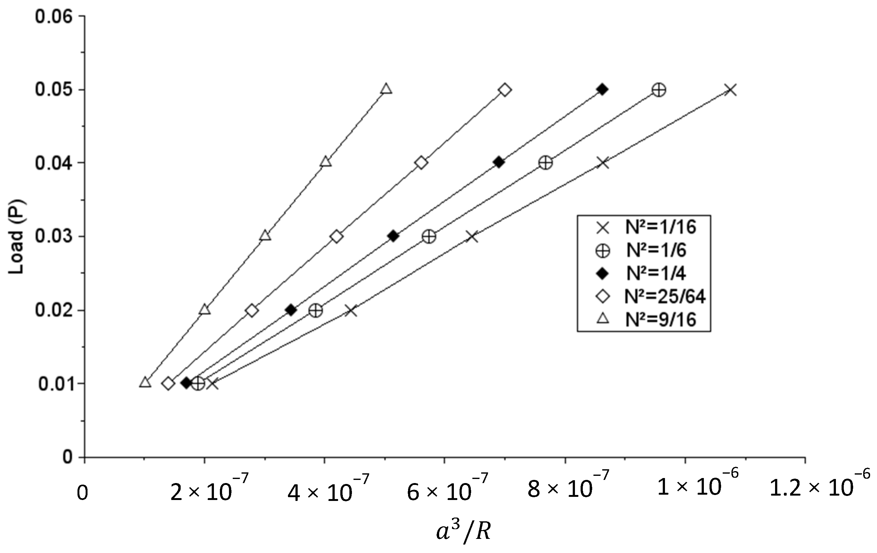
4.1. Influence of the Coupling Number

In a first set of simulation, five set of material constants were selected (see Table 1 below) leading to the following values of material parameters: E = 25,789.47     MPa , G = 8750     MPa , ν = 0.474 , l t = 0.1095     mm , l b = 0.0775     mm , and χ = 1. It should be noted that, E , G and ν have the same values for all considered cases.
As can be observed, the square of the coupling number varies from 1/16 to 9/16.
A load of 50 mN was applied on the punch in five load steps. The indenter depression ( δ ), the contact pressure distribution ( p n ), and the interval containing the contact radius ( a ) were calculated. Let R denote the radius of the spherical punch. It is found that the famous Hertzian relation  δ = a 2 R is still valid for the tested cases of micropolar solids. It is then possible to say that, having measured the punch depression and knowing its radius of curvature, the contact radius can be reached.
In Figure 1 below, the plots of P versus a 3 R are shown for the considered material parameters. It can be observed that all the curves are linear. A simple linear fit then allowed to determine the parameters of the fitting lines. The results are collected in Table 2 below.
It should be noted that, according to Hertzian theory of contact, for the given values of Young modulus and Poisson ratio, the slope of the fitting line should be K 0 = 44,333.33   MPa . It is clear from data in Table 2 that a relation of the form P = K N   a 3 R is still valid (index N is introduced to represent the coupling number). However, the value of the parameter K N varies with the coupling number.
The ratios of the calculated K N over K 0 are collected in Table 3 below.

4.2. Influence of the Characteristic Length in Torsion and the Polar Ratio

Other sets of material constants were adopted (see Table 4). They led to the same coupling numbers as in the former case. Now, l t = 0.1342 and χ = 1.5.
The values obtained for K N were those of Table 2. This means that the results are not disturbed by parameters l t and χ .

4.3. Influence of the Characteristic Length in Bending

Let us now consider the potential effect of the characteristic length in bending. For this purpose, the material parameters in Table 5 are adopted.
The characteristic length in torsion is that of the preceding case. Now, l b = 0.1095 and χ = 0.75.
Once more, the results of the calculation show that values of K N are still those in the table.

5. Conclusions

This paper concerns the numerical simulation of elastic indentation of a sphere into a flat micropolar elastic specimen. First, details of specifically developed numerical tool are given. Then, it is shown that the relation δ = a 2 R , extremely useful for direct computation of the real contact area as a function on the depression δ is equally valid for a micropolar elastic medium. It was then possible to plot the load (P) as a function of a 3 R . It then appears that a relation of the Hertzian type P = K N   a 3 R remains valid. The coefficient K N increases with the value of the coupling number N and is unaltered by other micropolar parameters, namely the characteristic lengths and the polar ratio. It is also found that K N K 0 1 N 2 where K 0 is the corresponding value as given by the Hertzian theory of contact. In conclusion, the only technical parameter affecting the indentation response of a micropolar medium is the coupling number.
Suppose that the values of parameters E , G , and ν have been obtained by a simple tension test. Then, the value of K 0 can be calculated. Knowing K 0 , one can determine the coupling number N and hence the Cosserat couple modulus κ .
Further studies are needed to allow identification of the other parameters of the model.

Author Contributions

Resources, M.T. and R.K.N.; Software, G.P., R.K.N.; funding acquisition and project supervision, P.B. and R.K.N.; writing—original draft preparation, G.P.; writing—review and editing, G.P. and R.K.N. All authors have read and agreed to the published version of the manuscript.

Funding

This research was partly funded by the IMPLANT operation (Positive Medical Personalized innovants Implantables) co-financed by the European Union through ERDF-ESF Operational “Programme Lorraine et Massif des Vosges 2014–2020”.

Conflicts of Interest

The authors declare no conflict of interest. The funders had no part in the design of the study; in the production, evaluation, or interpretation of results; in the drafting of the manuscript or the final decision to publish the data.

Appendix A

List of notations
σ j i Non symmetric macro stress tensor
m j i Couple stress tensor
u i Macro displacement vector
φ i Micro rotation vector
u i , j Displacement gradient tensor
ε i j Small strain tensor
φ i , j Micro rotation gradient tensor
ω i j Symmetric part of φ i , j
ω ¯ i j Anti-symmetric part of φ i , j
t i Traction vector
m i Micro torque vector
λ Lamé coefficient
μ Lamé coefficient
κ Cosserat couple modulus
α ,   β ,   γ Rotation gradient moduli
δ Material depression
a Radius of the projected contact area
R Radius of the indenter
P Applied load
E Young modulus
G Shear modulus
ν Poisson ratio
l t Characteristic length in torsion
l b Characteristic length in bending
χ Polar ratio
N Coupling number
K N Contact stiffness

References

  1. Sneddon, I.N. Fourier Transforms; McGraw-Hill: New York, NY, USA, 1951. [Google Scholar]
  2. Johnson, K.L. Contact mechanics, 9th ed.; Cambridge University Press: Cambridge, UK, 2003. [Google Scholar]
  3. Oumarou, N.; Jehl, J.P.; Kouitat, R.; Stempfle, P. On the variation of mechanical parameters obtained from spherical depth sensing indentation. Int. J. Surf. Sci. Eng. 2010, 4, 416. [Google Scholar] [CrossRef]
  4. Eringen, A.C.; Suhubi, E.S. Nonlinear theory of simple micro-elastic solids—I. Int. J. Eng. Sci. 1964, 2, 189–203. [Google Scholar] [CrossRef]
  5. Cosserat, E.; Cosserat, F. Théorie Des Corps Déformables; Herman et Fils: Paris, France, 1909. [Google Scholar]
  6. Lakes, R.S. Experimental microelasticity of two porous solids. Int. J. Solids Struct. 1986, 22, 55–63. [Google Scholar] [CrossRef]
  7. Diebels, S. Micropolar mixture models on the basis of the Theory of Porous Media. In Porous Media; Ehlers, P.D.-I.W., Bluhm, P.D.D.-I.J., Eds.; Springer: Berlin/Heidelberg, Germany, 2002; pp. 121–145. [Google Scholar] [CrossRef]
  8. Goddard, J.D. From Granular Matter to Generalized Continuum. In Mathematical Models of Granular Matter; Capriz, G., Mariano, P.M., Giovine, P., Eds.; Springer: Berlin/Heidelberg, Germany, 2008; pp. 1–22. [Google Scholar] [CrossRef] [Green Version]
  9. Park, H.C.; Lakes, R.S. Cosserat micromechanics of human bone: Strain redistribution by a hydration sensitive constituent. J. Biomech. 1986, 19, 385–397. [Google Scholar] [CrossRef]
  10. Cowin, S.C. Bone poroelasticity. J. Biomech. 1999, 32, 217–238. [Google Scholar] [CrossRef]
  11. Rosenberg, J.; Cimrman, R. Microcontinuum approach in biomechanical modelling. Math. Comput. Simul. 2003, 61, 249–260. [Google Scholar] [CrossRef]
  12. Ramtani, S. Electro-mechanics of bone remodelling. Int. J. Eng. Sci. 2008, 46, 1173–1182. [Google Scholar] [CrossRef]
  13. Eringen, A.C. Electromagnetic theory of microstretch elasticity and bone modelling. Int. J. Eng. Sci. 2004, 42, 231–242. [Google Scholar] [CrossRef]
  14. Diebels, S.; Geringer, A. Micromechanical and macromechanical modelling of foams: Identification of Cosserat parameters: Micromechanical and macromechanical modelling of foams. ZAMM-Journal of Applied Mathematics and Mechanics/Zeitschrift für Angewandte Mathematik und Mechanik 2014, 94, 414–420. [Google Scholar] [CrossRef]
  15. Neff, P.; Jeong, J.; Fischle, A. Stable identification of linear isotropic Cosserat parameters: Bounded stiffness in bending and torsion implies conformal invariance of curvature. Acta Mech. 2010, 211, 237–249. [Google Scholar] [CrossRef]
  16. Njiwa, R.K. Isotropic-BEM coupled with a local point interpolation method for the solution of 3D-anisotropic elasticity problems. Eng. Anal. Bound. Elem. 2011, 35, 611–615. [Google Scholar] [CrossRef]
  17. Pierson, G.; Bravetti, P.; Njiwa, R.K. Interaction implant-bone as a micropolar elastic medium: Porosity impact of the hard living media. Int. J. Theor. Appl. Multiscale Mech. 2020, 3, 229. [Google Scholar] [CrossRef]
  18. Njiwa, R.K.; Pierson, G.; Voignier, A. Coupling BEM and the Local Point Interpolation for the Solution of Anisotropic Elastic Nonlinear, Multi-Physics and Multi-Fields Problems. Int. J. Comput. Methods 2019, 17, 1950067. [Google Scholar] [CrossRef]
  19. Pierson, G.; Kouitat-Njiwa, R.; Bravetti, P. A boundary elements only solution method for 3D micropolar elasticity. Eng. Anal. Bound. Elem. 2021, 123, 84–92. [Google Scholar] [CrossRef]
  20. Eringen, A.C. Microcontinuum Field Theories; Springer: New York, NY, USA, 1999. [Google Scholar] [CrossRef]
  21. Iesan, D.; Pompei, A. On the equilibrium theory of microstretch elastic solids. Int. J. Eng. Sci. 1995, 33, 399–410. [Google Scholar] [CrossRef]
  22. Sládek, V.; Sládek, J. Boundary integral equation method in micropolar elasticity. Appl. Math. Model. 1983, 7, 433–440. [Google Scholar] [CrossRef] [Green Version]
  23. Nardini, D.; Brebbia, C.A. A new approach to free vibration analysis using boundary elements. Appl. Math. Model. 1983, 7, 157–162. [Google Scholar] [CrossRef]
  24. Gao, X.-W. The radial integration method for evaluation of domain integrals with boundary-only discretization. Eng. Anal. Bound. Elem. 2002, 26, 905–916. [Google Scholar] [CrossRef]
  25. Liu, G.R.; Gu, Y.T. A local radial point interpolation method (LRPIM) for free vibration analyses of 2-D solids. J. Sound Vib. 2001, 246, 29–46. [Google Scholar] [CrossRef] [Green Version]
  26. Christensen, P.W. A semi-smooth Newton method for elasto-plastic contact problems. Int. J. Solids Struct. 2002, 39, 2323–2341. [Google Scholar] [CrossRef]
Figure 1. Plots of load (P) versus (a3/R) for different values of the coupling number N².
Applmech 02 00033 g001
Table 1. Micropolar material constants adopted for the study of the influence of the coupling number.
λ (MPa) μ (MPa) κ (MPa) α (N) β (N) γ (N) N 2
157,5008166.671166.67002101/16
157,50070003500002101/6
157,5005833.335833.33002101/4
157,5003141.02611,217.950021025/64
157,500−250022,500002109/16
Table 2. Parameters of the line fit of the load (P) versus (a3/R).
N 2 Equation
1 / 16 P = 46,374   a 3 R + 10 4
1 / 6 P = 52,286   a 3 R + 8   10 6
1 / 4 P = 57,780   a 3 R + 10 4
25 / 64   P = 71,325   a 3 R + 6   10 5
9/16 P = 99,582   a 3 R + 2   10 4
Table 3. Comparison of the ratios KN/K0 and 1 / ( 1 N 2 ) for different values of N .
N 2 1/161/61/425/649/16
K N / K 0 1.0461.1791.3031.6092.246
1 / ( 1 N 2 ) 1.071.21.331.642.285
The results in this table show that: K N K 0 1 N 2 .
Table 4. Micropolar material constants adopted for the case lt = 0.1342 and χ = 1.5.
λ (MPa) μ (MPa) κ (MPa) α (N) β (N) γ (N) N 2
157,5008166.671166.67−1051052101/16
157,50070003500−1051052101/6
157,5005833.335833.33−1051052101/4
157,5003141.02611,217.95−10510521025/64
157,500−250022,500−1051052109/16
Table 5. Micropolar material constants adopted for the case lb = 0.1095 and χ = 0.75.
λ (MPa) μ (MPa) κ (MPa) α (N) β (N) γ (N) N 2
157,5008166.671166.67105−1054201/16
157,50070003500105−1054201/6
157,5005833.335833.33105−1054201/4
157,5003141.02611,217.95105−10542025/64
157,500−250022,500105−1054209/16
Publisher’s Note: MDPI stays neutral with regard to jurisdictional claims in published maps and institutional affiliations.

