Abstract
Understanding the effect of thermomechanical loads during finish cutting processes, in our case hard milling, on the surface integrity of the workpiece is crucial for the creation of defined quality characteristics of high-performance components. Compared to computationally generated modifications by simulation, the measurement-based determination of material modifications can only be carried out selectively and on a point-by-point basis. In practice, however, detailed knowledge of the changes in material properties at arbitrary points of the high-performance component is of great interest. In this paper, a modification of the well-known Johnson–Cook material model using the finite element software Abaqus is presented. Special attention was paid to the kinematic hardening behavior of the used steel material. Cyclic loads are relevant for the chip formation simulation because, during milling, after each cut, the material under the surface is loaded plastically several times and not necessarily in the same direction. Therefore, in analogy, multiple bending was investigated on samples made of 42CrMo4. A pronounced Bauschinger effect was observed in the bending tests. An adaptation of the material model to the results of the bending tests was only possible to a limited extent without kinematic hardening, which is why the Johnson–Cook model was supplemented by the Armstrong–Frederick hardening approach. The modified Johnson–Cook–Armstrong–Frederick material model was developed for practical use as a VUMAT and verified by bending tests for simulation use.
1. Introduction
In the finishing of high-performance components, often hard milling, a machining operation with geometrically defined cutting edges is used to achieve the final dimensional tolerances and the desired surface roughness. Especially in the die and mold making industry, hard milling is a competitive process allowing for high production rates (material removal rates) and high surface quality while ensuring a favorable residual stress state of the workpiece surface layer.
Both the surface quality and the residual stress state of the top layer significantly influence the machining time and improve the fatigue strength, corrosion resistance and creep resistance. Thus, quality control to measure surface texture is necessary for these parts. An important criterion for the part quality is the residual stress state of the surface layer [1].
Although it is of considerable importance to generate favorable residual stress states in the workpiece surface layer, a generic knowledge-based approach to reach this goal is not available yet [2].
The presence of residual stresses in structures and components has long been recognized, but only recently have many investigations been conducted on their properties with the aim of quantifying them accurately. Generally, the presence of compressive residual stresses is beneficial and of the tensile stresses is detrimental [3,4,5]. Earlier works [6,7,8] have revealed that residual stresses result from thermal strains, elastic–plastic strains and microstructural changes generated during machining. In the case of cutting operations, all of the above factors in turn are affected by the tool geometries, the cutting conditions and the properties of the work material. One of the important properties of the work material that can significantly influence the residual stress state in the milling process is strain hardening.
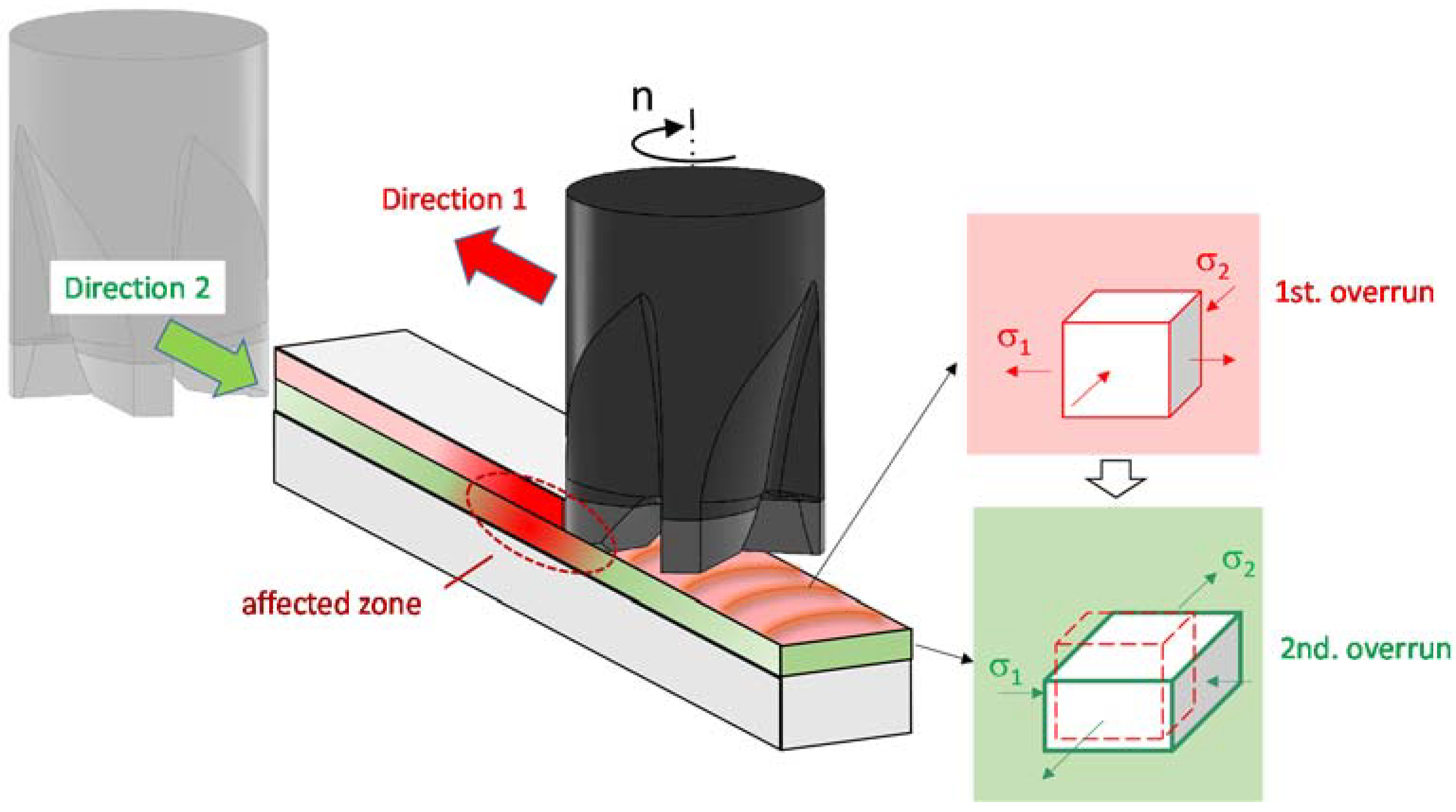
The simulations carried out so far for milling have assumed basically only one overrun, nonrepeating plastic loading of the material [9,10]. However, for a realistic description of the process, a more detailed consideration taking into account the direction of loading is desirable. The milling process generates multiple discontinuous contacts between the workpiece and the tool under changing contact conditions [2]. The successive loads occur on the one hand through individual cutting-edge engagements of the tool and on the other hand through several overruns during which the workpiece surface is machined. The workpiece zone affected by the cutter is three-dimensional and follows the tool path during machining. The dimensions of the affected zone depend on the process parameters. If the overruns have different (antiparallel) directions, a directional dependence of the hardening behavior should be taken into account (see Figure 1).

Figure 1.
Schematic representation of the milling with two overruns with the changeable directions.
This results in multiple, temporally staggered loads in different load directions, which lead to material hardening or softening. The softening depends on the number of loads and the intensity of the respective load. The cutting edge does not encounter the material in its initial state but in its changed (hardened) state. This described phenomenon is found in most polycrystalline metals. It reveals that the material’s stress–strain characteristics change as a result of the microscopic stress distribution of the material. The effect is named after the German engineer Johann Bauschinger [11].
The basis for a reliable finite element simulation is a material model that represents the mechanical properties and the behavior during machining as realistic as possible. Most engineering simulations only incorporate isotropic hardening because it is both easier to implement and to test for and usually the more dominant material behavior compared to kinematic hardening.
One of the most common material models utilized in metal cutting processes is the Johnson–Cook material model [12]. This model provides reliable results for milling materials with isotropic hardening behavior.
Previous works [13,14] have shown that the kinematic hardening models can be superior to the isotropic models in order to predict process forces and the stress state when the material undergoes cyclic loading, which leads to plastic deformations.
The investigation of kinematic hardening dates back several decades ago, when Frederik and Armstrong published one of the groundworks in this field [15].
To achieve more realistic residual stress predictions in chip formation simulations, it is of high importance to take kinematic hardening of the material into consideration. The main objective of the present work is therefore to develop a modified Johnson–Cook (JC) material model that takes into account the kinematic hardening behavior.
2. Procedure
As a modification of the isotropic or standard Johnson–Cook (SJC) material model, a coupling with the Armstrong–Frederick (AF) hardening law [15] had to be realized first. The Armstrong–Frederick hardening law adds the back stress to the JC model, which, depending on the parameterization, grows linearly in the case of monotonic deformations or saturates exponentially. In order to determine the coefficients for kinematic hardening in a coupled or modified Johnson–Cook–Armstrong–Frederick (MJC) model, bending tests were carried out on specially prepared steel samples made of quenched and tempered 42CrMo4.
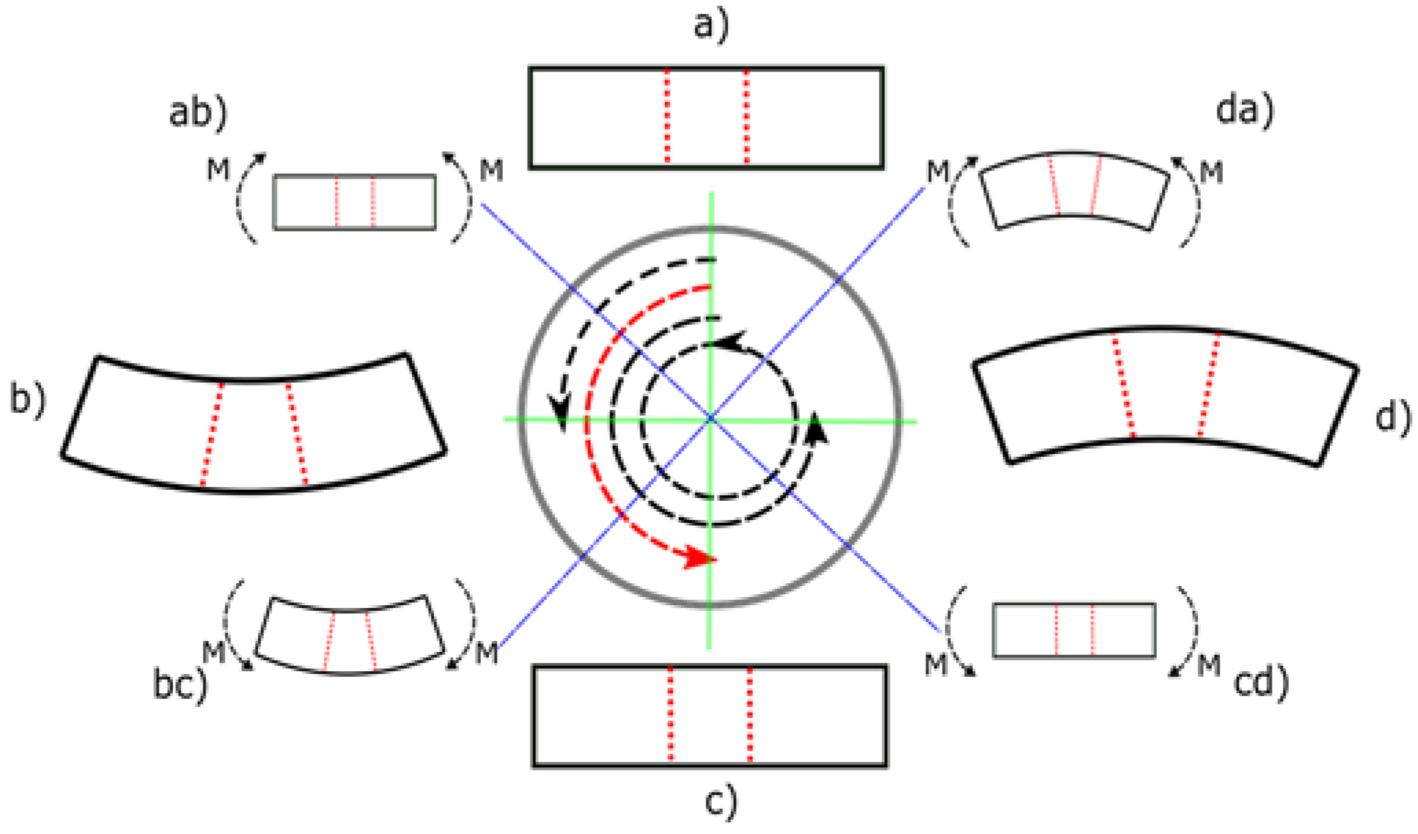
To determine the kinematic coefficient of the material, the test specimens must undergo a half cycle, i.e., they should be bent in both possible directions by the same amount of deflection.
As can be seen in Figure 2, the deformation of the test specimen was carried out in two stages, with the deformation from (a) via (ab) to (b) and (b) via (bc) to (c), each representing one phase. Both phases combined form the desired half cycle, which is represented by the red arrow in the middle. This half cycle was carried out experimentally on prepared steel samples. The material parameters were then inversely identified by finite element simulations of the bending tests. The starting point was a finished JC model whose hardening was transferred step by step to the AF portion.
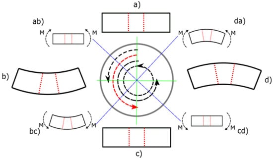
Figure 2.
Graphical representation of the cyclic deformation.
2.1. Modeling and Simulation
2.1.1. Modified Johnson–Cook Material Model
Two material models were used in the simulation, based on the Johnson–Cook material model. The Johnson–Cook model is a scalar yield stress function that depends on the accumulated plastic strain and the strain rate:
where is the reference plastic strain rate at which the A, B and n values were determined; is the accumulated plastic strain; is the plastic strain rate; A denotes the yield strength coefficient; B is the strain hardening parameter; C is the strain rate sensitivity; and n is the hardening coefficient. Here the temperature dependence that is classically part of the full Johnson–Cook model is neglected. Its parameters can be adopted to reproduce the viscoplastic part of the stress–strain curve over a wide range of temperatures, strain rates and plastic strain. However, this holds only for monotonic uniaxial tests. For application in a three-dimensional material model, one needs an equivalent stress hypothesis. Usually, the stress in Equation (1) is replaced by the von Mises equivalent stress of the deviatoric part of the Cauchy stress .
Because only the accumulated plastic strain enters in Equation (1) as an internal variable, which is insensitive to load path changes or cyclic loading, the JC model cannot cover a Bauschinger effect [16], which describes strain softening, a strength differential effect [17] or distortional hardening that changes the shape of the yield surface, such as the vertex effect [18]. Its hardening part is isotropic: the elastic range is merely inflated. The simplest way to extend the model is to shift the yield surface with respect to the stress-free state, which is referred to as kinematic hardening. To account for kinematic hardening, introducing a nonscalar internal variable is unavoidable in case of a 3D material model. This shift of the stress-free state is accounted for by a so-called back stress tensor .
Different proposals for the evolution of the back stress exist. [19] proposed to increment the back stress in direction of the plastic strain change
This linear approach allows for an infinite growth of the back stress, which is problematic when large strains occur. The approach was amended by [16] to
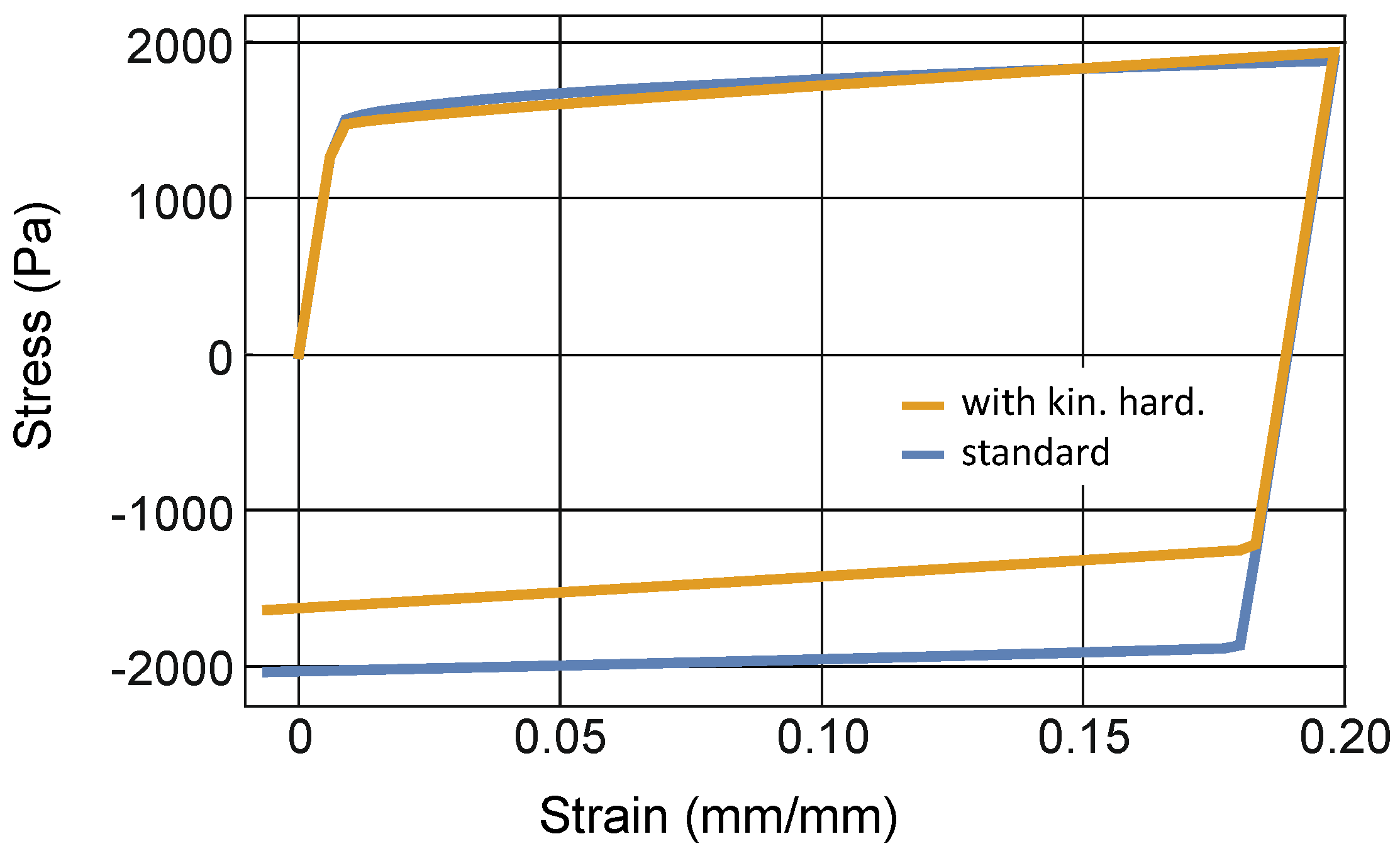
One can see that saturates exponentially towards in the direction of the strain when the loading direction is constant. While the theory is conceptually rather simple, the identification of the material parameters is difficult. In uniaxial tests with one loading direction, hardening can well be achieved by inflating or shifting the elastic range. Only upon load reversal one can see which kind of hardening prevails. However, such tests are more complicated: Reversing tensile tests into compressive tests is not feasible due to a possible buckling of the sample. Moreover, as with any plasticity theory that accounts for the loading path, the number of tests needed for identification increases dramatically. Even in the uniaxial case, the test needs to be performed for several points of load reversal. For this reason, one limits oneself to using only the linear part of the kinematic hardening law so that only one parameter has to be determined. It can be seen that this allows a reasonable adjustment of the planned tests. Figure 3 shows that already with the linear kinematic hardening, the JC model can be modified in such a way that the uniaxial load remains largely unaffected, while the load reversal part is very different between isotropic and kinematic hardening.
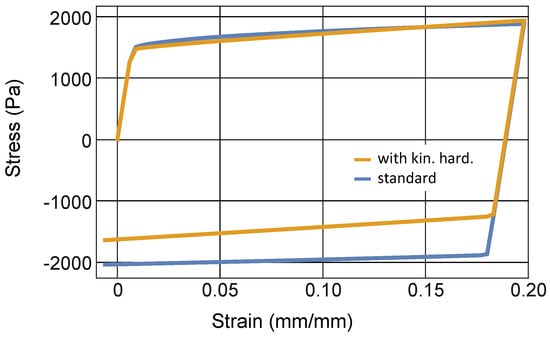
Figure 3.
Stress-strain curves in a tension-compression test up to 20% nominal strain for two parameter sets given in Table 1, one without kinematic hardening and one with a considerable kinematic hardening part.
The model parameters were defined as part of a material model already implemented in Abaqus (SJC) and for the modified Johnson–Cook model as part of an additional VUMAT code.
2.1.2. Simulation Set-Up
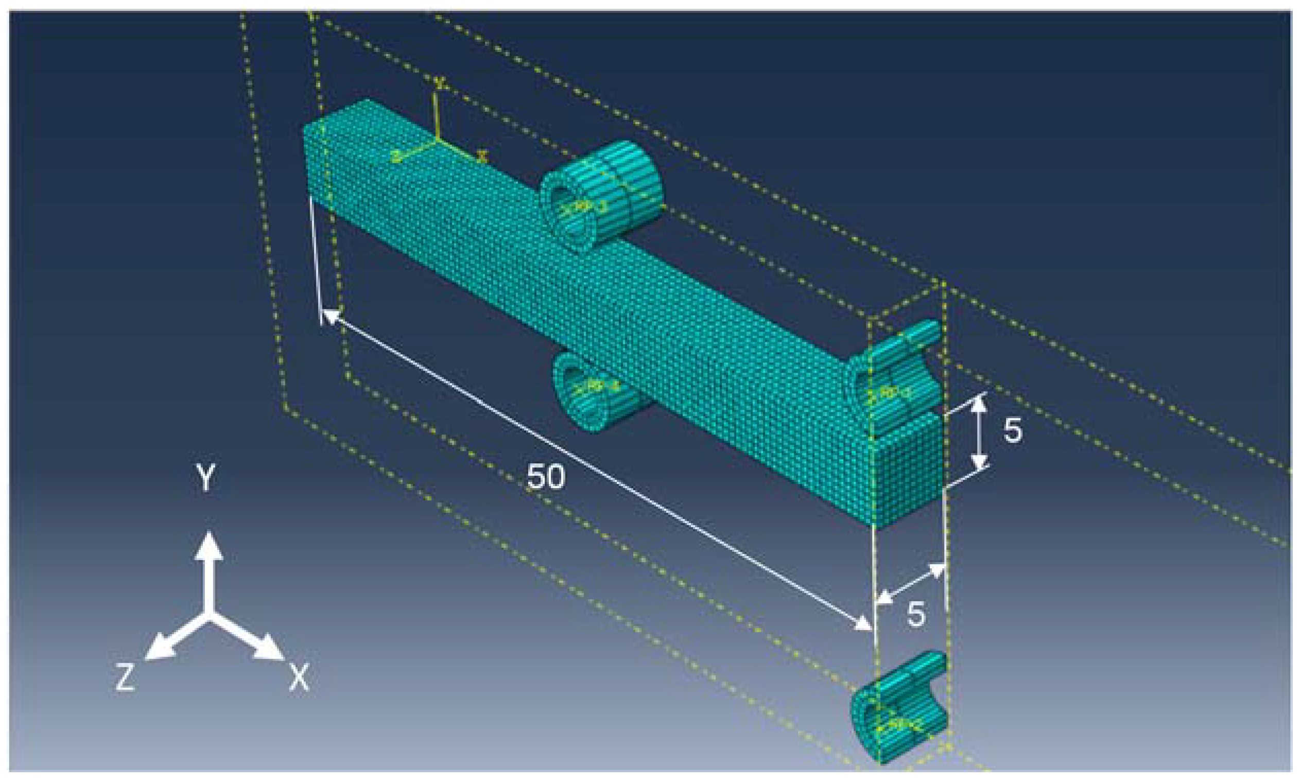
In order to reduce the computation time, a quarter of the specimen was modeled by taking advantage of the specimen’s symmetry. Instead of positioning the specimen twice, two sets of bearings were created, each consisting of two locating bearings and one fin each (see Figure 4). The bearing rollers were fixed in space, the contact of the specimen with the fin and the bearing rollers was assumed to be frictionless. In order to avoid unwanted contacts, a distance of 1 mm was created between the test body and the fin and bearings at the initial position.
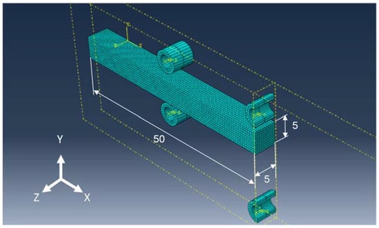
Figure 4.
Quarter symmetry design.
The bearings were defined as rigid, so they did not need a fine mesh size. On the other hand, the mesh size of the test specimen had to be finer than that of the bearings. At least five elements are required for a good stress distribution in the thickness of the test specimen. The element type (C3D8R) was selected according to the explicit solver.
2.2. Experimental Bending Tests
The test specimens consist of the steel alloy 42CrMo4 (AISI 4140) heat-treated and tempered to a hardness of 47 HRC. The test specimens were polished after heat treatment. The dimensions of the test specimens are: width: 10 mm, height: 5 mm and length: 100 mm.
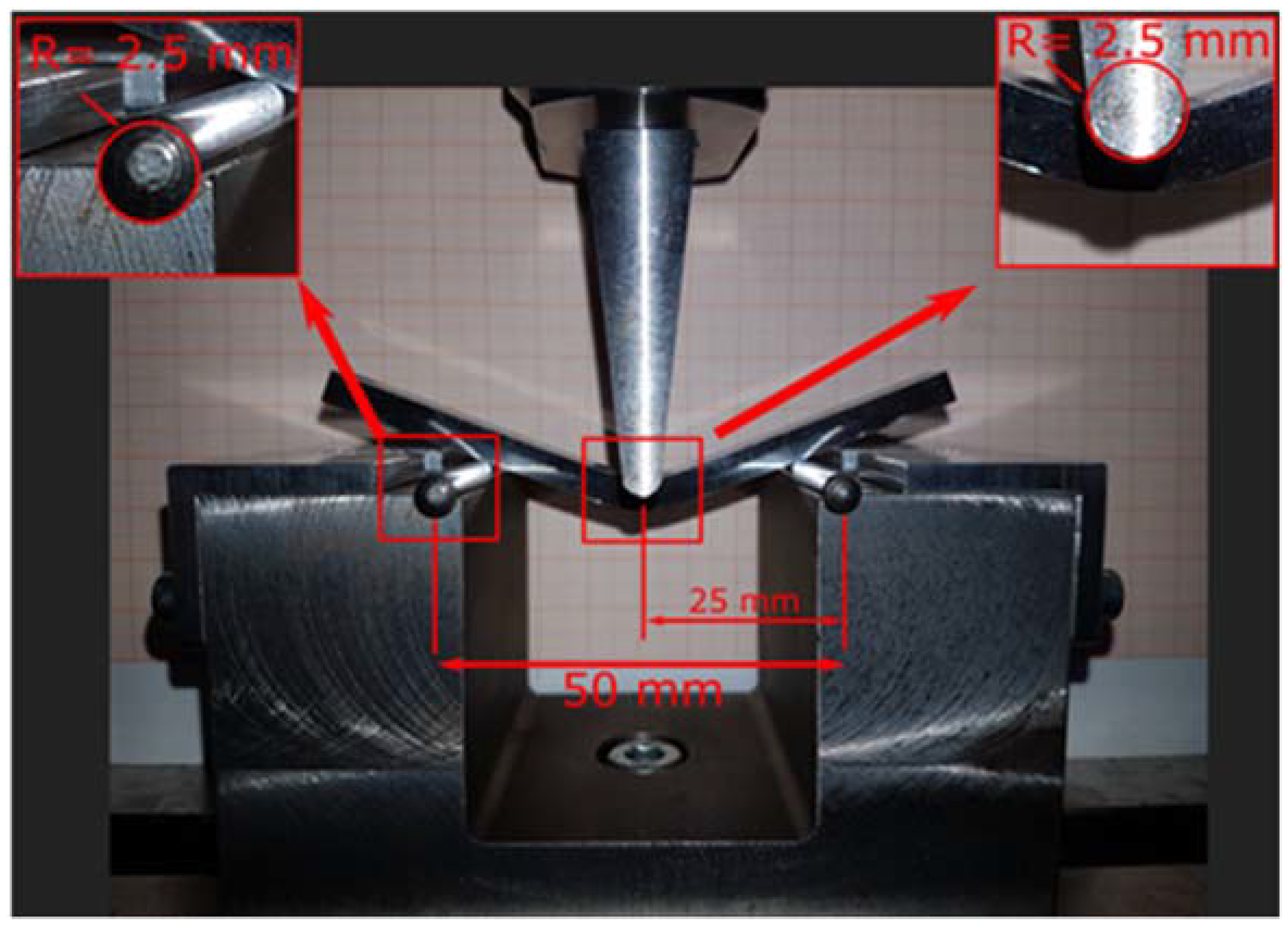
The three-point bending tests were carried out with an INSTRON SCHENCK HYDROPLUS® PSA universal device. The set-up of the three-point bending test consisted of two lower specially designed bearings (with a support span of 50 mm) and a fin placed in the middle of the support span. This set-up allowed the already deformed test specimens to be positioned stably for the second bending (see Figure 5).
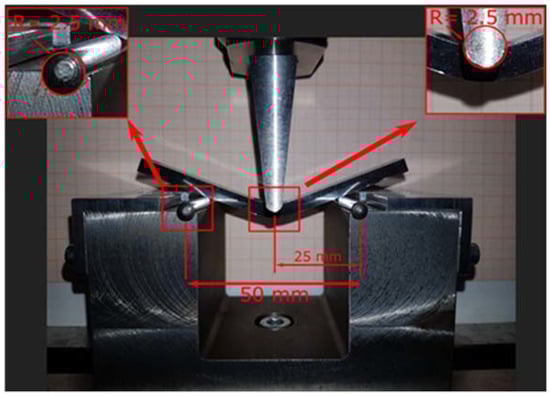
Figure 5.
Relevant dimensions of the bending device.
At the fin’s movement speed of 1 mm per minute, the machine delivered six data sets (force, displacement) per second. At the beginning, the test specimen was placed on the fixture, then the deflection was entered into the machine. The fin was moved down by the entered displacement, which bent the test specimen (see Figure 5).
The specimen was then turned over and reattached to the fixture, with the fin again manually applied to the surface of the specimen. The same displacement was entered into the machine, and the deformed specimen was deformed again.
The above procedure was repeated for different displacements (2 mm, 4 mm, 6 mm, 8 mm and 10 mm), and the force–deflection curves were obtained. All experiments were conducted at room temperature. For the validation of the simulation results with the experimental values, the extreme case with the travel distance of 10 mm was selected in this work.
3. Simulation and Experimental Results
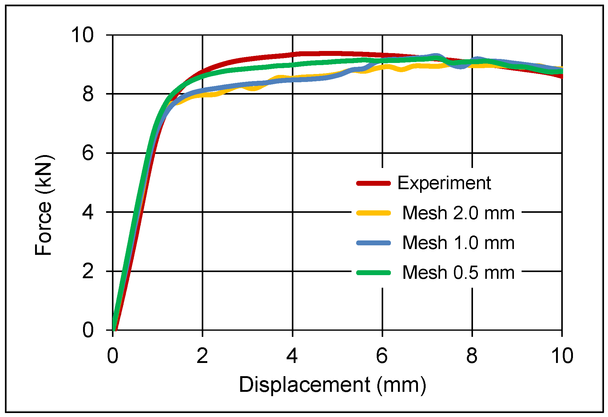
To validate the process simulation, the measured bending forces were compared with the simulation results. Due to the quarter symmetry design, the calculated forces have to be multiplied by a factor of four. The results are shown in a force–displacement (deflection) diagram for the first (see Figure 6) and the second (see Figure 7) bending when using the MJC model.
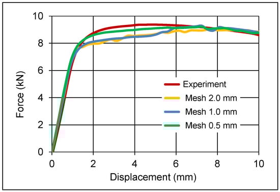
Figure 6.
Force–deflection diagram for the 1st bending test at different mesh sizes (MJC model).
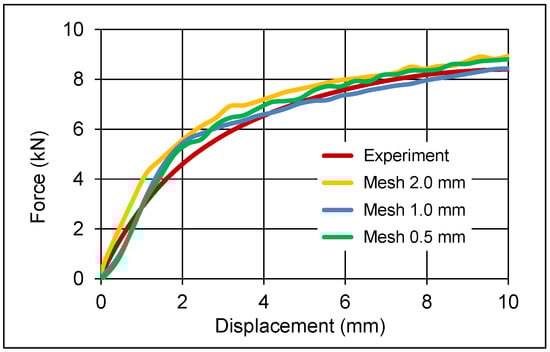
Figure 7.
Force–deflection diagram for the 2nd bending test at different mesh sizes (MJC model).
It should be noted that the mesh size of the model has a direct influence on the accuracy of the results, as shown in Figure 6 and Figure 7. The force-deflection curve tends to be closer to the experimental results with smaller mesh sizes.
Another key point is that the peaks of the force-deflection curve from the simulation of the second bending are caused by the movement of the nodes of the elements in the interface between bearing and fin (see Figure 7).
The determined force–displacement curve is shown for different displacement amplitudes in Figure 8. A clear softening can be seen with load reversal, which cannot be explained solely by the formation of a zig-zag stress profile in the flexural specimen.
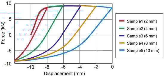
Figure 8.
Experimental force-displacement curves.
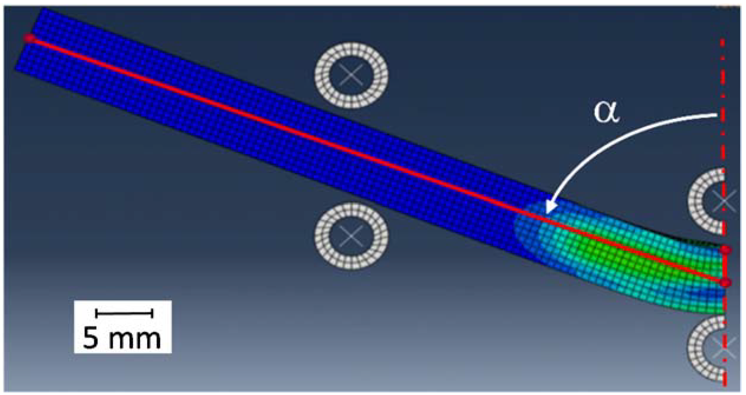
To measure the curvature from the simulation, the state is determined in the “Visualization Module” after the end of the first bending (see Figure 9). The amount of bending curvature should be doubled due to the symmetrical FE-model. If the fin moves upwards and the sample is not subjected to any external load, the angle between three points is measured and then the value is doubled.

Figure 9.
Determination of the bending curvature in the simulations.
The curvature calculated in this way is 138° compared to 140° measured in the experiment. This shows that the hardening of the material and the associated springback after free bending can be reproduced well with the MJC model.
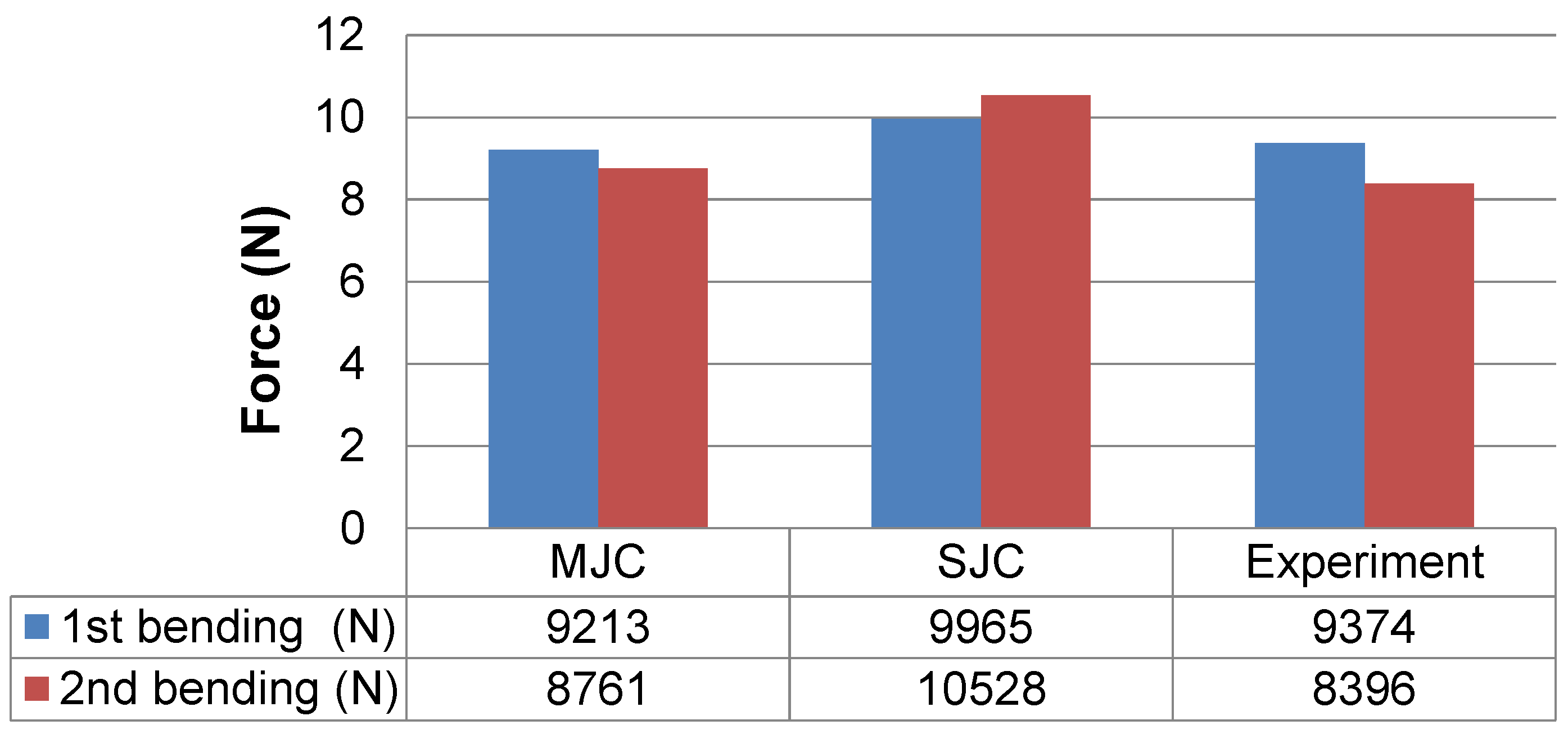
The maximum force predicted by the two models during each bending cycle is shown with the experimental data in Figure 10.
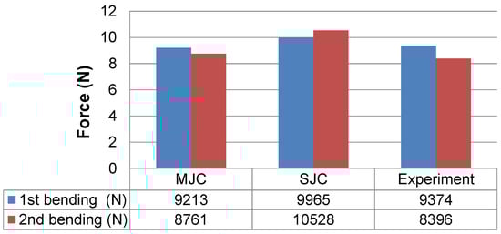
Figure 10.
Maximum force of SJC, MJC and experiment.
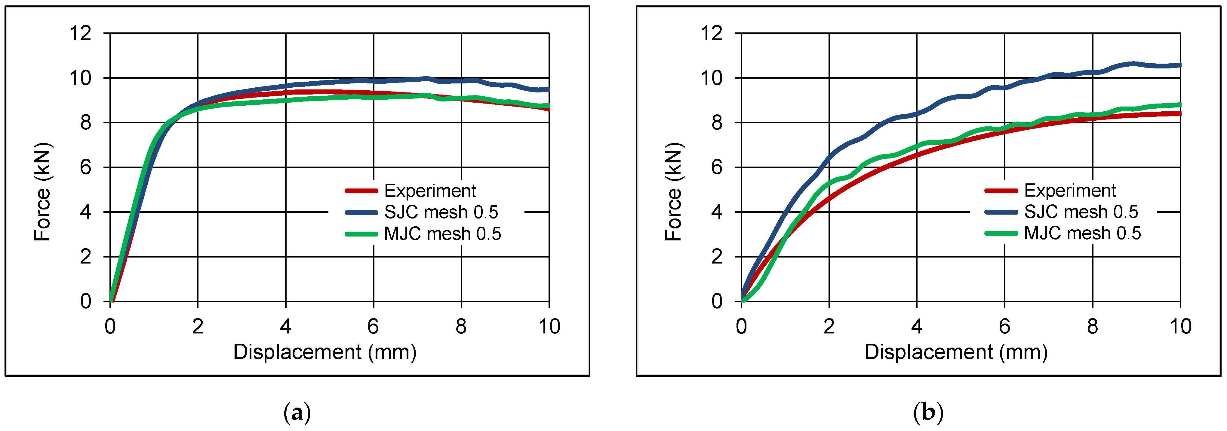
For the first bending, both models show good agreement with the experiment. However, for the reverse bending, the calculated force in the simulation according to the SJC material model is 2132 N greater than in the experiment. This overestimation results from the isotropic hardening or the missing kinematic hardening component (see Figure 11). The reason is that this simulation used the standard SJC material model, which is based on isotropic hardening. Therefore, the yield strength of the material is higher during the second bending and leads to a higher force.
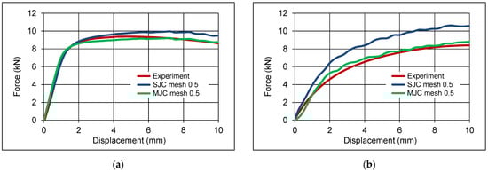
Figure 11.
Comparison of the force-deflection curve between the MJC and SJC at the (a) 1st bending and (b) 2nd bending.
The deviations between calculated and experimentally measured forces for one half cycle are shown in Table 2.

Table 2.
Accuracy of the material models for one half cycle.
4. Summary and Conclusions
Nonmonotonic deformations of the workpiece material occur regularly in various manufacturing processes. For a more accurate prediction of such processes and the resulting material properties in functionally relevant layers during the finish cutting of high-performance components, a new material model was developed. For this purpose, the standard Johnson–Cook model was extended by a kinematic strain hardening model based on the approach proposed by Armstrong and Frederick. Both the standard Johnson–Cook model and its modification with kinematic strain hardening were utilized in the simulation of a cyclic bending test. The comparison with results from experiments shows that the proposed modified Johnson–Cook model is superior to the standard Johnson–Cook model.
The comparison between the experimental data and the simulation results shows that the standard model and the modified model reproduce the first bending equally well. However, the load reversal cannot be reproduced by the standard Johnson–Cook model, as it neglects the kinematic hardening behavior of the workpiece material.
Compared to the standard Johnson–Cook model, the modified model provides more accurate values for maximum forces during bending and for a general force curve during reverse bending.
The developed modified Johnson–Cook material model is expected to provide better results for the simulation of finish machining operations of materials with pronounced kinematic hardening behavior in which nonmonotonic deformations occur.
Supplementary Materials
The following is available online at https://www.mdpi.com/2673-3161/2/3/32, Measurement data M1: Measurement data from Figure 6, Figure 7, Figure 8 and Figure 11 as recorded.
Author Contributions
Conceptualization, A.V. and R.G.; methodology, A.V. and R.G.; software, A.V.; validation, A.V., and A.P.D.; formal analysis, A.V., R.G. and A.P.D.; investigation, A.P.D. and A.V.; resources, J.S.; data curation, A.P.D. and A.V.; writing—original draft preparation, A.V.; writing—review and editing, J.S. and B.K.; visualization, A.P.D. and A.V.; supervision, J.S.; project administration, B.K.; funding acquisition, J.S. and B.K. All authors have read and agreed to the published version of the manuscript.
Funding
This research was funded by Deutsche Forschungsgemeinschaft (DFG) within the Transregional Collaborative Research Center CRC TRR 136 “Process Signatures”, project number 223500200, subproject F08. Website: http://www.prozesssignaturen.de/en/home/ (accessed on 14 August 2021).
Data Availability Statement
The data presented in this study are partially available in the supplementary materials. Additional data presented in this study are available on request from the corresponding author.
Acknowledgments
We gratefully acknowledge the Department of Mechanical Properties—IWT for performing the bending tests.
Conflicts of Interest
The authors declare no conflict of interest.
References
- Fuh, K.-H.; Wu, C.-F. A residual-stress model for the milling of aluminum alloy (2014-T6). J. Mater. Process. Technol. 1995, 51, 87–105. [Google Scholar] [CrossRef]
- Vovk, A.; Sölter, J.; Karpuschewski, B. Numerical investigation of the influence of multiple loads on material modifications during hard milling. In Proceedings of the 18th CIRP Conference on Modelling of Machining Operations, Ljubljana, Slovenia, 15–17 June 2021. [Google Scholar]
- Hosseini, E.; Holdsworth, S.R.; Kühn, I.; Mazza, E. Temperature dependent representation for Chaboche kinematic hardening model. Mater. High Temp. 2015, 32, 404–412. [Google Scholar] [CrossRef]
- Reed, E.; Viens, J. The influence of surface residual stress on fatigue limit of titanium. Trans. ASME J. Eng. Ind. 1960, 60, 76. [Google Scholar] [CrossRef]
- Bailey, J.; Jeelani, S.; Becker, S. Surface integrity in machining AISI 4340 Steel. ASME J. Eng. Ind. 1976, 98, 1007. [Google Scholar] [CrossRef]
- Khabeery, M.E.; Fattouh, M. Residual stress distribution caused by milling. Int. J. Mach. Tools Manuf. 1989, 29, 391. [Google Scholar] [CrossRef]
- Fuh, K.; Wu, C.F.; Lin, H.; Juan, H. The residual stress caused by end milling of aluminum alloy. In Proceedings of the 9th National Conference of the Chinese Society of Mechanical Engineers, Kaohsiung, Taiwan, 27–28 November 1992. [Google Scholar]
- Chou, C.H. Metal Cutting Principles; Shanghai Science Technology Press: Shanghai, China, 1984; p. 120. [Google Scholar]
- Umbrello, D.; Hua, J.; Shivpuri, R. Hardness-based flow stress and fracture models for numerical simulation of hard machining AISI 52100 bearing steel. Mater. Sci. Eng. 2004, A374, 90–100. [Google Scholar] [CrossRef]
- Uhlmann, E.; Mahnken, R.; Ivanov, I.M. Thermo-Mechanical Simulation of Hard Turning with Macroscopic Models. In Thermal Effects in Complex Machining Processes; Springer: Berlin/Heidelberg, Germany, 2018; pp. 95–132. [Google Scholar]
- Soboyejo, W. Mechanical Properties of Engineered Materials; Marcel Dekker: New York, NY, USA, 2003. [Google Scholar]
- Field, M.; Kahles, J. Review of surface integrity of machined components. CIRP Ann. Manuf. Technol. 1971, 20, 491–510. [Google Scholar]
- Taherizadeh, A.; Ghaei, A. Finite element simulation of springback for a channel draw process with drawbead using different hardening models. Int. J. Mech. Sci. 2009, 51, 314–325. [Google Scholar] [CrossRef]
- Fellmetha, A.; Zangera, F.; Schulze, V. Kinematic hardening of AISI 5120 during machining operations. Procedia CIRP 2017, 58, 104–109. [Google Scholar] [CrossRef]
- Armstrong, P.J. and Frederick, C.O. A Mathematical Representation of the Multi Axial Bauschinger Effect. Mater. High Temp. 2007, 24, 1–26. [Google Scholar]
- Bauschinger, J. Über die Veränderung der Elastizitätsgrenze und die Festigkeit des Eisens und Stahls durch Strecken und Quetschen, durch Erwärmen und Abkühlen und durch oftmals wiederholte Beanspruchungen; Mitteilungen des mechanisch-technischen Laboratoriums der Königlich Technischen Hochschule München: Berlin, Germany, 1886; Volume 13. [Google Scholar]
- Casey, J.; Jahedmotlagh, H. The Strength-Differential Effect in Plasticity. Int. J. Solids Struct. 1984, 20, 377–393. [Google Scholar] [CrossRef]
- Schurig, M.; Bertram, A.; Petryk, H. Micromechanical analysis of the development of a yield vertex in polycrystal plasticity. Acta Mech. 2007, 194, 141–158. [Google Scholar] [CrossRef]
- Prager, W.; Hodge, P. Theorie Ideal Plastischer Körper; Springer: Berlin/Heidelberg, Germany, 1954. [Google Scholar]
- Vovk, A.; Sölter, J.; Karpuschewski, B. Finite element simulations of the material loads and residual stresses in milling utilizing the CEL method. Procedia CIRP 2020, 87, 539–544. [Google Scholar] [CrossRef]
- Rech, J.; Arrazola, P.; Claudin, C.; Courbon, C.; Pusavec, F.; Kopac, J. Characterisation of friction and heat partition coeffcients at the tool-work material interface in cutting. Ann. CIRP 2013, 62, 79–82. [Google Scholar] [CrossRef]


Publisher’s Note: MDPI stays neutral with regard to jurisdictional claims in published maps and institutional affiliations. |
© 2021 by the authors. Licensee MDPI, Basel, Switzerland. This article is an open access article distributed under the terms and conditions of the Creative Commons Attribution (CC BY) license (https://creativecommons.org/licenses/by/4.0/).