Abstract
Uncertainty is a common feature in first-principles models that are widely used in various engineering problems. Uncertainty quantification (UQ) has become an essential procedure to improve the accuracy and reliability of model predictions. Polynomial chaos expansion (PCE) has been used as an efficient approach for UQ by approximating uncertainty with orthogonal polynomial basis functions of standard distributions (e.g., normal) chosen from the Askey scheme. However, uncertainty in practice may not be represented well by standard distributions. In this case, the convergence rate and accuracy of the PCE-based UQ cannot be guaranteed. Further, when models involve non-polynomial forms, the PCE-based UQ can be computationally impractical in the presence of many parametric uncertainties. To address these issues, the Gram-Schmidt (GS) orthogonalization and generalized dimension reduction method (gDRM) are integrated with the PCE in this work to deal with many parametric uncertainties that follow arbitrary distributions. The performance of the proposed method is demonstrated with three benchmark cases including two chemical engineering problems in terms of UQ accuracy and computational efficiency by comparison with available algorithms (e.g., non-intrusive PCE).
1. Introduction
Uncertainty is pervasive in science and engineering problems, for which models are widely used to study dynamic behaviors of complex systems [1]. Parameters are inputs to models, and their values cannot be exactly known due to model calibration with noisy data. Uncertainty in model parameters results in stochasticity in model outputs. Since uncertainty affects the accuracy of model predictions, it should be appropriately quantified and accounted for [2]. Such a procedure is often referred to as uncertainty quantification (UQ) [1]. The UQ has gained increasing attention for different applications, which include sensitivity analysis, parameter estimation, optimization, control, and fault detection and diagnosis [2,3,4,5,6,7,8,9,10]. For example, sensitivity assessment of arch dams was performed using a surrogate model for UQ in [9]. Besides, a numerical model for thermochemical heat storage was validated by inverse parameter estimation using Bayesian inference in [10].
Monte Carlo (MC) simulation is one of the most representative methods for UQ [11]. The implementation of MC only requires generating samples of parametric uncertainty and executing deterministic models with individual samples. Following this, the simulated results are used to calculate statistical moments of the posterior distributions of model predictions. However, MC often requires many simulations to ensure UQ accuracy, which can be computationally prohibitive.
As compared to MC, the polynomial chaos expansion (PCE) provides reliable UQ results in a computationally efficient fashion [12,13,14,15,16] and has been extensively used in various applications [4,6,16,17,18,19,20,21,22]. For instance, uncertainty in material and geometric properties of periodic structures was studied with PCE in [19,20]. In addition, uncertainty quantification in turbulent spray combustion and a rich-dome aviation gas turbine using PCE was performed in [16,21], respectively.
The PCE was first proposed in [12] based on Hermite polynomials and Gaussian random variables [13]. Later, it was extended to cover uncertainty that follows several types of probability distributions (e.g., normal and uniform), which is referred to as generalized polynomial chaos (gPC) [14]. For PCE and gPC, uncertainty is approximated by several PCE coefficients and orthogonal polynomial basis functions. While the orthogonal polynomial basis is determined depending on the type of a random variable, the PCE coefficients should be identified. For example, the coefficients of parametric uncertainty can be determined by its probability density function (PDF). However, the coefficients of model outputs are unknown and have to be calculated. Methods for calculating such PCE coefficients of model outputs are classified into intrusive and nonintrusive [23,24].
For intrusive methods, a typical approach is the stochastic Galerkin (SG) projection where the governing model is projected on each polynomial basis function through an inner product. This generates a set of coupled new models as functions of the PCE coefficients to represent the original governing model [23,24]. The main challenge of intrusive methods comes from the inner product, which generates high-dimensional integrals that are difficult to solve in real-time under many parametric uncertainties. In contrast, nonintrusive PCE [24], which is also referred to as the non-intrusive discrete projection (NIDP), can be used to calculate PCE coefficients. The implementation of NIDP is similar to MC, which generates samples to approximate uncertainty and execute the governing model with each sample. Of note, samples for non-intrusive PCE are defined as collocation points. Typically, the non-intrusive methods are computationally efficient when the number of uncertainties is small. However, the curse of dimensionality issue arises in the presence of many parametric uncertainties since the coefficients of model responses cannot be calculated in real time. To reduce the computational cost, many approaches have been developed to reduce the number of collocation points [25,26,27], while maintaining accuracy. For example, a sparse grid constructed by the Smolyak algorithm [26] was shown to be efficient, but the computational cost and the UQ accuracy are related to how the collocation points are selected [15,28].
To address these issues, we have developed an algorithm [29] to combine the generalized dimension reduction method (gDRM), namely S-variate DRM [30], with the PCE. This algorithm converts the high-dimensional integral in the inner product into several low-dimensional ones that can be easily calculated with Gaussian quadrature rules [31]. As compared to the non-intrusive methods, attempts to generate sparse collocation points in our algorithm are not required, since the total number of variables in low-dimensional integrals is small. This can save modelling efforts for UQ under many parametric uncertainties. Similar to the classic PCE (or gPC), however, our previous method only focused on uncertainty that follows standard distributions in the Askey scheme.
When uncertainty has a non-standard distribution outside the Askey scheme, the accuracy of UQ and the convergence rate can be affected. To address this, attempts were made to deal with arbitrary distributions. For instance, using the Gram-Schmidt orthogonalization [32], a Gram-Schmidt based PCE (GSPCE) was developed [33], which finds the optimal orthogonal polynomial chaos basis functions to ensure the convergence rate. In addition, other techniques, e.g., the multi-element generalized polynomial chaos [34] and the data-driven polynomial chaos expansion [35], were developed for arbitrary uncertainty. However, due to the computational cost, these algorithms were validated with either limited uncertainties or simple applications. To improve the UQ efficiency and accuracy, it is essential to develop an algorithm in the presence of many non-standard distributions of uncertainties.
The contribution of this work is to address these aforementioned issues by developing an algorithm that integrates the Gram–Schmidt (GS) orthogonalization and gDRM with the PCE to deal with a larger number of uncertainties that follow non-standard distributions. Further, to validate the performance of the algorithm, engineering examples were chosen, and the simulation results of the proposed method were compared to other popular UQ techniques (e.g., NIDP) in terms of UQ accuracy and computational cost.
This paper is structured as follows. In Section 2, a brief background of the PCE, the GS algorithm, and their integration with the gDRM is discussed, which is followed by a summary of the proposed algorithm. In Section 3, three examples are presented for algorithm verification and the conclusion is given in Section 4.
2. Mathematical Background and Methodology
2.1. Polynomial Chaos Expansion (PCE)
Suppose a stochastic model of a complex system that involves uncertain parameters and an output can be described as:
where the function defines the relationship between and . To quantify the effect of on , each element in will be approximated with the orthogonal polynomial basis and the PCE coefficients as in [24]:
where is the random variable to estimate the PDF of the uncertainty , and are the PCE coefficients of [14]. In (2), are one-dimensional orthogonal polynomials determined by the PDF of , and index is the polynomial order to accurately approximate . Since uncertainty in parameters affects model output, can be approximated with orthogonal polynomial basis and PCE coefficients as in [24]:
where are PCE coefficients of , and are multi-dimensional orthogonal polynomial basis functions determined by the tensor products of the one-dimensional polynomials for each uncertainty [12]. In (3), the index is the total number of PCE terms to approximate , which is determined by the number of parametric uncertainties and the polynomial order as in [24]:
The PCE coefficients of uncertain parameters in (2) are often determined with prior knowledge of the PDF or parameter estimation [3,24]. The unknown PCE coefficients of in (3), however, have to be calculated by substituting (2) and (3) into (1) and then by applying a spectral projection to (1) onto each polynomial basis function as defined in [24]:
where denotes the inner product, which is defined for two functions [24] as in:
where the integration in (6) is calculated over the random domain determined by , and represents a weighting function determined by the joint PDFs of [24]. Once the PCE coefficients of , i.e., are available, the mean and variance of can be quickly calculated as discussed in [24].
2.2. Techniques to Deal with Arbitrary Uncertainty
The PCE approximations as in (2) and (3) are constructed with orthogonal polynomial basis functions in the Askey scheme, which may lead to a lower convergence rate for UQ in the presence of arbitrary uncertainty. To address this, the Gram-Schmidt (GS) orthogonalization [32] was previously coupled with PCE to find the orthogonal basis via recursive procedures [33,36], which will be used in this work and hereafter referred to as GSPCE.
Once a set of one-dimensional monic orthogonal polynomials (i.e., in (2)) are defined with the GS orthogonalization, the multidimensional orthogonal polynomials (i.e., in (3)) are given by the tensor products of the one-dimensional polynomial basis [12]. These one-dimensional orthogonal polynomials are generated as in [33]:
where , and are the polynomials with the exact degree defined as . Note that the subscript of a random variable in (2) is not used to define the one-dimensional polynomial basis with the GS algorithm for simplicity. The coefficient in (7) can be given as [36]:
To calculate the inner product in (8), statistical moments of parametric uncertainty can be used. To this end, the one-dimensional orthogonal polynomial can be rewritten as in [36]:
where are the coefficients of monomial terms. The inner product between two different polynomial basis functions is defined as [36]:
where is the weighing function of the random variable and represents the raw moment of , which is defined as in [36]:
These raw moments can be calculated offline using either the functional form of the weighting function or data to form an empirical PDF. When the raw moments are available, the orthogonal polynomial basis function can be readily generated using the recursive procedure in (7). While practical and easy to implement, GS is sensitive to rounding errors and may lead to the loss of orthogonality for the resulting polynomial basis [37]. To address this issue, in this work we use the modified GS algorithm, which is numerically more stable to these errors. This algorithm will be implemented with one reorthogonalization to ensure the orthogonality of the polynomial basis [33].
To illustrate the orthogonalization step, let us define as the orthogonal polynomials (i.e., in (7)) determined by the modified GS with the reorthogonalization and set to (i.e., in (7)). Using these expressions, steps to calculate the orthogonal polynomial basis with the polynomial order are summarized in Table 1. Note that in Table 1 represents the inner product and the operator is the norm of a function. More details on the modified GS method with the reorthogonalization can be found in [37].

Table 1.
Illustration of the modified Gram-Schmidt algorithm with the reorthogonalization [37]. Reprinted from [37], Copyright (2005), with permission from Elsevier.
As compared to the PCE approximation, the exponential convergence can be obtained once the orthogonal polynomial basis functions are formulated following steps in Table 1. However, these steps can increase modelling effort since each arbitrary uncertainty should be approximated individually. It can also increase the computational cost in the presence of many parametric uncertainties. To reduce the number of uncertainties and to improve computational efficiency, two techniques in the following sections will be used in this work.
2.3. Techniques to Reduce the Number of Uncertainties
To attenuate the computational cost for UQ, the number of uncertainties can be reduced by combining a few parametric uncertainties into a similarity parameter [33]. In this work, a sampling-based approach will be used to approximate the posterior distribution of a similarity parameter characterized by an arithmetic formulation of a few parametric uncertainties. Note that the similarity parameter may have a non-standard distribution due to non-linear transformation (e.g., division and inversion). Therefore, the classic PCE cannot ensure exponential convergence and the GSPCE will be used instead. However, the GSPCE requires additional modelling effort (e.g., Mellin transform) to determine the exact PDF of uncertainty [38]. To reduce modelling effort, sampling-based approximation will be used in this work to build the empirical PDF of the similarity parameter, from which the appropriate orthogonal polynomials can be constructed with the modified GS algorithm for UQ.
For algorithm illustration, let us focus on two parametric uncertainties and and define the similarity parameter as a function of and as below:
To approximate the posterior distribution of , the first step is to randomly generate samples of and , which are defined as and , where is the total number of samples. When the PDF of each uncertainty is available, samples of and can be easily generated offline. Following this, the next step is to calculate the division with samples of and to determine the possible values of . In this way, can be defined by data points generated with samples of and , which can be defined as . Once the data points of are available, the raw moments can be evaluated as in [39]:
where is the raw moment of . Based on the raw moments of in (13), the appropriate orthogonal polynomials can be obtained following the procedures in Section 2.2.
Similarly, the procedures above can be used for other arithmetic formulations. For example, the similarity parameter that defines the inverse of the uncertainty (e.g., ) can be calculated by assuming in (12) is fixed as 1. In summary, procedures to obtain a similarity parameter with arithmetic formulation are shown in Figure 1, which will be further discussed with numerical examples in Section 3.

Figure 1.
Illustration of arithmetic formulation to derive the probability density function (PDF) of a similarity parameter.
2.4. Generalized Dimension Reduction Method
Once the orthogonal polynomials are built for parametric uncertainties, the PCE expression of the model output can be constructed with the unknown PCE coefficients as described in (3). The key to determining the PCE coefficients is to calculate a multi-dimensional integral involved in the inner product of spectral projection. Following the definition in (5) and (6), the PCE coefficients of the model output can be described as in [24]:
where is the normalization factor defined as , is the expectation operator, and is the weighting function determined by the joint PDFs of . In the presence of many parametric uncertainties (e.g., >5), the calculation of (14) can be computationally prohibitive due to the high-dimensional random space defined by . To quickly calculate high-dimensional integrals in (14), the generalized dimension reduction method (gDRM) [30] will be used, which approximates a high-dimensional integral with a few lower-dimensional ones.
Let assume a continuous and differentiable function can be defined as , which is a part of the integrand in (14). Following this, the multivariate integral in (14) can be rewritten as in:
In this way, each PCE coefficient of in (14) can be approximated with the definition of gDRM and the representation in (15) as in [28]:
where each term in is a function of random variables, which is defined as:
where , ,, , and is the mean value of the random variable (i.e., ). Further, the last term in (17), i.e., is calculated by setting all random variables to their corresponding mean values as , where . By applying the expectation operator to (17), in (16) is given as [30]:
where is the summation of a few lower-dimensional integrals to approximate in (16) and the total number of integrals is . For the last term in (16), is given as . For example, when a bivariate DMR (BiDRM) is considered, i.e., 2, the -dimensional integral in (16) is approximated with two- and one-dimensional integrals and a constant term, i.e., .
To further reduce the computational time, Gauss quadrature (GQ) rules [31,40] will be used to estimate the resulting lower-dimensional integrals in (16). For the expectation of one-variate function with a random variable (e.g., ), the one-dimensional quadrature rule can be defined as in [29]:
where is the total number of quadrature points, and is a set of quadrature points (i.e., ) and weights (i.e., ) that is used to calculate each one-dimensional integral. Importantly, quadrature rules should be selected concerning the PDFs of random variables for exponential convergence. For example, Gauss-Hermite quadrature rules are the best choice for Gaussian random variables [31]. For arbitrary variables, quadrature points and their weights can be readily identified using the orthogonal polynomial basis from the GS algorithm. Details to determine the quadrature points and their corresponding weights are summarized in Appendix A. Once the one-dimensional quadrature rules are built for individual random variables, a full tensor product grid for a multidimensional integral (i.e., ) can be constructed by using tensor products of the one-dimensional quadrature rules.
For clarity, suppose that each PCE coefficient in (16) is calculated with the BiDRM (i.e., 2). This means that an -dimensional integral (i.e., in (16)) will be approximated with one- and two-dimensional ones in total. These lower-dimensional integrals can be further calculated with the quadrature rules as below [29]:
where ( 1 and 2) is the total number of quadrature points and weights for each integration variable , and the operator denotes tensor product. Following tensor product rules, the total number of quadrature points to calculate the multivariate integrals (i.e., ) can be given as [40].
To quantify the required computational effort for BiDRM, the number of evaluations () to approximate a high-dimensional integral in (16) is defined as:
where and are the number of quadrature points to calculate two- and one-dimensional integrals, respectively. In this work, five quadrature points and their corresponding weights will be used for each random variable. Thus, and are 25 and 5, respectively. In addition, the last term, i.e., 1 in (22), represents the calculation of the constant term .
2.5. Summary of the Uncertainty Quantification (UQ) Algorithm
The UQ algorithm in this work can be summarized as follows, which integrates the modified Gram-Schmidt (GS) orthogonalization, generalized dimension reduction method (gDRM), and quadrature rules to quickly calculate the PCE coefficients of model predictions.
- Build orthogonal polynomial basis functions for parametric uncertainty that follows an arbitrary distribution using the modified GS orthogonalization.
- Determine the PCE coefficients and the polynomial basis for the PCE expression of each parametric uncertainty (e.g., and in (2)).
- Construct the multi-dimensional orthogonal polynomials (e.g., in (3)) for the model prediction (e.g., ) using tensor products of the one-dimensional polynomial basis functions.
- Construct surrogate models of model outputs with the spectral projection (e.g., in (5)), which are functions of unknown PCE coefficients of model predictions.
- Convert each high-dimensional integral in the inner product into a family of lower-dimensional ones that involve at most integration variables, using the gDRM.
- Solve these lower-dimensional integrals with Gauss quadrature (GQ) rules.
- Quantify the effect of parametric uncertainty on model outputs of a complex system using the PCE coefficients of model predictions.
3. Simulation Studies
For algorithm validation, three cases including two examples in chemical engineering were used, which involve uncertainties that follow different types of non-standard distribution. While specific examples are used in this work, our approach is transformative to other engineering problems. Note that uncertain parameters in each example are assumed to be independent and not correlated because our objective is to validate the algorithm to deal with many parametric uncertainties.
In addition, the algorithm in this work was compared with the gDRM-based UQ algorithm in the Askey scheme and other non-intrusive PCE-based algorithms. To program and execute each example with these approaches, in-house codes with MATLAB® were used and performed on an office desktop (Core i5-8400 central processing unit (CPU) at 2.80 GHz). To compare the UQ accuracy, the mean and the variance of model outputs were calculated for individual methods. Further, the relative error () of the variance was determined using the results of MC simulations, which is defined as in:
where is the reference of the variance in model outputs estimated with MC, and is the variance of model outputs obtained with different UQ algorithms.
3.1. Example 1: Algebraic Function
A model response as in (24) was first used for algorithm verification and comparison:
where is the model response, and , , and are model input variables, which are set to 1. In addition, are model parameters, and each parameter is defined as a parametric uncertainty. A 10% variation around the mean value of each parameter was introduced, and our objective is to quantify the joint effect of on . Details about are summarized in Table 2.

Table 2.
Description of parametric uncertainties in Example 1.
For comparison, three different case scenarios were considered. For the first two case studies, the modified GS algorithm with the reorthogonalization step was used to build the polynomial basis functions for uncertainties that are not considered in the Askey scheme, e.g., the Gumbel, lognormal and Weibull distributions in Table 2. In the first case study, each uncertainty was approximated with a PCE expression, which will be referred to as the GSPCE. Since there are 10 parametric uncertainties, the random space is ten-dimensional for the GSPCE. In the second case study, reconstruction of the multidimensional polynomial basis was performed to reduce the total number of uncertainties, which is referred to as the reconstructed GSPCE (rGSPCE). For rGSPCE, several parametric uncertainties in (24) were combined into a single uncertainty, following the description in Section 2.3. For example, the product between and was treated as one uncertainty and the ratio of to was defined as the second source of uncertainty. Similar operations were applied to the other two terms in (24). In this way, the random space of rGSPCE is four-dimensional. In the third case study, polynomial basis functions of standard distributions (i.e., normal) in the Askey framework were used to approximate each uncertainty, which is hereafter referred to as the ASPCE. The random space for the ASPCE is 10-dimensional.
Once the PCE expressions of parametric uncertainties are constructed with either the GS orthogonalization or the orthogonal polynomial basis functions in the Askey scheme, the PCE coefficients of can be calculated and used to quantify the impact of uncertainties on model output. To solve the PCE coefficients of in (24), the gDRM was used in all three case studies to convert high-dimensional integrals in the spectral projection as in (14) into low-dimensional ones that can be quickly solved with quadrature rules.
For algorithm illustration, the BiDRM in Section 2.4 was used in this work. As such, was set to 2 in (16), which means each high-dimensional integral in the spectral projection (e.g., the ten-dimensional integrals for the ASPCE- and the GSPCE-based UQ methods and the four-dimensional integrals for the rGSPCE algorithm) was approximated with a few one- and two-dimensional ones to calculate the PCE coefficients of . These lower-dimensional integrals were calculated with Gauss quadrature rules and details about the calculation can be found in Section 2.4 and Appendix A.
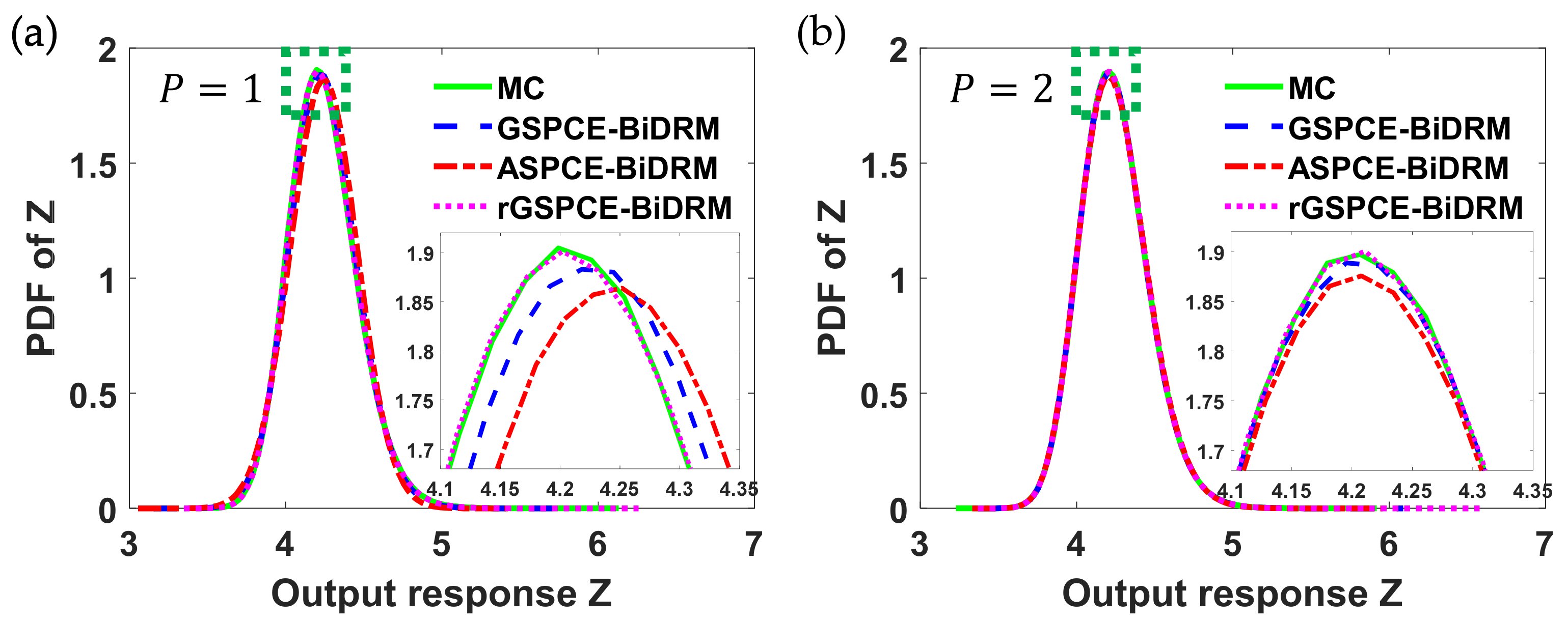
To compare the UQ accuracy in these case studies, simulations were conducted when the polynomial order ( of each parametric uncertainty was set to 0, 1, and 2, respectively. The simulation results are shown in Figure 2. For comparison, the results of MC are also given in Figure 2, for which the number of samples was set to 106 for each parametric uncertainty to ensure the UQ accuracy.
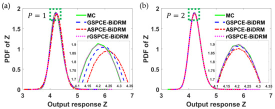
Figure 2.
Simulation results of the probability density function (PDF) of with different polynomial orders () in each case study: (a) 1 and (b) 2.
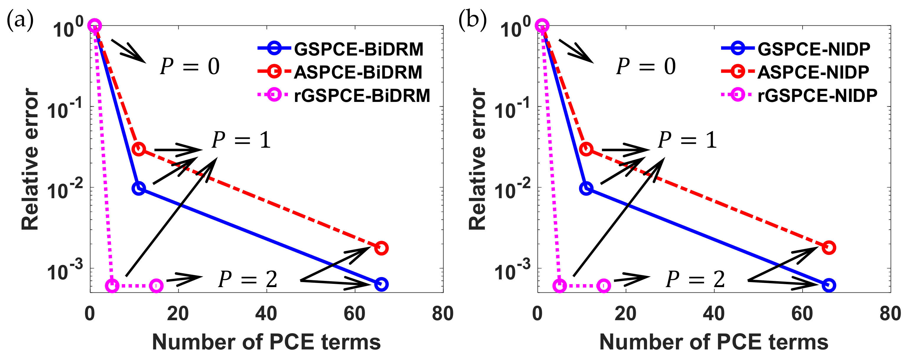
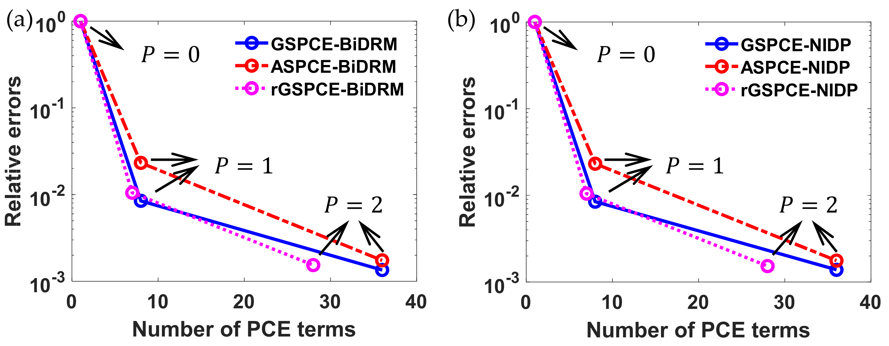
Note that when the polynomial order () of each uncertainty was set to 0, the uncertainty in cannot be quantified, since only one PCE coefficient was used to generate surrogate models of , which only consider its mean value. Thus, the PDFs of in different case studies, when was set to 0, were not included in Figure 2. As seen in Figure 2, it was found that as the polynomial order increases, the PCE-based methods converge to the results of MC. This implies that the UQ accuracy is related to the total number of polynomial terms to approximate uncertainty. To quantitatively compare UQ accuracy with respect to different polynomial orders, the relative error of the variance of was calculated in each case study using (23). The results are shown in Figure 3a. Note that once the PCE coefficients of in (24) are available, the variance can be analytically determined following steps discussed in [24].
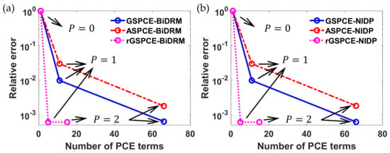
Figure 3.
Comparison of the relative error of the variance for with different (a) bivariate dimension reduction method (BiDRM)- and (b) non-intrusive discrete projection (NIDP)-based polynomial chaos expansion (PCE) approaches.
Each line in Figure 3a represents a specific case study, and three circle markers on each line show the relative errors with respect to different polynomial orders (i.e., was set to 0, 1, and 2, respectively). As seen in Figure 3a, the total number of PCE terms for in each case study is different since it is a function of the polynomial order and the total number of uncertainties . In addition, as the polynomial order increases, the relative error of the variance of decreases. Further, the GS-based PCE (i.e., GSPCE and rGSPCE) provide smaller relative errors, as compared to the ASPCE. This is because polynomial basis functions in the ASPCE are designed for standard distributions (e.g., normal) in the Askey framework, but arbitrary uncertainties (e.g., Gumbel in Table 2) are considered in this example. This clearly shows the UQ efficiency of the GS-based PCE. Moreover, as compared to the GSPCE-based method, it was found that the relative error of the rGSPCE-based method is one magnitude smaller, when was 1 (see Figure 3a). In contrast, the difference in between the GSPCE-based and the rGSPCE-based methods is insignificant, when was 2. However, it is important to note that the number of PCE terms required to approximate uncertainty in is much smaller for the rGSPCE-based method (<20). Since fewer PCE coefficients are required, it can greatly reduce the computational cost, which will be discussed below.
To further validate the efficiency of the algorithm in this work that integrates the GS and gDRM with the PCE, simulations were conducted to compare the algorithm with the full tensor product grid-based non-intrusive discrete projection (NIDP). Similar to the three case studies mentioned above, three additional case studies were investigated using the NIDP method. In the first case study, the modified GS method was used to construct the polynomial basis functions for each uncertainty, but the PCE coefficients of were solved with the NIDP. This is referred to as the GSPCE-NIDP in Figure 3b. In the second case study, reconstruction of the multidimensional polynomial basis was performed to reduce the total number of uncertainties and NIDP was used to solve the PCE coefficients of , which is referred to as the rGSPCE-NIDP. In the third case study, polynomial basis functions of standard distributions were used to estimate each parametric uncertainty, which is referred to as the ASPCE-NIDP.
The results of NIDP-based UQ are shown in Figure 3b. Details about the implementation of the NIDP approach in each case study to solve the PCE coefficients for can be found in [24]. As compared to the results in Figure 3a, it was found the relative error of the BiDRM-based approach is identical to the NIDP-based method in Figure 3b. For example, when was set to 2, the relative error of the rGSPCE-BiDRM is ~0.000607, which is identical to the rGSPCE-NIDP. As compared to the non-intrusive methods, this validates the UQ accuracy of the algorithm in this work, which uses the gDRM to approximate high-dimensional integrals in the spectral projection.
To show the performance of the algorithm in this work, we also compared the computational efficiency for each case study. Specifically, the total number of PCE coefficients of and the number of evaluations to approximate each PCE coefficient are summarized in Table 3. For the algorithm in this work, it is worth mentioning that is measured by counting the number of quadrature points to approximate each integral as defined in (22), for which the number of quadrature points in each dimension was set to 5. For example, the number of evaluations to calculate a PCE coefficient for the GSPCE- and ASPCE-BiDRM is , since there are 10 one- and 45 two-dimensional integrals resulting from the BiDRM step, i.e., . In contrast, the number of evaluations to calculate a PCE coefficient is 171 for the rGSPCE-BiDRM, since the BiDRM only generates 4 one- and 6 two-dimensional integrals, i.e., . Further, when the non-intrusive full tensor product grid-based NIDP is used, the number of evaluations to approximate a PCE coefficient of is and for the ten- and four-dimensional random space, respectively.

Table 3.
Summary of the number of PCE coefficients of and the number of evaluations to solve a PCE coefficient in Example 1. For each case study, GSPCE-BiDRM, ASPCE-BiDRM, and rGSPCE-BiDRM refer to a Gram-Schmidt based PCE, an Askey-scheme based PCE, and a reconstructed GS based PCE, coupled with bivariate dimension reduction method (BiDRM), respectively. GSPCE-NIDP, ASPCE-NIDP, and rGSPCE-NIDP are GSPCE, ASPCE, and rGSPCE, combined with the nonintrusive discrete projection (NIDP), respectively.
As seen in Table 3, the number of evaluations for the non-intrusive methods is significantly higher than the BiDRM-based methods. As discussed above, our algorithm that integrates the GSPCE (or rGSPCE) with BiDRM provides as accurate results as the nonintrusive approaches. However, it can greatly reduce the computational cost to calculate the PCE coefficients. For example, ~1.2969 s were required to solve the total PCE coefficients with the rGSPCE-NIDP, when was set to 2. In contrast, ~0.9688 s were required to estimate the PCE coefficients when the rGSPCE-BiDRM was used. Compared to the non-intrusive method, this is ~25% lower. Because the computational time for the NIDP-based methods is larger than the BiDRM-based methods, we will hereafter focus on discussing the computational efficiency of the BiDRM-based methods. The computational time in each case study is summarized in Table 4 for the BiDRM-based methods and the ASPCE-NIDP method that is considered the original PCE method.

Table 4.
Summary of the computational time to quantify uncertainty in model output in Example 1.
As can be seen in Table 4, the computational time increases as increases. It was also found that the rGSPCE-BiDRM-based method that has four-dimensional random space requires less computational time, as compared to the other two case studies. For example, when was set to 2, the time for the rGSPCE to calculate all PCE coefficients was ~0.9688 s, which is significantly lower than the ASPCE- and GSPCE-BiDRM methods. Besides, it was found that the computational time of the ASPCE-NIDP is large for each polynomial order , compared to the BiDRM-based methods, and is increased significantly as increases. This shows the advantage of our algorithm at combining the GS and BiDRM with PCE. To further validate our algorithm, two examples in chemical engineering will be followed.
3.2. Example 2: Membrane Reactor
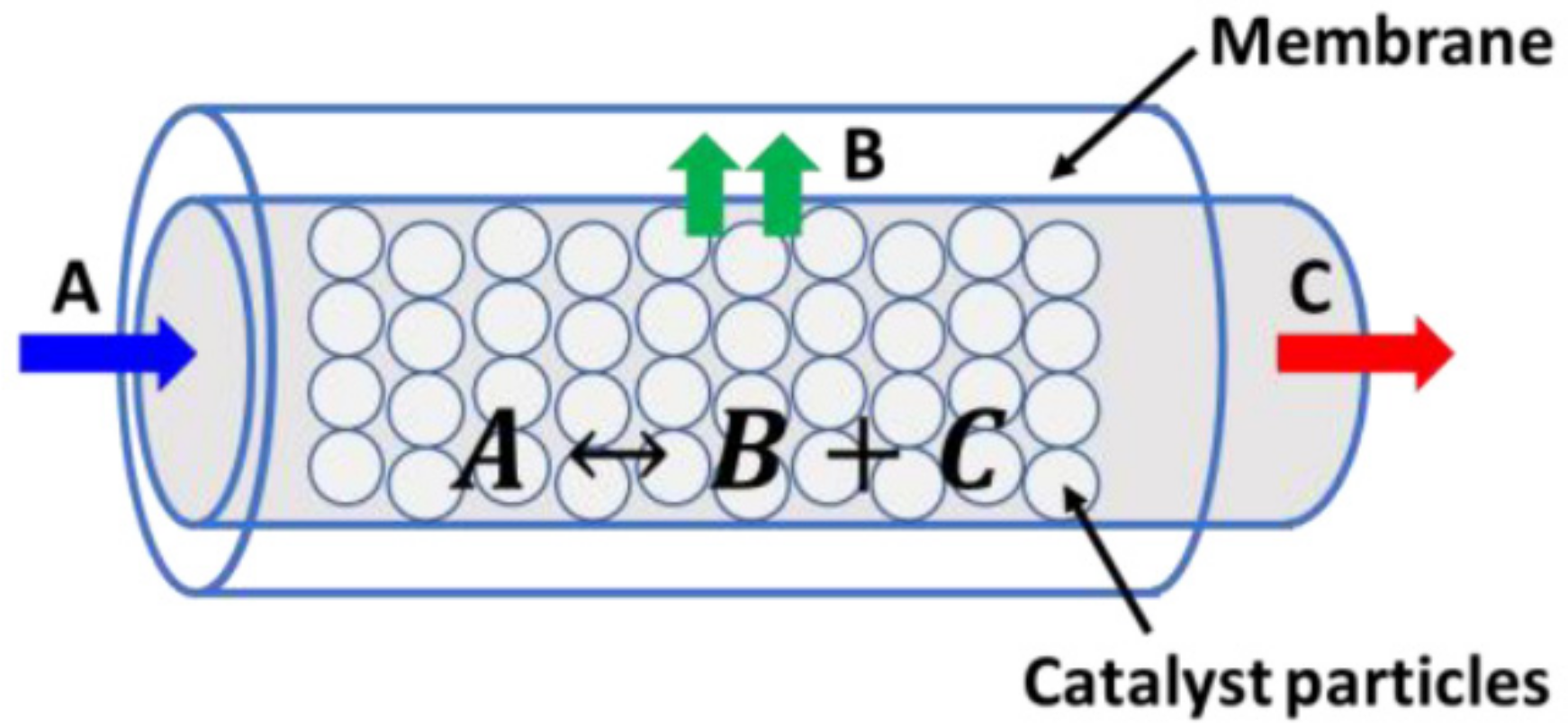
An inert membrane reactor with catalyst on the feed side (IMRCF) is shown in Figure 4, where the following reaction occurs [41,42]:

Figure 4.
Illustration of IMRCF reactor system [41,42].
In this example, the reactor is operated at the given temperature () and pressure (), and the membrane is only permeable to product B, which diffuses through the membrane with the molar flux . Following this, the mole balances of , , and can be described as in [41,42]:
where , , and are the molar flow rate of , , and , respectively, and is the reactor volume. The reaction rate law of and the molar flux of through the membrane, i.e., , are given as [41,42]:
In this example, model parameters in (29)–(31) are summarized in Table 5 and details can be found in [41,42].

Table 5.
Description of model parameters in Example 2 [42].
For algorithm validation, all parameters except the gas constant R were assumed to follow a lognormal distribution with a 10% variation around the mean of each parameter in Table 5. Since there are five uncertainties, the resulting random space is five-dimensional (). As in Example 1, three case scenarios were investigated by combining the GSPCE, ASPCE, and rGSPCE with the BiDRM, respectively. For the GSPCE- and rGSPCE-based case studies, the PCE expression of each parametric uncertainty was formulated with the modified GS. For the ASPCE-based case study, the PCE expressions for uncertain parameters were approximated with the orthogonal polynomial basis functions in the Askey scheme. Further, for the rGSPCE-based case study, the ratio between pressure and temperature in (31) were combined into one uncertainty, and the reciprocal of in (29) was treated as another source of uncertainty. These will reduce the number of uncertainties by 1, resulting in a four-dimensional random space. To calculate the PCE coefficients of model outputs in (26)–(28), the BiDRM was used in three case studies to transform high-dimensional integrals in the spectral projection into a few low-dimensional ones, which can be numerically solved with quadrature rules.
The quantification of uncertainty in the molar flow rate was chosen to compare the UQ accuracy in different case studies. In each case study, the polynomial order () of uncertainty was set to 0, 1, 2, and 3, respectively. In addition, 106 samples were used for MC to obtain the reference to calculate the relative errors as in (23). The simulation results are given in Figure 5.
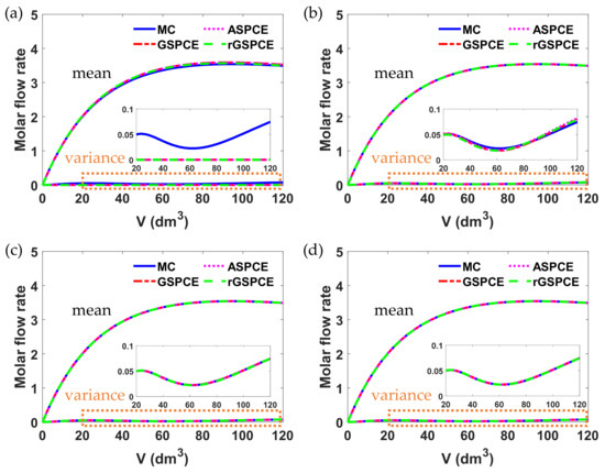
Figure 5.
Simulation results of molar flow rate with different polynomial orders () in each case study: (a) , (b) , (c) , and (d) .
As seen in Figure 5, when the polynomial order was set to 0, all case studies cannot estimate the uncertainty in model output (), since there is only one term in the PCE expression of that only considers its mean value. Thus, the effect of parametric uncertainties on model outputs cannot be quantified. Similar to Example 1, it was found that the accuracy of UQ increases as the polynomial order () increases. As seen in Figure 5c,d, all case studies have almost identical results for the mean and variance of , when was set to 2 and 3, respectively.
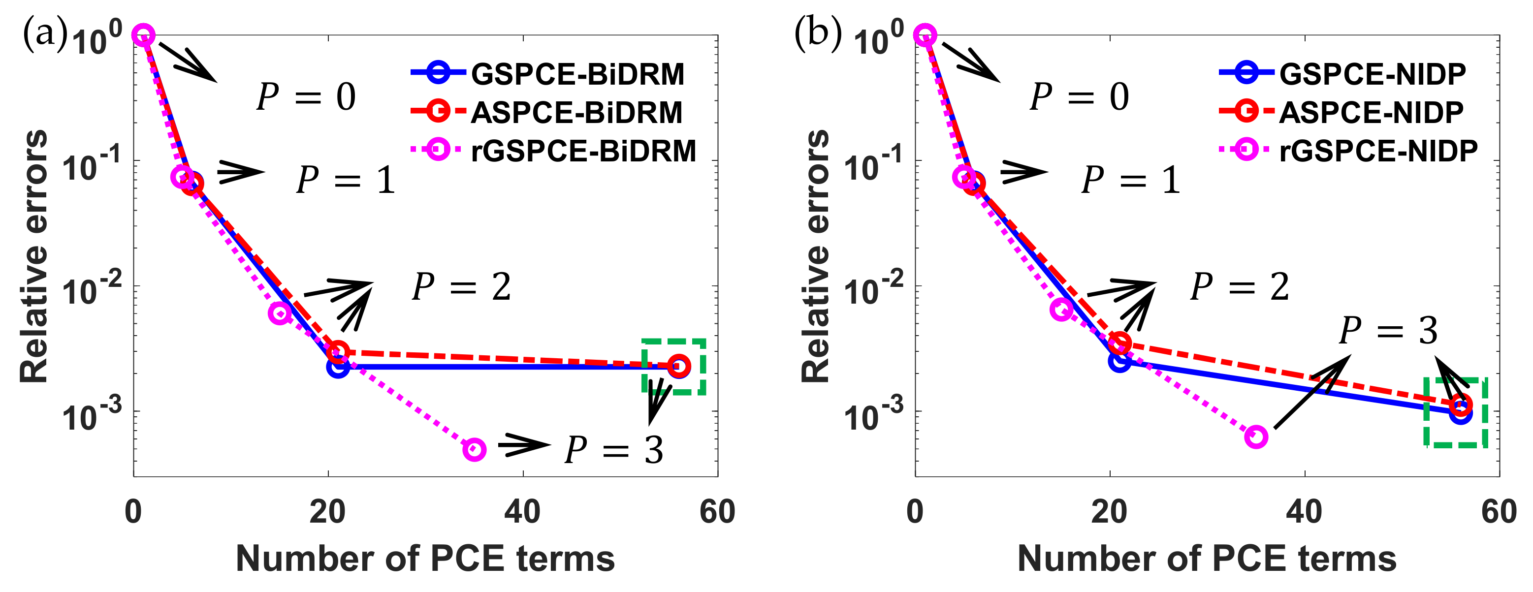
To compare the UQ accuracy with respect to different polynomial orders, the relative errors of the variance of were calculated at each simulation point in Figure 5. Note that the variance of can be analytically calculated with its PCE coefficients. Among these simulation points, 15 points were selected by dividing the total simulation range, i.e., from 0 to 120 in Figure 5, into 16 equal intervals. Following this, the average relative error of these 15 points was calculated for each case study and shown in Figure 6a. In addition, as in Example 1, the full tensor product grid-based NIDP was also conducted to demonstrate the performance of the proposed algorithm in terms of the UQ accuracy and computational efficiency. The simulation results with the NIDP-based approaches are given in Figure 6b.

Figure 6.
Comparison of the average relative error of the variance for with different (a) BiDRM- and (b) NIDP-based PCE approaches.
As can be seen in Figure 6a,b, the average relative errors decrease as the polynomial order increases in all case studies. It was also found that the convergence rate of the GSPCE-based algorithm is slightly faster than the ASPCE-based method. Notably, the rGSPCE-based method outperforms other case studies when was set to 3. In addition, it was found that the relative errors of the GSPCE- and ASPCE-BiDRM case studies in Figure 6a are slightly larger, compared to the GSPCE- and AGSPCE-NIDP in Figure 6b. This is because the BiDRM-based approach requires a smaller number of evaluations (), as compared to the NIDP-based approach (see Table 6). However, when was 3, we found that the relative error of the rGSPCE-BiDRM is lower than the rGSPCE-NIDP. This shows the advantage of combining the GS and gDRM with PCE, which reduces both the dimensionality of random space and the number of evaluations.

Table 6.
Summary of the number of PCE coefficients and the number of evaluations in Example 2.
We also studied the computational cost for each case study. Table 6 summarizes the number of PCE coefficients of model response and the number of evaluations required to calculate a coefficient with different algorithms. As seen in Table 6, for the GSPCE and ASPCE-based case studies, the number of PCE coefficients of is 6, 21, and 56, when was set to 1, 2, and 3, respectively. In contrast, the rGSPCE-based algorithm requires fewer PCE terms. Of note: the BiDRM approximates a five-dimensional integral in the spectral projection with 5 one- and 10 two-dimensional ones for the GSPCE- and ASPCE-based case studies. In contrast, a four-dimensional integral is converted into 4 one- and 6 two-dimensional ones in the rGSPCE-based case study. The lower-dimensional integrals were calculated with Gauss quadrature rules, and the number of quadrature points for each dimension was 5. Thus, the number of evaluations for the GSPCE- and ASPCE-BiDRM case studies is , according to the definition in (22). For the rGSPCE-BiDRM method, the number of evaluations is calculated as . For the NIDP-based case studies, the number of evaluations to solve a PCE coefficient is for both the GSPCE- and ASPCE-NIDP and in the rGSPCE-NIDP, when the full tensor product grid was used. As in the previous example, the computational time for four different case scenarios (i.e., three BiDRM-based methods and the ASPCE-NIDP method) is summarized in Table 7.

Table 7.
Summary of the computational time to quantify uncertainty in model output in Example 2.
As seen in Table 7, the computational time for the simulation in Figure 5 in each case study increases as increases. In addition, as compared to the ASPCE-based case studies, it was found the GSPCE-based case study requires more time to save and reload the numerical expressions of polynomial basis functions, since each parametric uncertainty has its own basis functions. However, it is important to note that the computational time for the rGSPCE-based case study is significantly smaller than the other three case studies, including the ASPCE-NIDP. This shows the superior performance of the rGSPCE-BiDRM based method, compared to the other methods (e.g., ASPCE-BiDRM and ASPCE-NIDP) in terms of computational efficiency.
3.3. Example 3: Continuously Stirred Tank Reactor (CSTR) with a Series Reaction
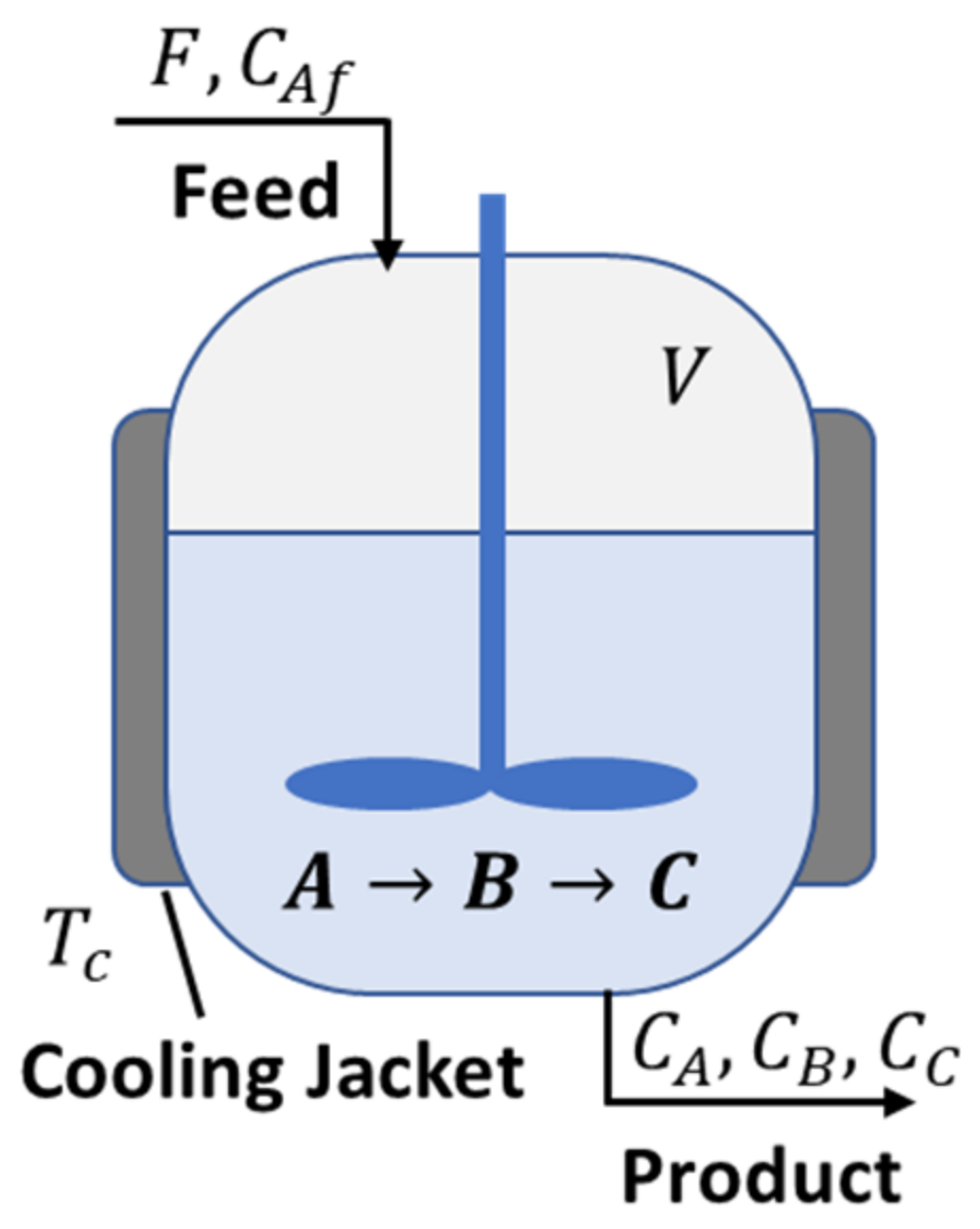
A continuously stirred tank reactor (CSTR) as in Figure 7 was chosen to show the efficiency of the UQ algorithm in this work, where irreversible reactions occur [43]. The pure material enters the reactor through the inlet stream and the concentrations of species and are initially set to zero. Since it is desired to reach the maximum conversion of , we focus on quantifying the effect of uncertainty on the concentration of .
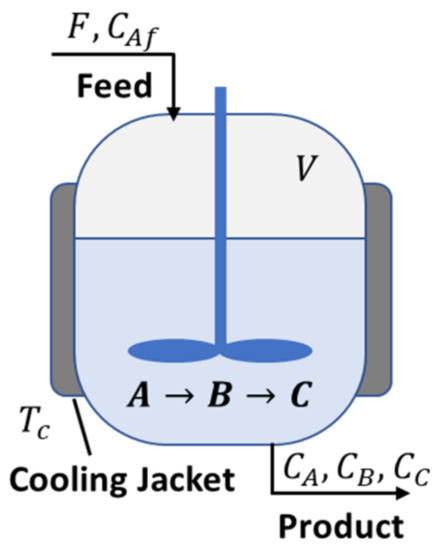
Figure 7.
Illustration of a continuously stirred tank reactor (CSTR) with a series reaction [43].
The models to describe the dynamics of the CSTR are given as [43]:
where , , and are the concentrations of , , and , respectively, and the temperature is the manipulated variable that is set to 400 K. Model parameters in (33)–(35) are listed in Table 8.

Table 8.
Description of model parameters in Example 3 [43].
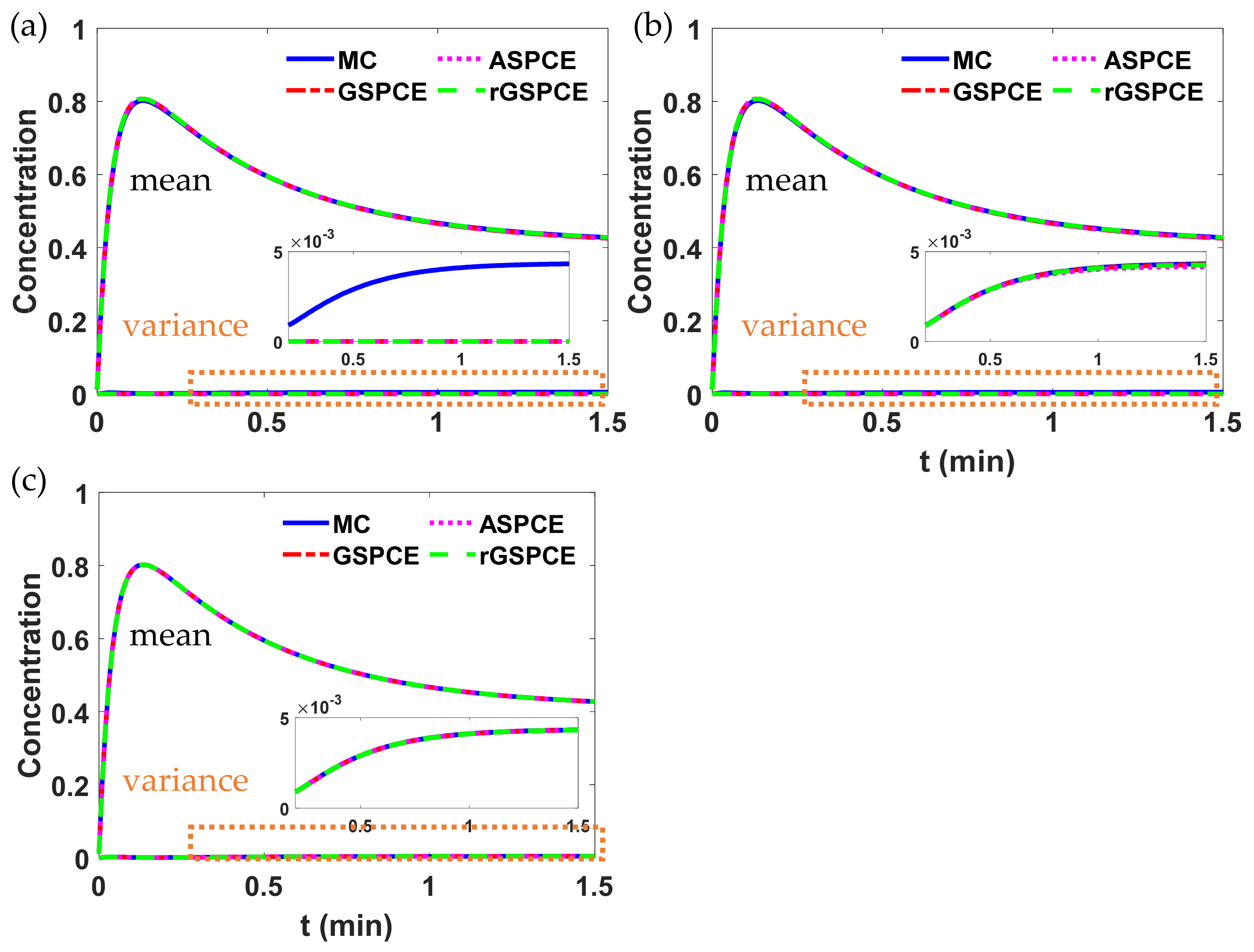
As in Table 8, three parameters, , , and , are assumed to follow a Weibull distribution. The rest of the parameters are described by standard distributions (e.g., uniform or normal). Since there are 7 parametric uncertainties, a seven-dimensional random space () is considered. In this example, a 1% variation around each mean value of the uncertain parameters and was introduced, and the rest of the parameters are assumed to have a 10% variation around each mean value. As in Examples 1 and 2, three case studies were conducted by combining the GSPCE, ASPCE, and rGSPCE with the BiDRM, respectively. For the GSPCE-based case study, PCE expressions of , , and were constructed using the modified GS, whereas the PCE expressions of , , and were approximated with the orthogonal polynomial basis functions in the Askey scheme for the ASPCE-based case study. For the rGSPCE-based case study, two uncertainties and (i.e., ) were treated as one uncertainty (i.e., the similarity parameter described in Section 2.3), which results in a six-dimensional random space (). As done in Examples 1 and 2, MC was implemented for comparison purposes, where 106 samples for each parametric uncertainty were used. Uncertainty in concentration was studied for each case study with respect to different polynomial orders of each uncertainty (i.e., was set to 0, 1, and ), and the simulation results are shown in Figure 8.
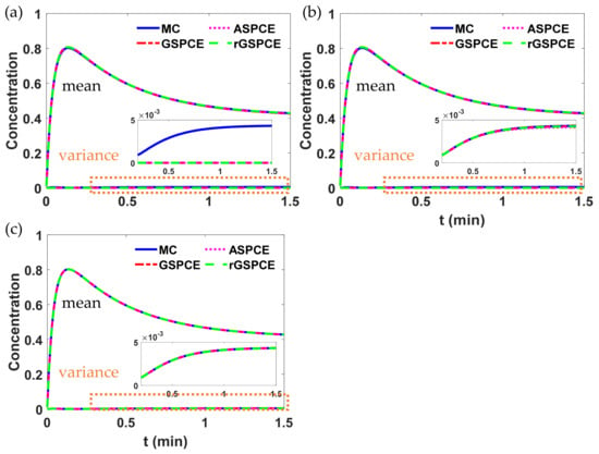
Figure 8.
Simulation results of concentration with different polynomial orders () in each case study: (a) , (b) , and (c) .
As seen in Figure 8, as the polynomial order of each uncertainty increases, the UQ accuracy of different methods can be improved. To quantify the UQ accuracy, the relative error of the variance of was calculated at each time instant in Figure 8. However, for clarity, the average of relative errors at 15 selected time instants are shown in Figure 9a for different case scenarios (i.e., GSPCE-, ASPCE-, and rGSPCE-BiDRM). As done in Examples 1 and 2, we also investigated the non-intrusive methods (NIDP) for comparison purposes. The results of NIDP-based approaches are shown in Figure 9b. The number of PCE terms and the number of evaluations for each polynomial order with respect to different approaches are summarized in Table 9.
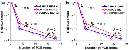
Figure 9.
Comparison of the average relative error of the variance for for with different (a) BiDRM- and (b) NIDP-based PCE approaches.

Table 9.
Summary of the number of PCE coefficients and the number of evaluations in Example 3.
The number of evaluations in Table 9 was determined by counting the total number of quadrature points to approximate each integral. For example, the number of evaluations to calculate each PCE coefficient is 561 for the GSPCE- and ASPCE-BiDRM, since there are 7 one- and 21 two-dimensional integrals resulting from the BiDRM, i.e., . In contrast, the number of evaluations to calculate a PCE coefficient is 406 for the rGSPCE-BiDRM since there are 6 one- and 15 two-dimensional integrals, i.e., . In addition, for the NIDP-based approaches, the number of evaluations to approximate each coefficient is calculated as in both the GSPCE- and ASPCE-NIDP and in the rGSPCE-NIDP. As compared to Example 2, a larger number of evaluations was used here for the NIDP-based approaches, since there are more uncertainties.
As seen in Figure 9, the average relative error decreases, as the polynomial order increases. In addition, the GSPCE- and rGSPCE-based algorithms exhibit smaller errors, as compared to the ASPCE-based algorithm. Note that the requisite number of PCE coefficients are the same in GSPCE- and ASPCE-based algorithms, while the rGSPCE-based algorithm needs a smaller number of PCE terms as in Table 9. In addition, the simulation results in Figure 9 shows that the BiDRM-based approaches provide as accurate results as the NIDP-based approaches, even with a smaller number of evaluations . Specifically, the rGSPCE-BiDRM has an average relative error of ~0.00154, and the error with the rGSPCE-NIDP is ~0.00153. As seen, the difference in the average relative error between the two approaches is insignificant. However, the algorithm in the work that combines GSPCE- (or rGSPCE-) and BiDRM can outperform the NIDP-based methods in terms of computational cost, since a smaller number of evaluations is required as in Table 9. We also studied the computational time to calculate PCE coefficients with respect to three BiDRM-based methods (i.e., GSPCE-, ASPCE-, and rGSPCE-BiDRM) and the ASPCE-NIDP in terms of CPU time, which is given in Table 10.

Table 10.
Summary of the computational time to quantify uncertainty in model output in Example 3.
As can be seen in Table 10, the rGSPCE-BiDRM requires the least computational time. For example, when was 2, the computational time of the rGSPCE-BiDRM was ~40% and ~30% lower than the GSPCE-BiDRM and ASPCE-BiDRM-based methods, respectively. In addition, it was found that the ASPCE-NIDP exhibits inferior computational time for each polynomial order to the rest of the case studies. This shows the performance of the proposed algorithm in this work in terms of computational efficiency, which combines the PCE with the modified GS algorithm and the BiDRM.
4. Conclusions
This paper presents an algorithm for efficient uncertainty quantification (UQ) under many parametric uncertainties that follow arbitrary distributions, which are not considered in the classic polynomial chaos expansion. The algorithm couples the modified Gram–Schmidt polynomial chaos expansion (GSPCE) with the generalized dimension reduction method (gDRM) to improve UQ accuracy and computational efficiency. The Gram–Schmidt orthogonalization can build appropriate orthogonal polynomial chaos basis functions for any type of arbitrary uncertainty. In addition, the algorithm can reduce the total number of required PCE terms to approximate the model output by combining several parametric uncertainties into a similarity parameter. To solve the PCE coefficients of model predictions quickly, the gDRM is used to approximate each high-dimensional integral from the inner product of the spectral projection with several lower-dimensional ones. To show the efficiency of the algorithm, engineering examples were used. The results show the approach in this work can significantly reduce the computational cost, while maintaining the UQ accuracy.
Author Contributions
Conceptualization, Y.D.; methodology, Y.D. and J.S.; validation, J.S.; investigation, J.S.; writing—original draft preparation, J.S.; writing—review and editing, Y.D.; supervision, Y.D. All authors have read and agreed to the published version of the manuscript.
Funding
This work was partially supported by the National Science Foundation, Division of Civil, Mechanical and Manufacturing Innovation (CMMI), under the award No. 1727487.
Institutional Review Board Statement
Not applicable.
Informed Consent Statement
Not applicable.
Data Availability Statement
Not applicable.
Conflicts of Interest
The authors declare no conflict of interest.
Appendix A
Gauss quadrature rule is a popular tool to calculate an integral with a weighted sum of its integrand evaluated at a set of node points [31,40]. In this work, the low-dimensional integrals from the gDRM as in (16) are numerically solved by the Gauss quadrature with five quadrature points and their corresponding weights. To construct a one-dimensional quadrature rule for an arbitrary random variable, let us consider a function over the support , , where is a single random variable (e.g., as described in Section 2.1). Then, the five-point Gauss quadrature can be formulated as:
where is a weighting function determined by the PDF of random variable . The key to accurately evaluate the integral on the left side in (A1) is to determine the optimal quadrature points and weights (i.e., and where ). In the Gaussian quadrature, the quadrature points are readily defined as the roots of the orthogonal polynomials which has the same support range as the random variable . As illustrated in Section 2.2, orthogonal polynomials for any arbitrary random variable can be readily constructed via the GS algorithm. As compared to the quadrature points, i.e., the abscissas , the corresponding weights have to be evaluated. One way to determine the weights is to use a set of linear equations as in [44]:
where is 5 5 matrix, which is defined as below.
where are polynomials that include exactly one polynomial of order from 0 to 4, respectively, such that . The vectors and are given as in:
Note that each element in is exactly the raw moment of , i.e., (see (11) in Section 2.2). In summary, using both the optimal orthogonal polynomials obtained from the GS algorithm and the raw moments of any given arbitrary random variable, the quadrature points and the corresponding weights of the Gauss quadrature rule can be readily constructed for the PCE-based UQ method in this work.
References
- Sullivan, T. Introduction to Uncertainty Quantification; Springer Science and Business Media LLC: Berlin/Heidelberg, Germany, 2015. [Google Scholar]
- Duong, P.L.T.; Minh, L.Q.; Pham, T.N.; Goncalves, J.; Kwok, E.; Lee, M. Uncertainty quantification and global sensitivity analysis of complex chemical processes with a large number of input parameters using compressive polynomial chaos. Chem. Eng. Res. Des. 2016, 115, 204–213. [Google Scholar] [CrossRef]
- Du, Y.; Budman, H.; Duever, T. Parameter Estimation for an Inverse Nonlinear Stochastic Problem: Reactivity Ratio Studies in Copolymerization. Macromol. Theory Simul. 2017, 26, 1600095. [Google Scholar] [CrossRef]
- Kim, K.; Kim, J.; Kim, C.; Lee, Y.; Lee, W.B. Robust Design of Multicomponent Working Fluid for Organic Rankine Cycle. Ind. Eng. Chem. Res. 2019, 58, 4154–4167. [Google Scholar] [CrossRef]
- Kumar, D.; Budman, H. Applications of Polynomial Chaos Expansions in optimization and control of bioreactors based on dynamic metabolic flux balance models. Chem. Eng. Sci. 2017, 167, 18–28. [Google Scholar] [CrossRef]
- Schenkendorf, R.; Xie, X.; Krewer, U. An efficient polynomial chaos expansion strategy for active fault identification of chemical processes. Comput. Chem. Eng. 2019, 122, 228–237. [Google Scholar] [CrossRef]
- Yang, H.-Q.; Chen, X.; Zhang, L.; Zhang, J.; Wei, X.; Tang, C. Conditions of Hydraulic Heterogeneity under Which Bayesian Estimation is More Reliable. Water 2020, 12, 160. [Google Scholar] [CrossRef] [Green Version]
- Rahn, S.; Gödel, M.; Fischer, R.; Köster, G. Dynamics of a Simulated Demonstration March: An Efficient Sensitivity Analysis. Sustainability 2021, 13, 3455. [Google Scholar] [CrossRef]
- Hariri-Ardebili, M.; Mahdavi, G.; Abdollahi, A.; Amini, A. An RF-PCE Hybrid Surrogate Model for Sensitivity Analysis of Dams. Water 2021, 13, 302. [Google Scholar] [CrossRef]
- Seitz, G.; Mohammadi, F.; Class, H. Thermochemical heat storage in a lab-scale indirectly operated CaO/Ca(OH)2 reactor—numerical modeling and model validation through inverse parameter estimation. Appl. Sci. 2021, 11, 682. [Google Scholar] [CrossRef]
- Fishman, G.S. Monte Carlo: Concepts, Algorithms, and Applications; Springer: New York, NY, USA, 1996. [Google Scholar]
- Ghanem, R.G.; Spanos, P.D. Stochastic Finite Elements: A Spectral Approach; Springer Science and Business Media LLC: New York, NY, USA, 1991. [Google Scholar]
- Wiener, N. The Homogeneous Chaos. Am. J. Math. 1938, 60, 897. [Google Scholar] [CrossRef]
- Xiu, D.; Karniadakis, G.E. The Wiener—Askey Polynomial Chaos for Stochastic Differential Equations. SIAM J. Sci. Comput. 2002, 24, 619–644. [Google Scholar] [CrossRef]
- Eldred, M.; Burkardt, J. Comparison of Non-Intrusive Polynomial Chaos and Stochastic Collocation Methods for Uncertainty Quantification. In Proceedings of the 47th AIAA Aerospace Sciences Meeting including The New Horizons Forum and Aerospace Exposition, Orlando, FL, USA, 5–8 January 2009. [Google Scholar]
- Enderle, B.; Rauch, B.; Grimm, F.; Eckel, G.; Aigner, M. Non-intrusive uncertainty quantification in the simulation of turbulent spray combustion using Polynomial Chaos Expansion: A case study. Combust. Flame 2020, 213, 26–38. [Google Scholar] [CrossRef]
- Kaintura, A.; Dhaene, T.; Spina, D. Review of Polynomial Chaos-Based Methods for Uncertainty Quantification in Modern Integrated Circuits. Electronics 2018, 7, 30. [Google Scholar] [CrossRef] [Green Version]
- Xiu, D.; Karniadakis, G.E. Modeling uncertainty in steady state diffusion problems via generalized polynomial chaos. Comput. Methods Appl. Mech. Eng. 2002, 191, 4927–4948. [Google Scholar] [CrossRef]
- Sharma, G.S.; Faverjon, B.; Dureisseix, D.; Skvortsov, A.; MacGillivray, I.; Audoly, C.; Kessissoglou, N. Acoustic Performance of a Periodically Voided Viscoelastic Medium with Uncertainty in Design Parameters. J. Vib. Acoust. 2020, 142, 061002. [Google Scholar] [CrossRef]
- Henneberg, J.; Nieto, J.G.; Sepahvand, K.; Gerlach, A.; Cebulla, H.; Marburg, S. Periodically arranged acoustic metamaterial in industrial applications: The need for uncertainty quantification. Appl. Acoust. 2020, 157, 107026. [Google Scholar] [CrossRef]
- Masquelet, M.; Yan, J.; Dord, A.; Laskowski, G.; Shunn, L.; Jofre, L.; Iaccarino, G. Uncertainty Quantification in Large Eddy Simulations of a Rich-Dome Aviation Gas Turbine. In Proceedings of the ASME Turbo Expo 2017: Turbomachinery Technical Conference and Exposition, Charlotte, NC, USA, 26–30 June 2017. [Google Scholar]
- Zoccarato, C.; Gazzola, L.; Ferronato, M.; Teatini, P. Generalized Polynomial Chaos Expansion for Fast and Accurate Uncertainty Quantification in Geomechanical Modelling. Algorithms 2020, 13, 156. [Google Scholar] [CrossRef]
- Le Maître, O.P.; Knio, O.M. Spectral Methods for Uncertainty Quantification: With Applications to Computational Fluid Dynamics; Springer Science & Business Media: Berlin/Heidelberg, Germany, 2010. [Google Scholar]
- Xiu, D. Numerical Methods for Stochastic Computations: A Spectral Method Approach; Princeton University Press: Princeton, NJ, USA, 2010. [Google Scholar]
- Xu, J.; Kong, F. A cubature collocation based sparse polynomial chaos expansion for efficient structural reliability analysis. Struct. Saf. 2018, 74, 24–31. [Google Scholar] [CrossRef]
- Smolyak, S.A. Quadrature and interpolation formulas for tensor products of certain classes of functions. Sov. Math. Dokl. 1963, 4, 240–243. [Google Scholar]
- Judd, K.L.; Maliar, L.; Maliar, S.; Valero, R. Smolyak method for solving dynamic economic models: Lagrange interpolation, anisotropic grid and adaptive domain. J. Econ. Dyn. Control. 2014, 44, 92–123. [Google Scholar] [CrossRef] [Green Version]
- Son, J.; Du, Y. Comparison of intrusive and nonintrusive polynomial chaos expansion-based approaches for high dimensional parametric uncertainty quantification and propagation. Comput. Chem. Eng. 2020, 134, 106685. [Google Scholar] [CrossRef]
- Son, J.; Du, D.; Du, Y. Modified Polynomial Chaos Expansion for Efficient Uncertainty Quantification in Biological Systems. Appl. Mech. 2020, 1, 11. [Google Scholar] [CrossRef]
- Xu, H.; Rahman, S. A generalized dimension-reduction method for multidimensional integration in stochastic mechanics. Int. J. Numer. Methods Eng. 2004, 61, 1992–2019. [Google Scholar] [CrossRef] [Green Version]
- Venkateshan, S.; Swaminathan, P. Computational Methods in Engineering; Academic Press: Cambridge, MA, USA, 2014. [Google Scholar]
- Björck, Å. Numerics of Gram-Schmidt orthogonalization. Linear Algebra Appl. 1994, 197–198, 297–316. [Google Scholar] [CrossRef] [Green Version]
- Witteveen, J.A.; Bijl, H. Modeling Arbitrary Uncertainties Using Gram-Schmidt Polynomial Chaos. In Proceedings of the 44th AIAA Aerospace Sciences Meeting and Exhibit, Reno, NV, USA, 9–12 January 2006. [Google Scholar]
- Wan, X.; Karniadakis, G.E. Multi-Element Generalized Polynomial Chaos for Arbitrary Probability Measures. SIAM J. Sci. Comput. 2006, 28, 901–928. [Google Scholar] [CrossRef]
- Oladyshkin, S.; Nowak, W. Data-driven uncertainty quantification using the arbitrary polynomial chaos expansion. Reliab. Eng. Syst. Saf. 2012, 106, 179–190. [Google Scholar] [CrossRef]
- Witteveen, J.; Sarkar, S.; Bijl, H. Modeling physical uncertainties in dynamic stall induced fluid—Structure interaction of turbine blades using arbitrary polynomial chaos. Comput. Struct. 2007, 85, 866–878. [Google Scholar] [CrossRef]
- Giraud, L.; Langou, J.; Rozloznik, M. The loss of orthogonality in the Gram-Schmidt orthogonalization process. Comput. Math. Appl. 2005, 50, 1069–1075. [Google Scholar] [CrossRef] [Green Version]
- Springer, M.D. The Algebra of Random Variables; John Wiley and Sons: Hoboken, NJ, USA, 1979. [Google Scholar]
- Spanos, A. Probability Theory and Statistical Inference; Cambridge University Press: Cambridge, UK, 2019. [Google Scholar]
- McClarren, R.G. Gauss Quadrature and Multi-dimensional Integrals. In Computational Nuclear Engineering and Radiological Science Using Python; Academic Press: Cambridge, MA, USA, 2018; pp. 287–299. [Google Scholar]
- Fogler, H.S. Essentials of Chemical Reaction Engineering; Pearson Education: Upper Saddle River, NJ, USA, 2011. [Google Scholar]
- Yeo, Y.K. Chemical Engineering Computation with MATLAB®; CRC Press: Boca Raton, FL, USA, 2017. [Google Scholar]
- Tenny, M.J.; Rawlings, J.B.; Wright, S.J. Closed-loop behavior of nonlinear model predictive control. AIChE J. 2004, 50, 2142–2154. [Google Scholar] [CrossRef]
- Yang, S.; Xiong, F.; Wang, F. Polynomial Chaos Expansion for Probabilistic Uncertainty Propagation. In Uncertainty Quantification and Model Calibration; InTechOpen: London, UK, 2017. [Google Scholar]
Publisher’s Note: MDPI stays neutral with regard to jurisdictional claims in published maps and institutional affiliations. |
© 2021 by the authors. Licensee MDPI, Basel, Switzerland. This article is an open access article distributed under the terms and conditions of the Creative Commons Attribution (CC BY) license (https://creativecommons.org/licenses/by/4.0/).


