Numerical and Experimental Study of Aerodynamic Performances of a Morphing Micro Air Vehicle


Abstract
:1. Introduction
2. Theoretical Background
- (1)
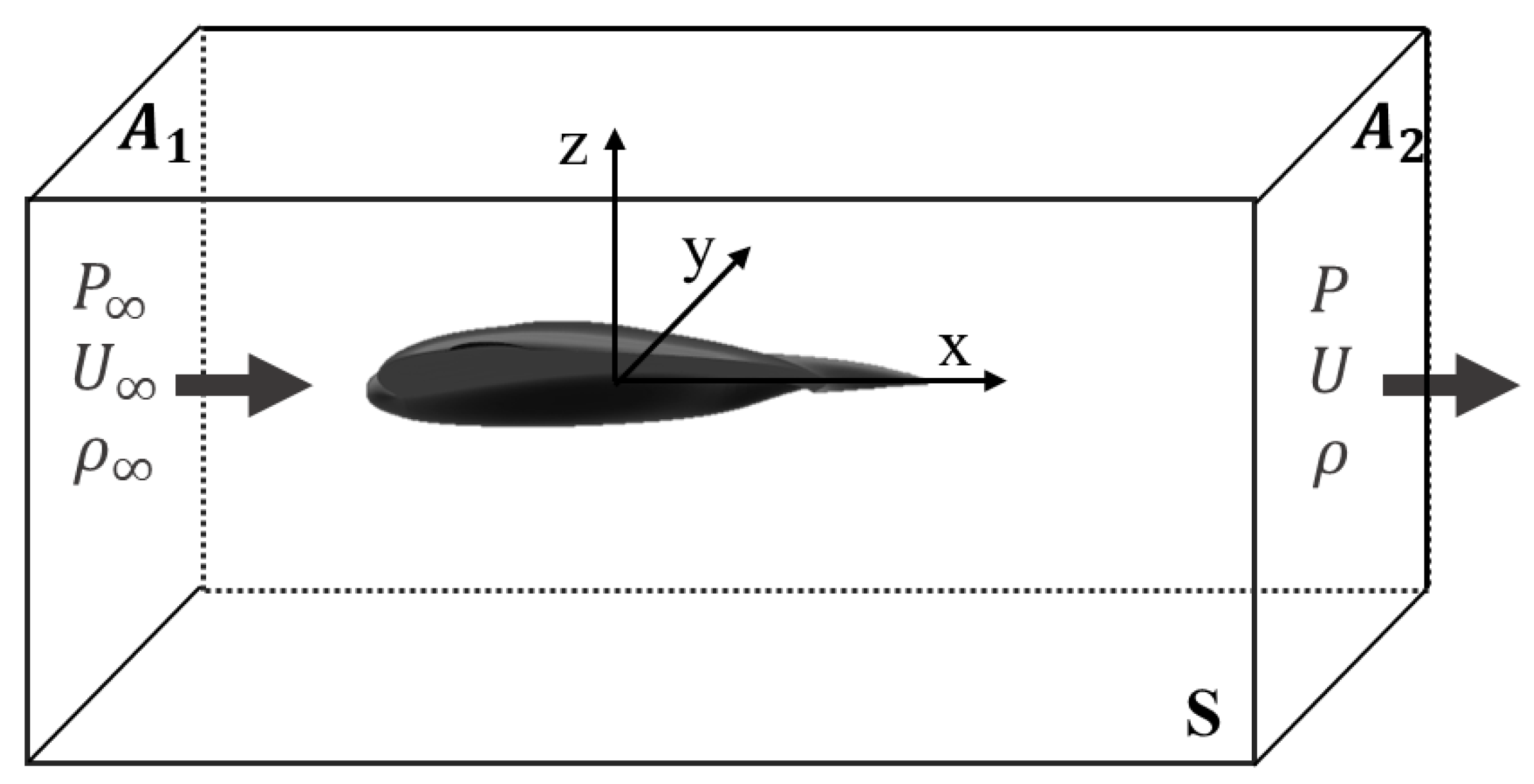
- The fluid flow measurements have to be performed in a transversal and downstream section to the MAV, plane A2 in Figure 1 (this plane is perpendicular to the X-axis, wind tunnel axis).
- (2)
- The flow in plane A2 is steady and incompressible.
- (3)
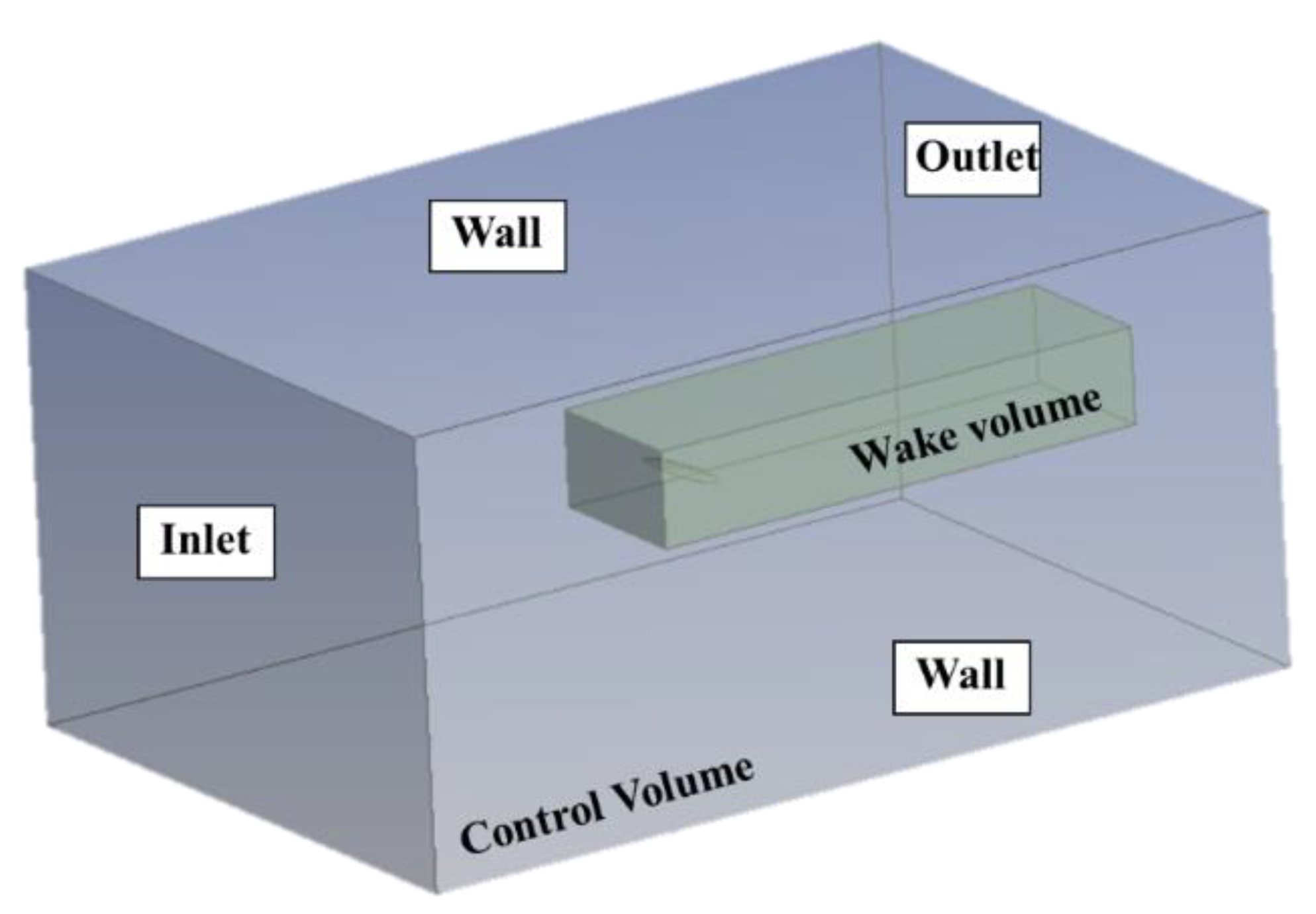
- The flow inside the fluid control volume without the MAV behaves as a uniform freestream parallel to the X-axis (wind tunnel axis) and its velocity is tangent to the walls (all surface of S (control volume) except to A1 and A2).
- (4)
- Fluid viscous stress terms are neglected in section A2 due to the distance of this plane is far away from the trailing edge of the MAV.
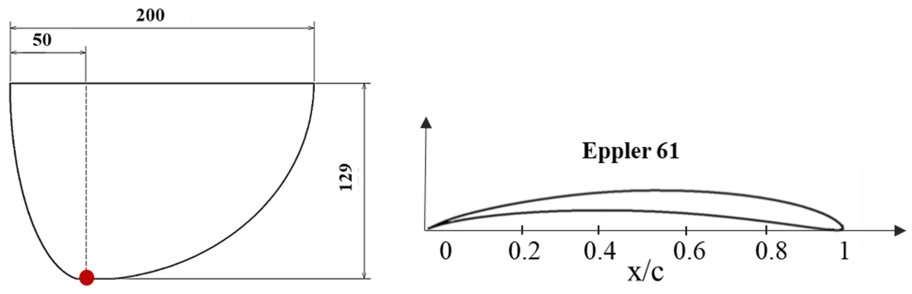
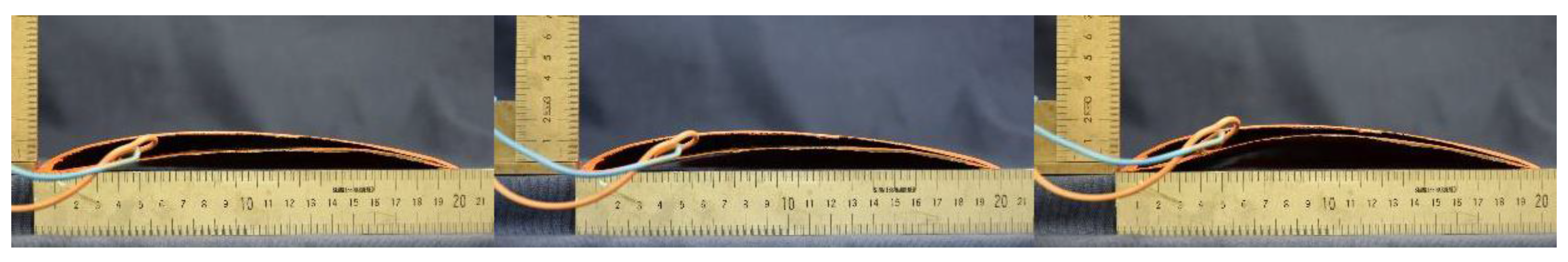
3. MAV with an Adaptative Wing Geometry
MAV Model
4. Computational Fluid Mechanics Investigation
4.1. Ansys-Fluent 2020
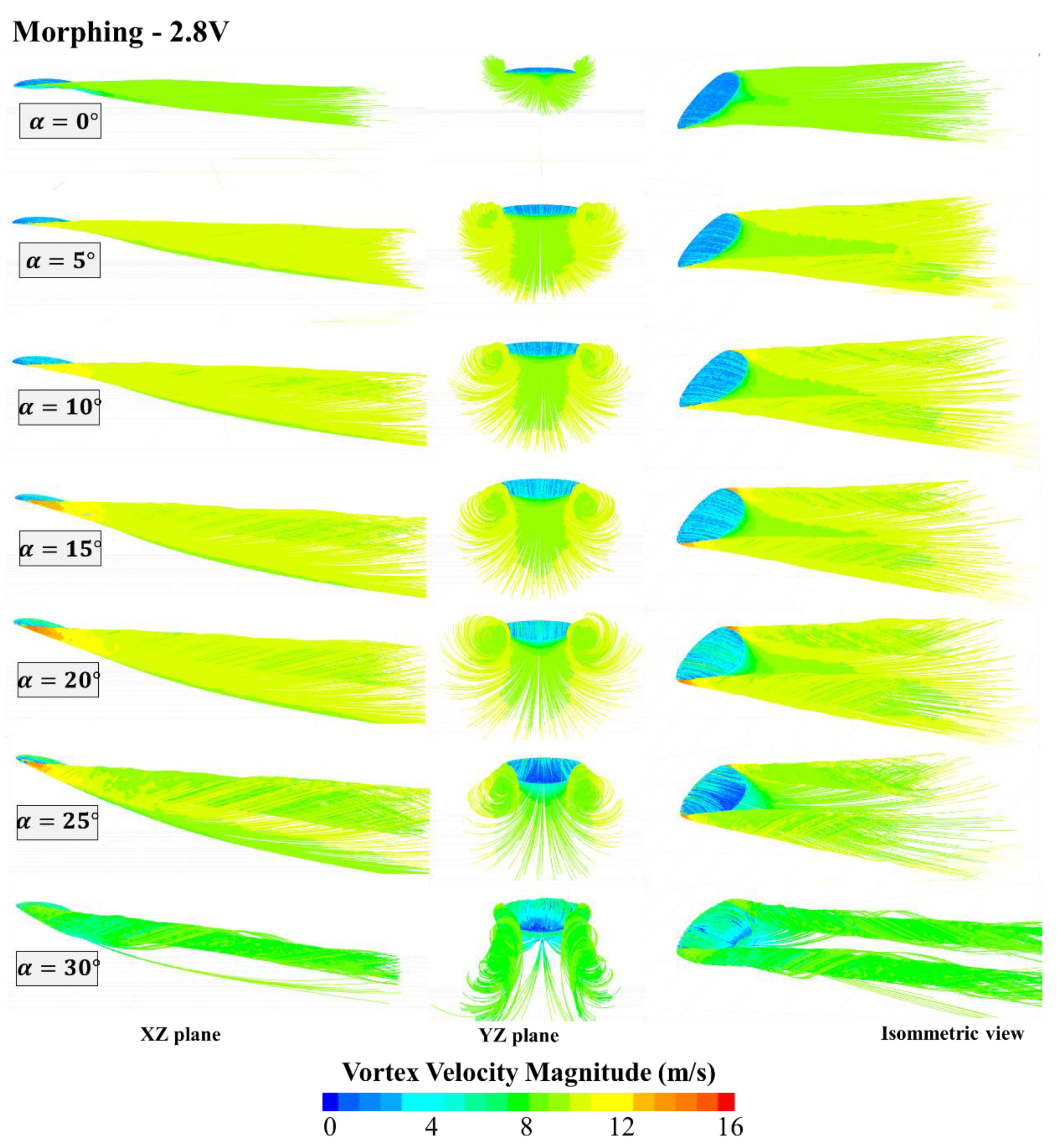
4.2. Computational Fluid Mechanics Results
4.2.1. Measurement Planes
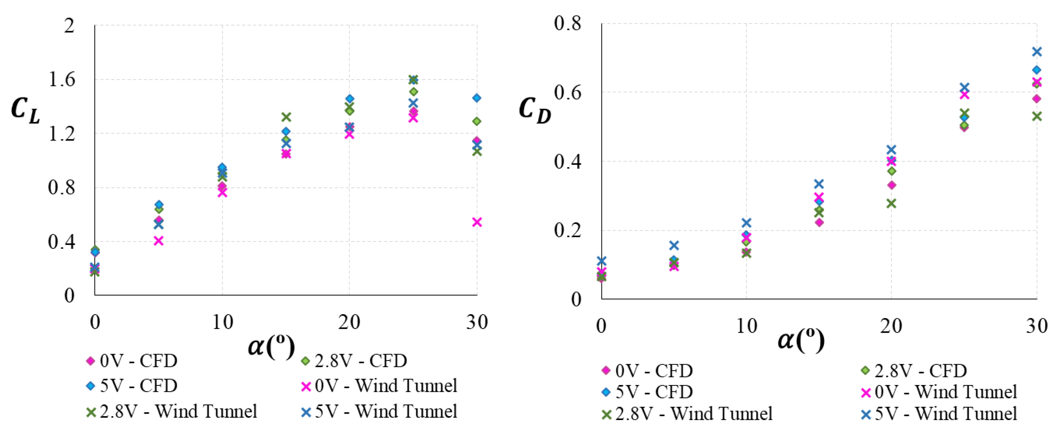
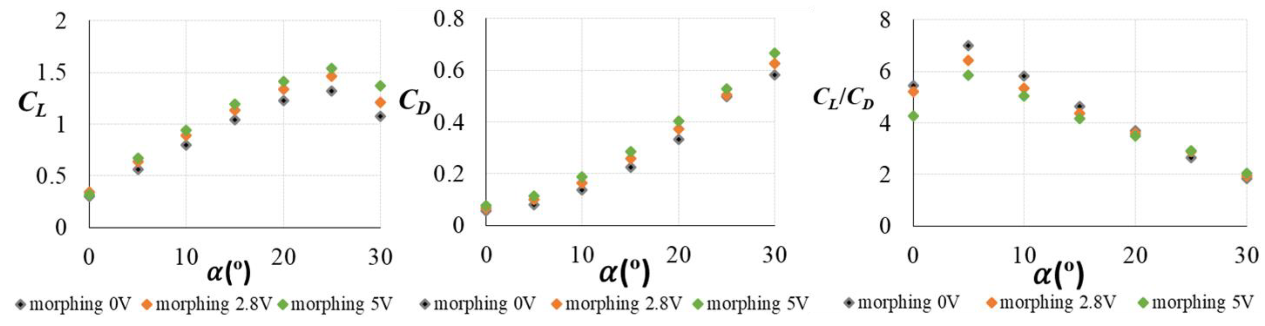
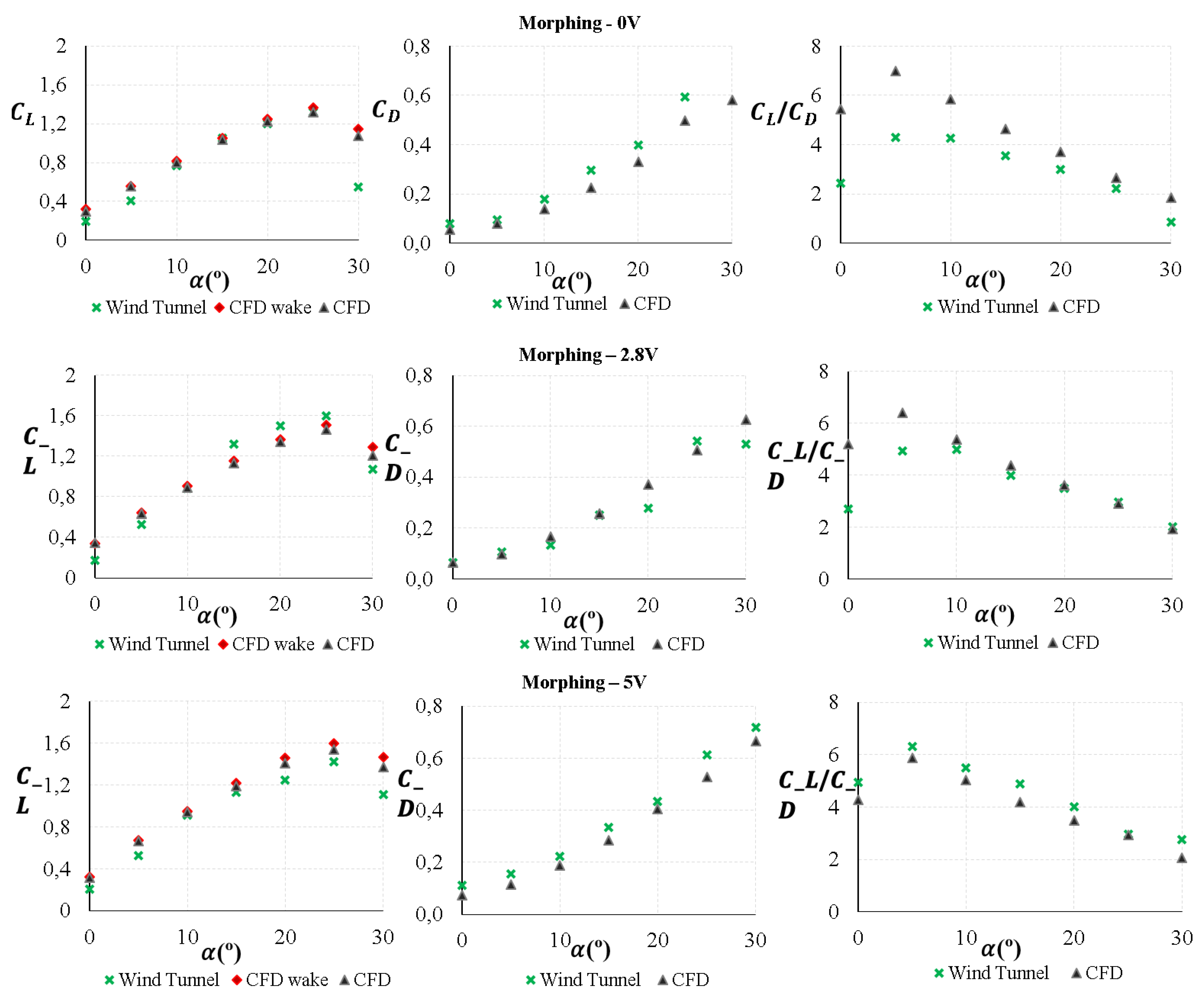
4.2.2. Lift and Total Aerodynamic Drag Coefficients and Lift/Drag Ratio
5. Experimental Study
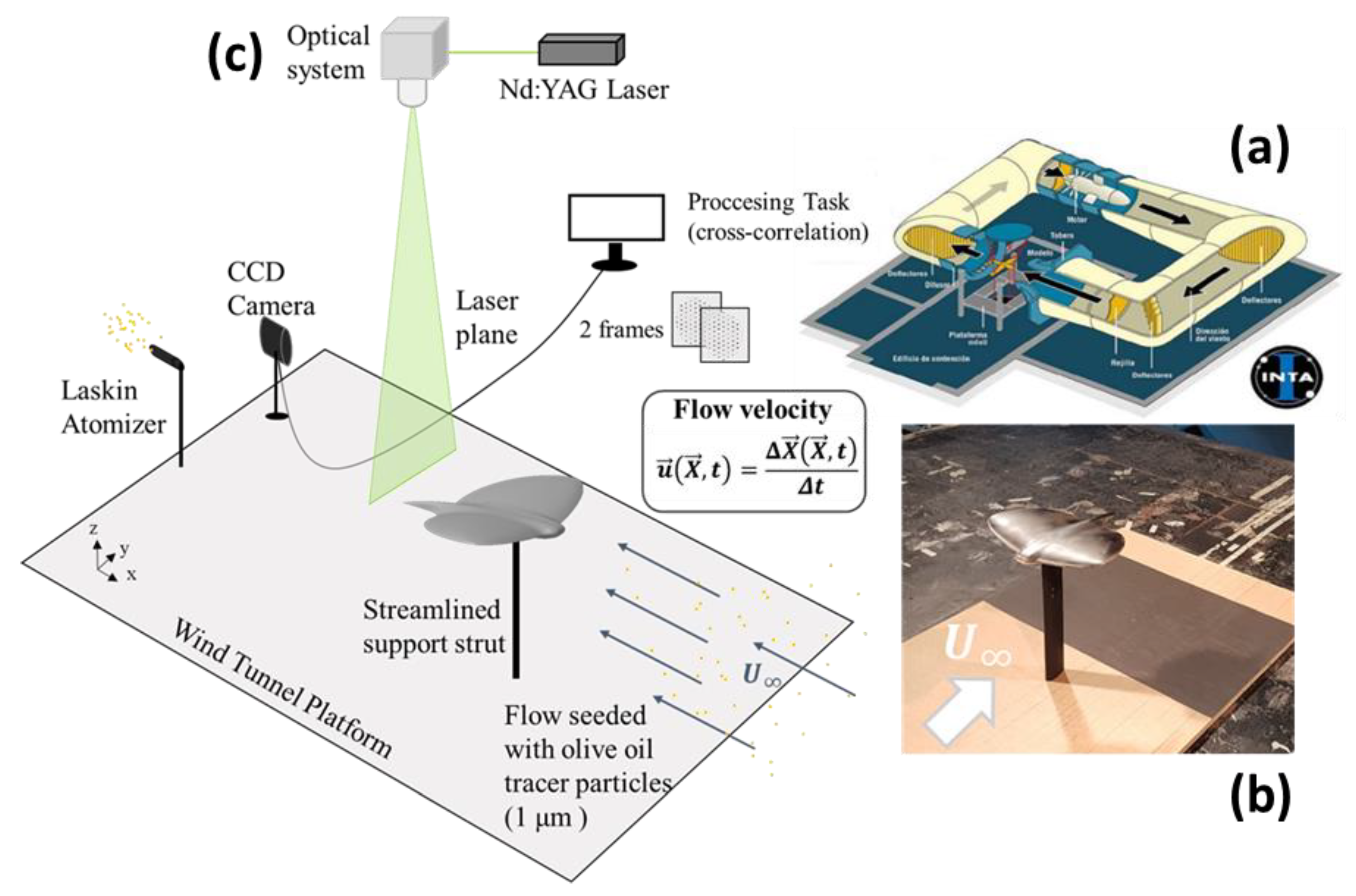
5.1. Wind Tunnel and Particle Image Velocimetry
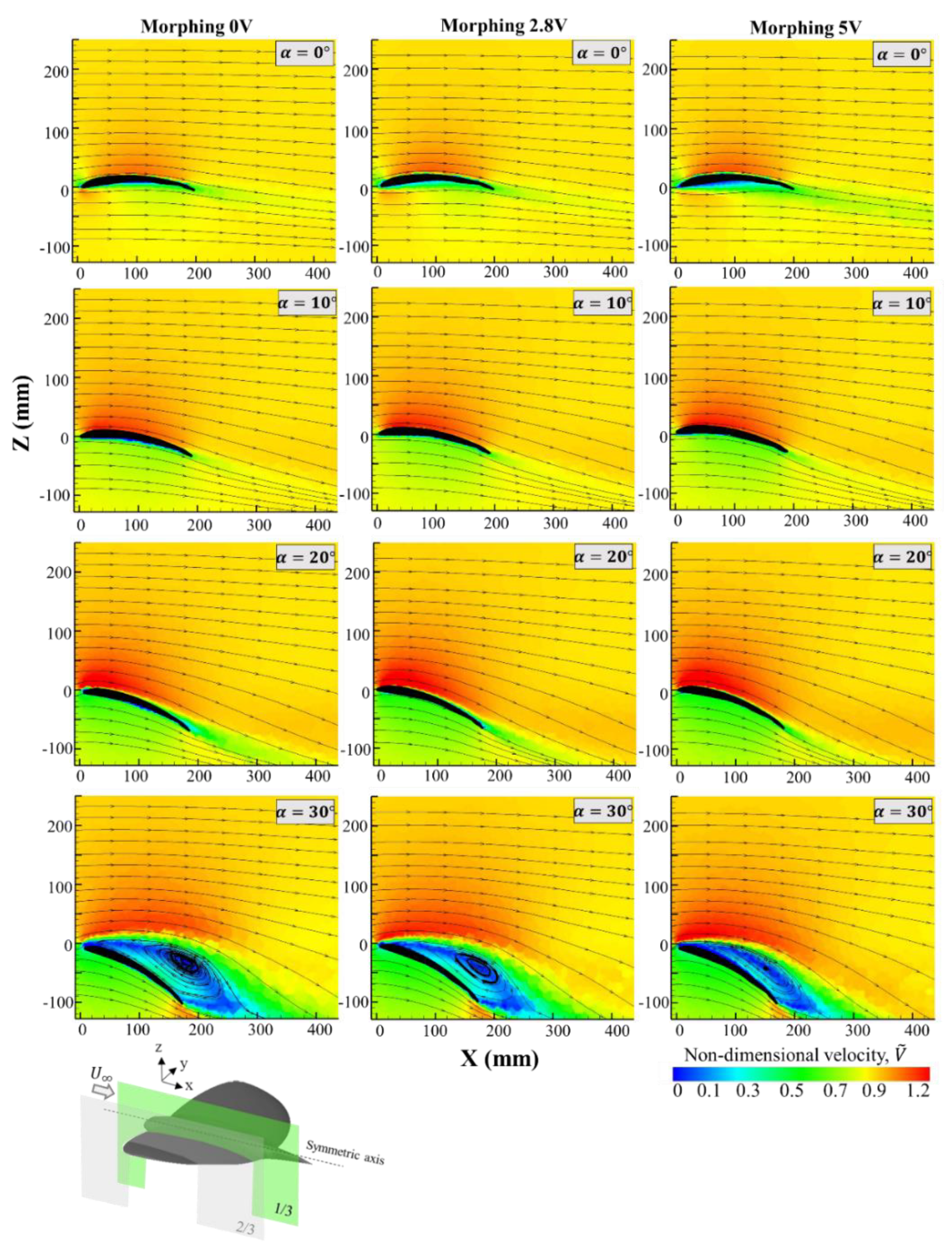
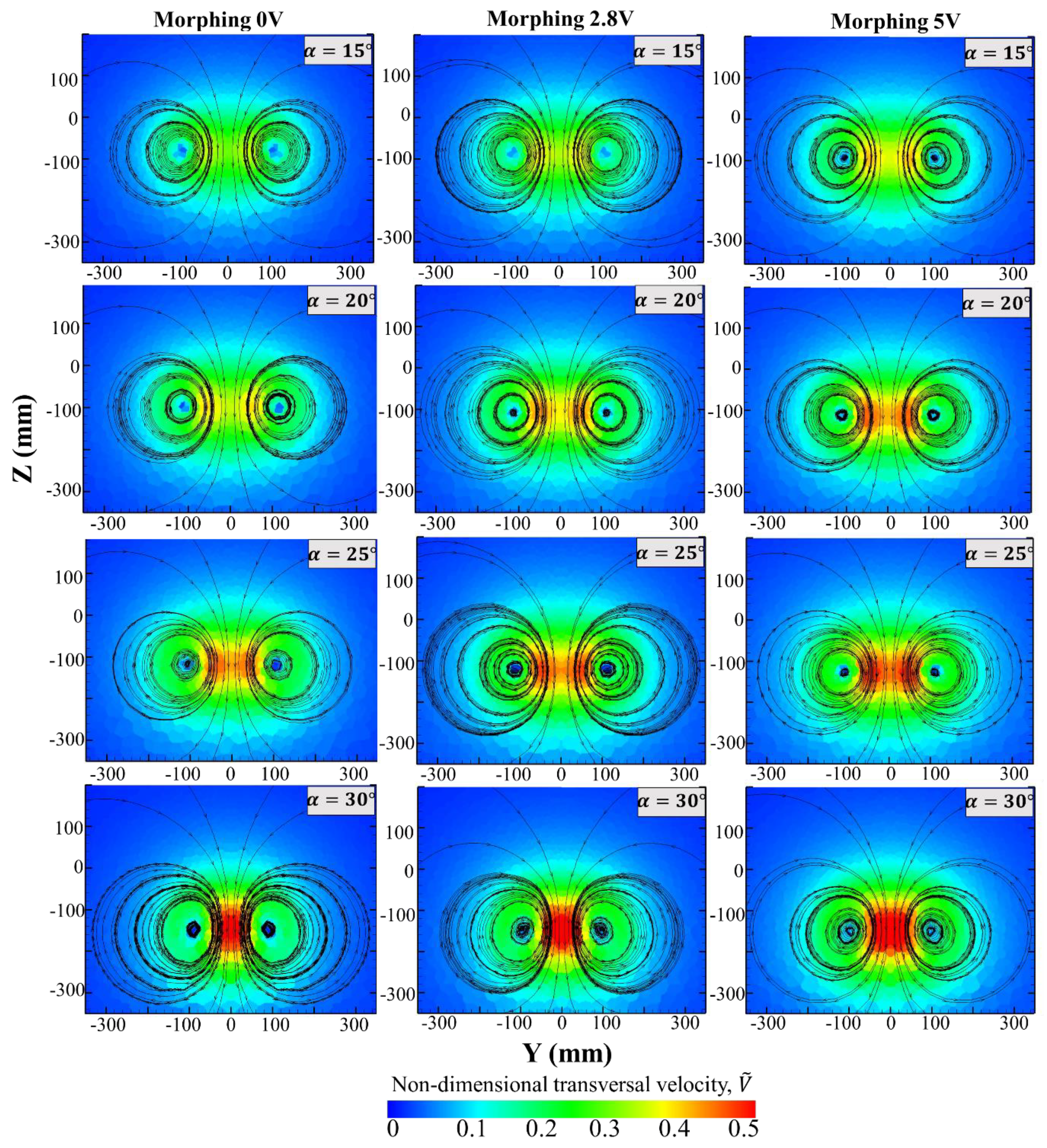
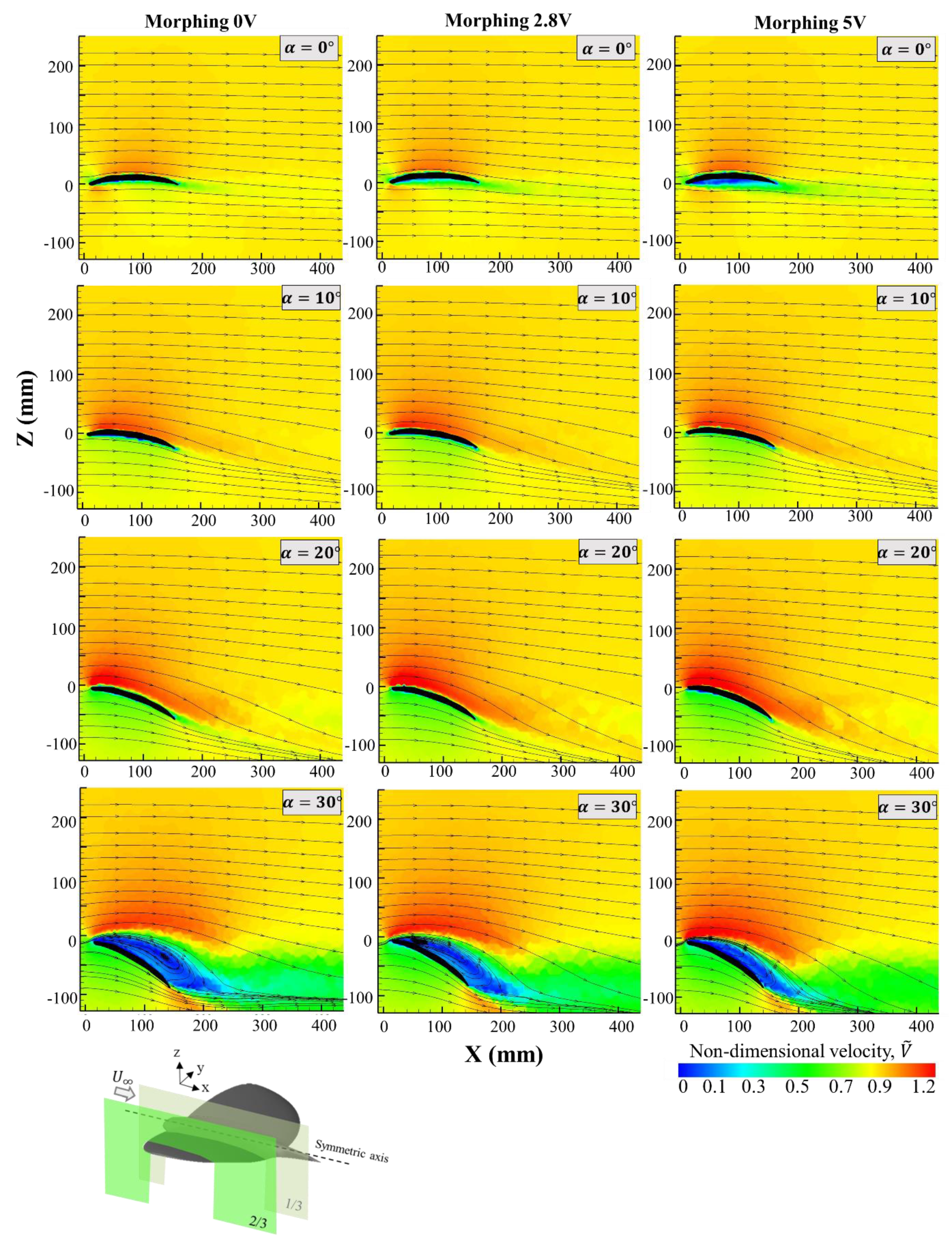
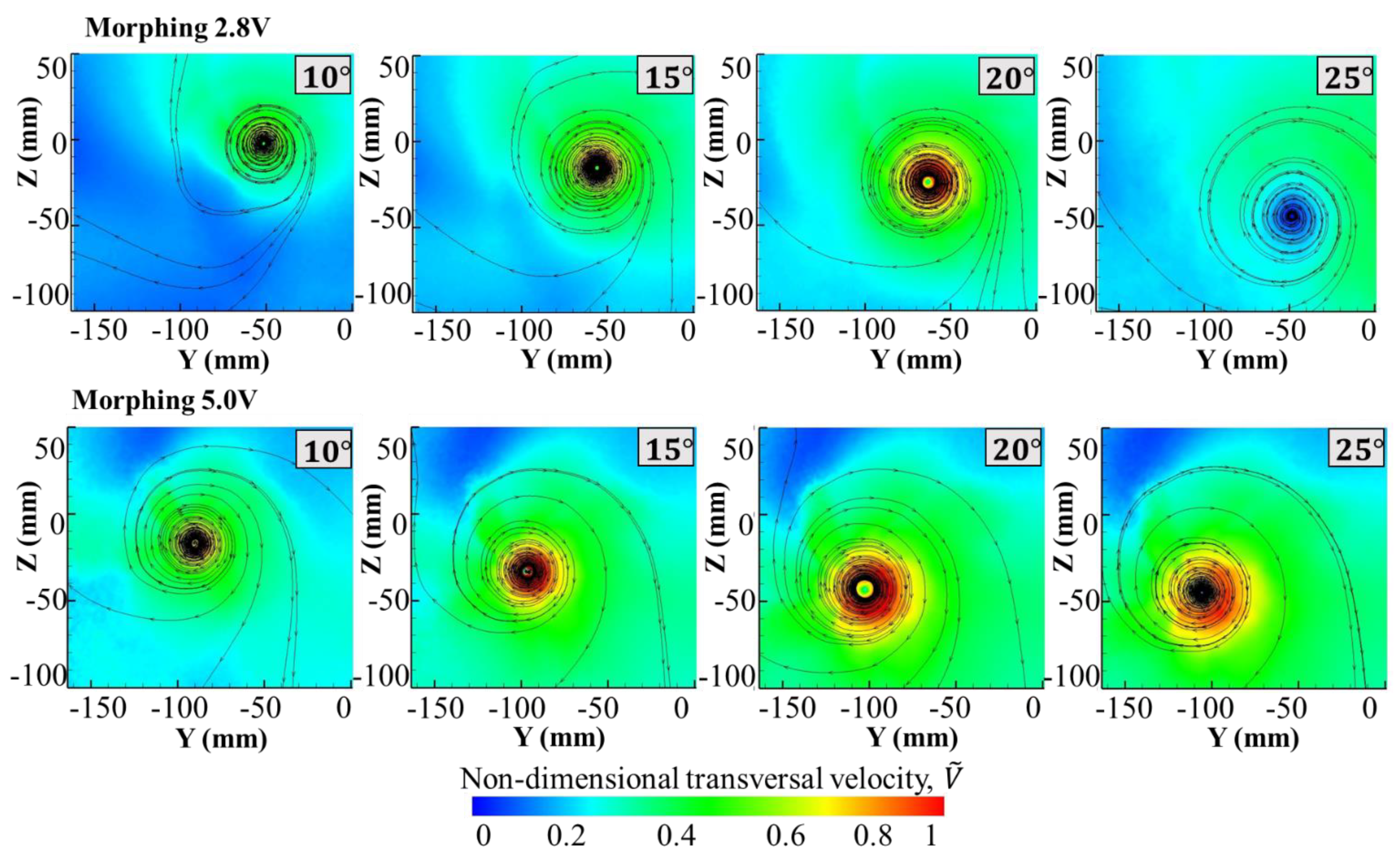
5.2. PIV Results
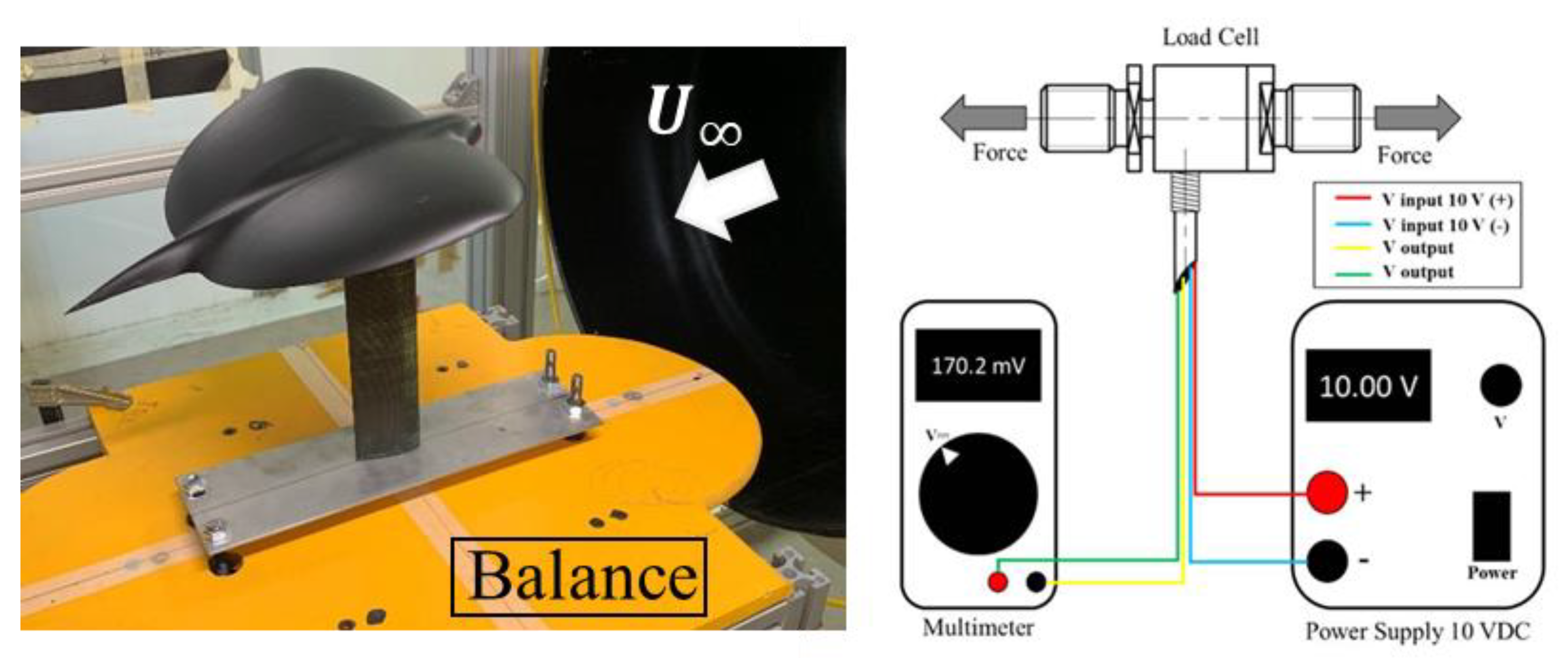
5.3. Balance Measurements
6. Comparative Analysis: CFD vs. Experimental
7. Conclusions
Author Contributions
Funding
Acknowledgments
Conflicts of Interest
References
- Moschetta, J.L. The aerodynamics of micro air vehicle: Technical challenges and scientific issues. Int. J. Eng. Syst. Model. Simul. 2014, 6, 134–148. [Google Scholar] [CrossRef]
- Hassanalian, M.; Abdelkefi, A. Design and manufacture of a fixed wing MAV with Zimmerman planform. In Proceedings of the AIAA SciTech, 54th AIAA Aerospace Sciences Meeting, Kissimmee, FL, USA, 4–8 January 2016. AIAA 2016-1743. [Google Scholar] [CrossRef]
- Marek, P.L. Design, Optimization and Flight Testing of a Micro Air Vehicle. Ph.D. Thesis, University of Glasgow, Glasgow, UK, 2008. [Google Scholar]
- Flake, J.; Frischknecht, B.; Hansen, S.; Knoebel, N.; Ostler, J.; Tuley, B. Development of the Stableyes Unmanned Air Vehicle. In Proceedings of the 8th International Micro Air Vehicle Competition, Tucson, AZ, USA, 10 April 2004; pp. 1–10. [Google Scholar]
- Stanford, B.; Sytsma, M.; Albertani, R.; Viieru, D.; Shyy, W.; Ifju, P. Static aeroelastic model validation of membrane micro air vehicle wings. AIAA J. 2007, 45, 2828–2837. [Google Scholar] [CrossRef]
- Min, Z.; Kien, V.K.; Richard, L.J.Y. Aircraft morphing wing concepts with radical geometry change. IES J. Part A Civ. Struct. Eng. 2010, 188–195. [Google Scholar] [CrossRef]
- Barbarino, S.; Bilgen, O.; Ajaj, R.M.; Friswell, M.I.; Inman, D.J. A review of morphing aircraft. J. Intell. Mater. Syst. Struct. 2011, 22, 823–877. [Google Scholar] [CrossRef]
- Sun, J.; Guan, Q. Morphing aircraft based on smart materials and structures: A state-of-the-art review. Intell. Mater. Syst. Struct. 2016, 27, 2289–2312. [Google Scholar] [CrossRef]
- Barcala-Montejano, M.A.; Rodríguez-Sevillano, A.; Crespo-Moreno, J.; Bardera Mora, R.; Silva-González, A.J. Optimized performance of a morphing micro air vehicle. In Proceedings of the Unmanned Aircraft Systems (ICUAS), 2015 International Conference, Denver, CO, USA, 12 June 2015. [Google Scholar] [CrossRef]
- Barcala-Montejano, M.A.; Rodríguez-Sevillano, A.; Bardera-Mora, R.; García-Ramirez, J.; Leon-Calero, M.; Nova-Trigueros, J. Development of a morphing wing in a micro air vehicle. In Proceedings of the 8th ECCOMAS Thematic Conference pon Smart Structures and Materials, SMART 2017, Madrid, Spain, 5–8 June 2017. [Google Scholar]
- Drela, M. Flight Vehicle Aerodynamics; The MIT Press: Cambridge, MA, USA, 2014; Chapter 5. [Google Scholar]
- Fan, Y.; Li, W. Review of far-field drag decomposition methods for aircraft design. J. Aircr. 2019, 56. [Google Scholar] [CrossRef]
- Betz, A. A method for the direct determination of profile drag. Z. Für Flugtech. Und Mot. 1925, 16, 42–44. [Google Scholar]
- Maskell, E.C. Progress towards a Method for the Measurement of the Components of the Drag of a Wing of Finite Span; RAE Technical Report 72232; Royal Aircraft Establishment RAE: Farnborough, Hampshire, 1972. [Google Scholar]
- Brune, G.W. Quantitative Three-Dimensional Low-Speed Wake Surveys; Boeing Commercial Airplane Group Seattle: Washington, DC, USA, 1991. [Google Scholar]
- Kusunose, K. Development of a universal wake survey data analysis code. In Proceedings of the 15th Applied Aerodynamics Conference, Atlanta, GA, USA, 23–25 June 1997. AIAA Paper 1997-2294. [Google Scholar] [CrossRef]
- Cummings, R.M.; Giles, M.B.; Shrinivas, G.N. Analysis of the elements of drag in three-dimensional viscous and inviscid flows. In Proceedings of the 14th Applied Aerodynamics Conference, New Orleans, LA, USA, 17–20 June 1996. AIAA Paper 1996-2482-CP. [Google Scholar] [CrossRef] [Green Version]
- Sor, S.; Bardera, R.; García-Magariño, A.; Matías García, J.; Donoso, E. Development and characterization of a low-cost wind tunnel balance for aerodynamic drag measurements. Eur. J. Phys. 2019, 40, 045002. [Google Scholar] [CrossRef]


| Parameter | Value |
|---|---|
| Wing tip chord | 0.025 m |
| Wing root chord | 0.200 m |
| Taper ratio | 0.124 |
| Aspect ratio | 2.500 |
| Wingspan | 0.320 m |
| Mean aerodynamic chord | 0.141 m |
| Mean geometry chord | 0.127 m |
| Wing reference area | 0.040 m2 |
| Dihedral length | 10° |
| Fuselage length | 0.3 m |
| Fuselage width | 0.06 m |
| Parameter | Value |
|---|---|
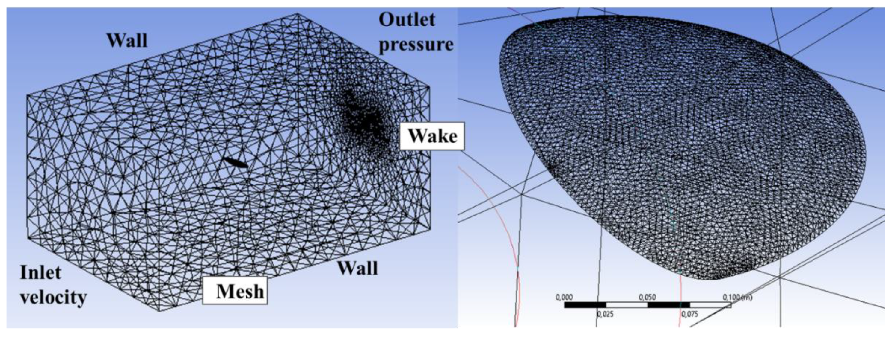
| Mesh type | Unstructured mesh |
| Smoothing | Medium |
| Inflation | Smooth |
| Relevant center | Fine |
| Span angle center | Fine |
| Maximum layers | 5 |
| Transition ratio | 0.3 |
| Minimum size | 5.7 mm |
| Maximum size | 116 mm |
| Growth rate | 1.2 |
| Nodes | 85,437 |
| Elements | 487,099 |
| Parameter | Value |
|---|---|
| At (time interval between laser pulses) | 22 μs |
| Camera CCD | Nikon NIKKOR 50 mm 1:1.4D |
| w (interrogation window size) | 32 × 32 pixels |
| Processing | 50% overlapping (Nyquist criteria). The correlation peak is adjusted to the subpixel accuracy Gaussian curve. |
| Post-processing algorithm | Local mean filter with a size of 3 × 3 pixels |
Publisher’s Note: MDPI stays neutral with regard to jurisdictional claims in published maps and institutional affiliations. |
© 2021 by the authors. Licensee MDPI, Basel, Switzerland. This article is an open access article distributed under the terms and conditions of the Creative Commons Attribution (CC BY) license (https://creativecommons.org/licenses/by/4.0/).
Share and Cite
Bardera, R.; Rodríguez-Sevillano, Á.A.; Barroso, E. Numerical and Experimental Study of Aerodynamic Performances of a Morphing Micro Air Vehicle. Appl. Mech. 2021, 2, 442-459. https://doi.org/10.3390/applmech2030025
Bardera R, Rodríguez-Sevillano ÁA, Barroso E. Numerical and Experimental Study of Aerodynamic Performances of a Morphing Micro Air Vehicle. Applied Mechanics. 2021; 2(3):442-459. https://doi.org/10.3390/applmech2030025
Chicago/Turabian StyleBardera, Rafael, Ángel A. Rodríguez-Sevillano, and Estela Barroso. 2021. "Numerical and Experimental Study of Aerodynamic Performances of a Morphing Micro Air Vehicle" Applied Mechanics 2, no. 3: 442-459. https://doi.org/10.3390/applmech2030025
APA StyleBardera, R., Rodríguez-Sevillano, Á. A., & Barroso, E. (2021). Numerical and Experimental Study of Aerodynamic Performances of a Morphing Micro Air Vehicle. Applied Mechanics, 2(3), 442-459. https://doi.org/10.3390/applmech2030025