Energy Minimization Scheme for Split Potential Systems Using Exponential Variational Integrators

Abstract

In previous works we developed a methodology of deriving variational integrators to provide numerical solutions of systems having oscillatory behavior. These schemes use exponential functions to approximate the intermediate configurations and velocities, which are then placed into the discrete Lagrangian function characterizing the physical system. We afterwards proved that, higher order schemes can be obtained through the corresponding discrete Euler–Lagrange equations and the definition of a weighted sum of “continuous intermediate Lagrangians” each of them evaluated at an intermediate time node. In the present article, we extend these methods so as to include Lagrangians of split potential systems, namely, to address cases when the potential function can be decomposed into several components. Rather than using many intermediate points for the complete Lagrangian, in this work we introduce different numbers of intermediate points, resulting within the context of various reliable quadrature rules, for the various potentials. Finally, we assess the accuracy, convergence and computational time of the proposed technique by testing and comparing them with well known standards.

1. Introduction

During the last few decades, there has been a growing interest in the development of numerical integration schemes for physical systems based on the theory of variations. Towards this aim, many authors suggested numerical methods that can be deduced through the discretization of the Hamilton’s principle, leading to the class of integration methods known as discrete variational integrators. Due to their derivation process, they show specific geometric advantages, especially when they are applied to solving mechanical systems. It is worth noting that the preservation of the geometric features of the dynamical system makes these methods appropriate for both conservative and nearly dissipative systems [1,2,3,4].

When solving numerically ordinary differential equations (ODEs), one of the most difficult problems is the derivation of solutions appropriate for systems presenting highly oscillatory behavior [1]. For such systems, it has been shown that standard numerical methods require a huge number of (time) steps to track the oscillations, while geometric integrators proved to be quite advantageous tools [5]. The latter class of integrators endow highly qualified simulations for long term integration processes without showing spurious effects (i.e., bad energy behavior appeared in traditional schemes for conservative systems) [5,6,7,8,9,10].

On the other hand, in solving numerically Hamiltonian systems, an interesting still open issue is related with the property of the corresponding potential-energy function to be analyzed in several components each of them representing strongly varying dynamics. These interactions often (mainly) lead to extremely stiff potentials that force the solution to oscillate with a very small time scale [5]. To derive numerical integration schemes that respect the geometric characteristics of such systems, following our previous work [11], we split their potential energy into one fast and one slow component. For the resulting energy functional, we subsequently derive a special kind of high order geometric schemes based on exponential variational integrators. The latter schemes may employ different quadrature rules in the different potentials involved in the corresponding discrete action. For the sake of completeness of the proposed schemes, we assess their accuracy, convergence and computational time while comparing them with some standard ones.

The remainder of the article is organized as follows. We start by recalling the Hamiltonian formalism via the definition of the exponential integrators (Section 2). Then, we briefly summarize the physical concepts of the Lagrangian mechanics that help us to introduce the new exponential variational integrators (Section 3). These integrators are afterwards extended appropriately in order to be applicable to Hamiltonian systems of which the potential term of the energy functional can be split in fast and slow parts (Section 4). In Section 5, we present the tests and discuss the level of accuracy, convergence and computational time of the new schemes coming out of several numerical experiments performed on the general N-body problem. Finally (Section 6), we summarize the main conclusions extracted in the present work.

2. Exponential Integrators

In previous works we developed exponential integrators for Hamiltonian systems satisfying differential equations of the form [5]

$$\ddot{q}+\mathsf{\Omega }q=g\left(q\right),g\left(q\right)=-\nabla U\left(q\right),$$

(1)

where $\mathsf{\Omega }$ denotes a diagonal matrix and $U\left(q\right)$ is a smooth potential function. Due to the nature of the problems, the entries $\omega$ of $\mathsf{\Omega }$ are assumed to have large modulus. In this work, we focus on the long time behavior of the numerical solutions, emphasizing on the special cases when $\omega h$ (with h being the time step) is relatively large [10].

Following Ref. [5], an exact discretisation of $q\left(t\right)$ in (1) can be written as

$$q_{n+1}-2cos\left(\omega h\right)q_n+q_{n-1}=0,n\in \mathbb{Z}$$

(2)

Using the above anzatz, we can consider general numerical schemes defined as

$$q_{n+1}-2cos\left(\omega h\right)q_n+q_{n-1}=h^2\psi \left(\omega h\right)g\left(\varphi \left(\omega h\right)q_n\right).$$

(3)

The latter expressions are fully determined via the functions $\psi \left(\omega h\right)$ and $\varphi \left(\omega h\right)$ which are assumed to be even and real-valued functions satisfying the condition $\psi \left(0\right)=\varphi \left(0\right)=1$, see [5]. We note that, due to the presence of exponential terms in the above expressions, the resulting numerical schemes are known as exponential integrators (see, e.g., Appendix of Ref. [12]).

3. Variational Integrators Based on Interpolation Techniques

For the derivation of high order variational integrators we are interested in this work, we need to recall basic concepts from the discrete variational calculus [4,8,10]. Then, we define a discrete Lagrangian $L_d$ as a function of positions only, i.e.,

$$L_d:Q\times Q\to \mathbb{R}.$$

(4)

(Q represents a given configuration space). The discrete Lagrangian $L_d$, is normally obtained from a continuous Lagrangian $L(q,\dot{q})$ defined via the known map

$$L:TQ\to \mathbb{R}$$

(5)

(T represents the tangent space of the configuration space Q). Towards this aim, an approximation must be considered of the form [4,10]

$$L_d(q_k,q_{k+1})\approx {\int }_{t_k}^{t_{k+1}}L(q,\dot{q})dt.$$

(6)

($t_k$ and $t_{k+1}$ denote adjacent time moments of the time discretization grid, with $t_{k+1}-t_k=h$). In a similar way, the action sum $S_d$ is defined via the map

$$S_d:Q^{N+1}\to \mathbb{R},N\in \mathbb{N}.$$

(7)

Obviously, the action sum $S_d$ must correspond to a set of discrete Lagrangians $L_d$, connected through the use of a discrete trajectory ${\gamma }_d=(q_0,\dots ,q_N)$ as [10]

$$S_d\left({\gamma }_d\right)=\sum _{k=1}^{N-1}{L}_d(q_{k-1},q_k).$$

(8)

Subsequently, if we denote the dual space of $TQ$ by $T^{*}Q$, the latter space consists of covectors $\alpha$ such that

$$\alpha \in T_{(x_1,x_2)}^{*}(Q\times Q).$$

(9)

In general, any covector $\alpha$ can be decomposed as

$$\alpha ={\alpha }_1+{\alpha }_2,\mathrm{where}{\alpha }_i\in T_{x_i}^{*}(Q\times Q),\mathrm{with}i=1,2.$$

(10)

A special case of this type of covectors are the $d{L}_d(q_0,q_1)$ which, by applying the above definition, can be decomposed similarly as [4,10]

$$d{L}_d(q_0,q_1)=D_1{L}_d(q_0,q_1)+D_2{L}_d(q_0,q_1),$$

(11)

where $D_i{L}_d$ indicates the derivative with respect to the i-th argument of $L_d$.

Furthermore, according to the discrete variational principle, the solutions of the discrete system of equations determined by the Lagrangian $L_d$ must extremize the action sum $S_d$ of Equation (8) for given fixed points $q_0$ and $q_N$. Extremizing $S_d$ over all the intermediate points of the discrete trajectory ${\gamma }_d$, we obtain the system of difference equations

$$D_2{L}_d(q_{k-1},q_k)+D_1{L}_d(q_k,q_{k+1})=0,k=1,\dots ,N-1,$$

(12)

The latter equations, are usually called discrete Euler–Lagrange equations [4,10].

Guided by the definition of the conjugate momenta in the case of the continuous mechanics, at this point we consider the discrete conjugate momenta at the time steps k and $k+1$ as

$$\begin{array}{ccc}\hfill p_k& =& -D_1{L}_d(q_k,q_{k+1}),\hfill \\ \hfill p_{k+1}& =& D_2{L}_d(q_k,q_{k+1}),k=0,\cdots ,N-1,\hfill \end{array}$$

(13)

which are known as “position-momentum forms” of variational integrators. The latter are used to obtain, at the first step, the $(q_1,p_1)$ when the initial condition $(q_0,p_0)$ are provided [4].

3.1. High Order Variational Integrators

In order to derive (more accurate) high order methods, we approximate the action integral along the curve segment bounded by the two endpoints $q_k$ and $q_{k+1}$ by utilizing a discrete Lagrangian that depends only on the given end points. Under these circumstances, we introduce expressions describing the intermediate configurations $q_k^j$ and the corresponding velocities ${\dot{q}}_k^j$, for $j=0,\dots ,S-1$, $S\in \mathbb{N}$, at time moments $t_k^j\in [t_k,t_{k+1}]$, written as

$$t_k^j=t_k+C_k^{j}h,\mathrm{for}{C}_k^j\in [0,1],$$

(14)

($t_k^{S-1}=t_k+h=t_{k+1}^S=t_{k+1}$), with the special cases $C_k^0=0$, $C_k^{S-1}=1$, for the time step $h\in \mathbb{R}$. As a consequence, the above expressions for the intermediate time moments provide correspondingly the $q_k^j$ and ${\dot{q}}_k^j$ given by

$$\begin{array}{ccc}\hfill q_k^j& =& g_1\left(t_k^j\right)q_k+g_2\left(t_k^j\right)q_{k+1},\hfill \\ \hfill {\dot{q}}_k^j& =& {\dot{g}}_1\left(t_k^j\right)q_k+{\dot{g}}_2\left(t_k^j\right)q_{k+1}.\hfill \end{array}$$

(15)

In the particular case of oscillatory problems [10], we can subsequently define the intermediate configurations of the form

$$\begin{array}{ccc}\hfill g_1\left(t_k^j\right)& =& sin\left(u-\frac{t_k^j-t_k}{h}u\right){(sinu)}^{-1},\hfill \\ \hfill g_2\left(t_k^j\right)& =& sin\left(\frac{t_k^j-t_k}{h}u\right){(sinu)}^{-1}.\hfill \end{array}$$

(16)

It is worth noting that, through the chosen trigonometric expressions, the oscillatory behavior of the solution is inserted, see [10,11]. In addition, in order to satisfy the continuity condition, the equations

$$g_1\left(t_{k+1}\right)=g_2\left(t_k\right)=0,\mathrm{and}{g}_1\left(t_k\right)=g_2\left(t_{k+1}\right)=1,$$

(17)

must be fulfilled.

Proceeding further, for any different choice of interpolation employed, we may define the discrete Lagrangian $L_d$ by a weighted sum of the form [10,12]

$$L_d(q_k,q_{k+1})=h\sum _{j=0}^{S-1}{w}^{j}L(q\left(t_k^j\right),\dot{q}\left(t_k^j\right)),$$

(18)

where, for maximal algebraic order, we have proved that

$$\sum _{j=0}^{S-1}{w}^j{\left(C_k^j\right)}^m=\frac{1}{m+1},$$

(19)

where $m=0,1,\dots ,S-1$ and $k=0,1,\dots ,N-1$ see [11].

For the application of the above interpolation technique combined with the trigonometric expressions of Equation (16), the crucial parameter u must be introduced. In our previous works, the determination of u came out of the phase lag analysis of Refs. [13,14,15,16]. In the latter works, we had showed that, for problems involving a domain frequency $\omega$, the parameter u could be taken as $u=\omega h$.

Moreover, for the solution of orbital problems of the general N-body system, where no unique frequency can be given, the parameter u may be defined by estimating the frequency of the motion of any moving individual body. The frequency estimation is necessary in order to find for each body (i) the frequency at an initial time $t_0$ and (ii) the frequency at later time moments $t_k$ for $k=1,\dots ,N-1$. Following [10], we estimate the frequency of any moving mass using the definition of the curvature

$$k_i\left(t\right)=\frac{|{\dot{q}}_i\left(t\right)\times {\ddot{q}}_i\left(t\right)|}{|{\dot{q}}_i{\left(t\right)|}^3},$$

(20)

where $q_i\left(t\right),i=1,...,N$, denotes the trajectory of the i-th particle [10].

In the present work, we would follow a different procedure and we will, first, reformulate the proposed integrators and, then, we combine them with the exponential integrators of Ref. [5] (for more examples see [17,18,19,20]). By working this way, we can get expressions for the parameter u which, afterwards, will be assessed on several individual cases of the general N-body problem.

The reformulation of the high order variational integrators of the present work offers the advantage of solving problems related with the Hamiltonian system (1). Towards this purpose, the discrete Euler–Lagrange Equation (12) deduced from the discrete Lagrangian (18) that relies on the intermediate configurations of (15) can be written as

$$q_{n+1}+\mathsf{\Lambda }(u,\omega ,h,S)q_n+q_{n-1}=0,$$

(21)

where

$$\mathsf{\Lambda }(u,\omega ,h,S)=\frac{{\displaystyle \sum _{j=0}^{S-1}{w}^j\left[{\dot{g}}_1{\left(t_k^j\right)}^2+{\dot{g}}_2{\left(t_k^j\right)}^2-{\omega }^2\left(g_1{\left(t_k^j\right)}^2+g_2{\left(t_k^j\right)}^2\right)\right]}}{{\displaystyle \sum _{j=0}^{S-1}{w}^j\left[{\dot{g}}_1\left(t_k^j\right){\dot{g}}_2\left(t_k^j\right)-{\omega }^2{g}_1\left(t_k^j\right)g_2\left(t_k^j\right)\right]}}.$$

(22)

By combining the latter variational integrator with that of (3), one may obtain the expression

$$q_{n+1}+\mathsf{\Lambda }(u,\omega ,h,S)q_n+q_{n-1}=h^2\mathsf{\Psi }\left(\omega h\right)g\left(\mathsf{\Phi }\left(\omega h\right)q_n\right).$$

(23)

which, working in a similar way, defines exponential variational integrators based on the functions $\mathsf{\Psi }$ and $\mathsf{\Phi }$.

3.2. Determination of the Key-Role Parameter u

The high order exponential variational integrators of Equation (23), can be further elaborated in order to deduce an expression for $\mathsf{\Lambda }(u,\omega ,h,S)$ appropriate for determining the key-role parameter u introduced by the interpolation of Equation (16). In this way, exponential variational integrators that utilize the configurations $q_k^j$ and velocities ${\dot{q}}_k^j$ taken from (15), may come out of the expressions

$$\mathsf{\Lambda }(u,\omega ,h,S)=-2cos\left(\omega h\right),$$

(24)

or, similarly

$$\mathsf{\Lambda }(u,\omega ,h,S)+2cos\left(\omega h\right)=0.$$

(25)

Moreover, the feasibility of the crucial parameter u may be tested through Equation (25) and the consideration, as a concrete example, of the typical Lagrangian

$$L(q,\dot{q})=\frac{1}{2}{\dot{q}}^2-\frac{1}{2}{\omega }^2{q}^2$$

(26)

which corresponds to the simple harmonic oscillator with frequency $\omega$

$$\ddot{q}=-{\omega }^{2}q.$$

(27)

By exploiting the weighted sum of Equation (18) as a representation of the discrete Lagrangian $L_d(q_k,q_{k+1})$, in terms of the exponential variational integrators of (18) it takes the form

$$\begin{array}{cc}\hfill L_d(q_k,q_{k+1})=& \frac{h}{2}\left[\sum _{j=0}^{S-1}{w}^j{\left({\dot{g}}_1\left(t_k^j\right)q_k+{\dot{g}}_2\left(t_k^j\right)q_{k+1}\right)}^2-\right.\hfill \\ \hfill & \left.{\omega }^2\sum _{j=0}^{S-1}{w}^j{\left(g_1\left(t_k^j\right)q_k+g_2\left(t_k^j\right)q_{k+1}\right)}^2\right].\hfill \end{array}$$

(28)

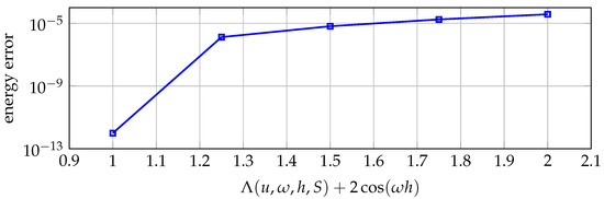
The behavior of the exponential variational integrator obtained as described above, has been examined in this work for different choices of u and the results are illustrated in Figure 1. In this figure we considered the oscillation frequency to be $\omega =1$, the time step was taken to be $h=0.01$ while the number of intermediate points was assumed to be $S=1$. For all other choices tested, the smaller energy error has been obtained when u comes out (as solution) of Equation (25).

Figure 1. Energy error for the harmonic oscillator of frequency $\omega =1$ using the exponential variational integrator for the discrete Lagrangian of (28) and for different solutions of u from Equation (25).

Even though the choice of u can be further examined, here we will consider it as coming out of Equation (25). This is especially advantageous for the extensions of the proposed techniques when they employed to treat Lagrangians of split potential functions, i.e., systems where the potential can be decomposed into several components involving different dynamical properties.

4. Family of Exponential High Order Variational Integrators

As an extension of the above method, in this section we derive a “family” of exponential high order variational integrators, following Ref. [11]. Towards this end, we split the potential energy of the Lagrangian into fast $V^f$ and slow $V^s$ terms, i.e., we write

$$L(q,\dot{q})=T\left(\dot{q}\right)-V^f\left(q\right)-V^s\left(q\right),$$

(29)

where $T\left(\dot{q}\right)$ denotes the kinetic energy of the system written as

$$T\left(\dot{q}\right)=\frac{1}{2}{\dot{q}}^{T}M\dot{q}$$

(30)

(M is a constant mass matrix) [21,22,23].

In this work, rather than using different quadrature rules to approximate the contribution of each component of the potential into the action (as done in Ref. [21]), we will follow a more general approach and we will use different number of intermediate points for the $V^f$ and $V^s$ [12,24,25]. By assuming that $S_1$ and $S_2$ represent the number of the points for the slow and fast potential, respectively, here we will restrict ourselves to choices for which $S_1<S_2$ (the choice $S_1=S_2$ creates the exponential integrators of Section 3).

Before embarking to specific simulation experiments, we should note that, after performing the discretization in (29) and adopting different quadrature rules for the two different potentials, the resulted discrete Lagrangian can be cast in the form

$$\begin{array}{c}\hfill L_d^{S_1,S_2}(q_k,q_{k+1})=h\left[\sum _{j=0}^{S_1-1}{w}_1^j\left[T\left(\dot{q}\left(t_k^j\right)\right)-V^s\left(q\left(t_k^j\right)\right)\right]-\right.\\ & \left.\sum _{j=0}^{S_2-1}{w}_2^j{V}^f\left(q\left(t_k^j\right)\right)\right],\end{array}$$

(31)

where the intermediate positions $q\left(t_k^j\right)$ and velocities $\dot{q}\left(t_k^j\right)$ may be taken from Equations (15) and (16), while the weights $w_1$ and $w_2$ could be deduced by exploiting Equation (19).

5. Numerical Examples

As representative examples, in this section we consider numerical solutions of the general N-body problem. As it is well known, the gravitational motion of an N-body system is described by a Lagrangian function of the general form [5,6]

$$L(q,\dot{q})=\frac{1}{2}\sum _{i=1}^N{m}_i{\dot{q}}_i^2+\sum _{i=1,j=1,i\ne j}^{N}G\frac{m_i{m}_j}{\left|\right|q_i-q_j\left|\right|}$$

(32)

where G stands for the gravitational constant. In the following subsections, we are going to study two special cases of the latter Lagrangian function: (i) the corresponding to the satellite solar system (where $N=3$), and (ii) the corresponding to the complete solar system (where $N=11$).

5.1. Gravitational Motion of the Satellite Solar System

The satellite solar system (also called modified solar system) consists of three bodies ($N=3$): the main (big) body and the two relatively small ones (planets) moving under the influence of their mutual gravitational attraction. For the description of this kind of planar motion, we consider masses $m_1=1$, $m_2=m_3={10}^{-2}$, initial configurations $q_1=(0,0)$, $q_2=(1,0)$, $q_3=(4,0)$ and initial velocities ${\dot{q}}_1=(0,0)$, ${\dot{q}}_2=(0,1)$, ${\dot{q}}_3=(0,0.5)$. Under these circumstances, it has been shown that the trajectories of the two planets (with respect to the main body, the Sun) are nearly circular with periods close to $2\pi$ and $14\pi$, respectively (for more details see Ref. [5]).

In order to illustrate the advanced features of the proposed method, we considered, as a next step, an additional (fourth) body a satellite of mass $m_4={10}^{-4}$ which moved rapidly around the mass $m_2$. In this way, we included in the initial system a body moving with significantly different velocity (compared to that of the planets). The Lagrange function that described the final (four-body) system was then written as

$$L(q,\dot{q})=\frac{1}{2}\sum _{i=1}^3{m}_i{\dot{q}}_i^2-V^f\left(q\right)-V^s\left(q\right),$$

(33)

where

$$V^s\left(q\right)=\sum _{i<j,(i,j)\ne (2,4)}^4\frac{m_i{m}_j}{\left|\right|q_i-q_j\left|\right|},V^f\left(q\right)=\frac{m_2{m}_4}{\left|\right|q_2-q_4\left|\right|}.$$

(34)

In order to proceed further, we chose for the satellite $m_4$ the initial position and velocity to be: $q_4=(1.01,0)$ and $p_4=(0,0)$, respectively.

Figure 2 shows the comparison of the global errors in the (four-body) system’s total energy at $t=1$ for time-step choices: $h\in \{{10}^{-4},{10}^{-2},5\times {10}^{-2}\}$, see [10]. Towards obtaining these results, we applied the proposed exponential variational integrators of Section 4 with the use of different numbers of intermediate points for the slow potential and the fast one of (34), namely $S_1$ (for the slow) and $S_2$ (for the fast). In fact, in Figure 2, the graphs correspond to the choices $S_1=3$, $S_2=3$ (blue dashed line), $S_1=3$, $S_2=5$ (red line) and $S_1=5$, $S_2=5$ (green line).

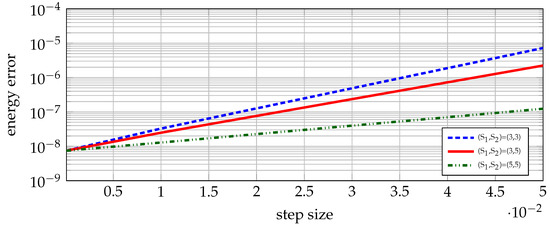
Figure 2. Modified satellite solar system. Global error for the energy error using the proposed family of exponential methods for $S_1=3$, $S_2=5$ (red line), $S_1=5$, $S_2=5$ (green line) and the ones that use $S_1=S_2=3$ (blue line).

From Figure 2, it is obvious that the the graphs derived for $S_1=S_2=3$ (blue line) were simply the standard high order variational integrator schemes of Ref. [10]. For all step sizes tested, the results obtained by increasing $S_2$ (while keeping $S_2>S_1$), showed that the energy errors became progressively smaller.

For the sake of completeness we have, in addition, tested the proposed methods with respect to their computational time consumed to obtain the same position errors. These simulated experiments showed us an interesting result which is depicted in Figure 3. As one can see, when comparing the method using $S_1=3$, $S_2=5$ (red-solid line) with the one using $S_1=5$, $S_2=5$ (green-dashed line), the latter scheme was more time consuming.

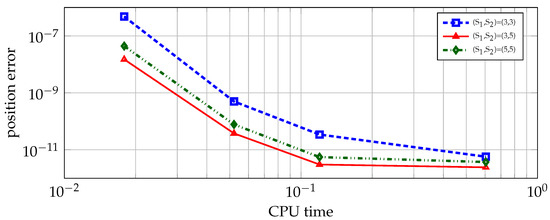
Figure 3. Position error for the modified satellite solar system an arbitrary taken time $t=1$ for the exponential integrators for $S_1=3$, $S_2=5$ (red line), $S_1=5$, $S_2=5$ (green line) and the ones that use $S_1=S_2=3$ (blue line).

5.2. The Complete Solar System (N = 11)

As a final and more complicated example, we further considered the numerical solution of the complete solar system, see [5]. This is a special case of the N-body problem for $N=11$, which consists of the nine planets of our solar system orbiting around the Sun and the Moon which is orbiting around the Earth (by adding a satellite in one of the planets, the mathematical problem becomes, obviously, more complicated). For the sake of accuracy and completeness, all initial conditions (positions and velocities) were taken from Nasa’s JPL data base.

The general N-body system can be described through the Lagrangian

$$L(q,\dot{q})=\frac{1}{2}\sum _{i=1}^N{m}_i{\dot{q}}_i^2+\sum _{i=1,j=1,i\ne j}^{N}G\frac{m_i{m}_j}{\left|\right|q_i-q_j\left|\right|},$$

(35)

for $G=2.95912208286\times {10}^{-4}$ [5]. In order to test the proposed schemes of Section 4, we split the potential of the latter Lagrangian in two terms as

$$V^s\left(q\right)=\sum _{i=1,j=1,i\ne j}^{5}G\frac{m_i{m}_j}{\left|\right|q_i-q_j\left|\right|},V^f\left(q\right)=\sum _{i=6,j=6,i\ne j}^{11}G\frac{m_i{m}_j}{\left|\right|q_i-q_j\left|\right|}.$$

(36)

Initially, we chose $S_1=3$ for the slow potential and $S_2=5$ for the fast one, and study the time evolution of the various energy-components of the system. In Figure 4 we plot the various terms of the Lagrangian (32), namely the potential (black dashed line) and the kinetic energy (blue dashed line) components. Additionally, we plot the calculated total energy (red line), which was expected to remain constant throughout the integration process. In this simulated experiment, the time step was chosen to be equal to 2 days (a relatively long time step was required to keep on truck fast orbiting objects, the Moon in our example). In order to assess the accuracy and stability of the method, all the results presented were obtained for ${10}^6$ days (a rather long time). The good and stable behavior of the method is evident from Figure 4.

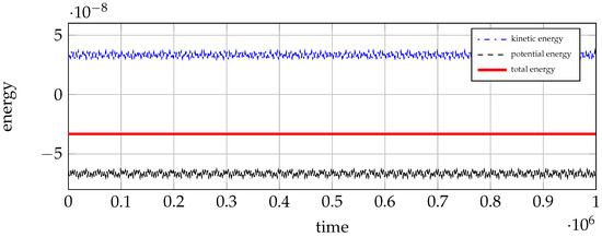
Figure 4. Kinetic, potential and total energy evolution for the numerical integration of the solar system problem for 1 million days, using family of exponential integrators with $S_1=3$, $S_2=5$ and $h=2$ days.

Finally, the global errors for the total energy of the system at $t=1000$ for time steps $h\in \{0.5,1,2.5,5\}$ days were compared. In Figure 5 we show the results obtained by applying the above schemes choosing $S_1=3$, $S_2=5$ (red line), $S_1=5$, $S_2=5$ (black line) as well as those obtained with $S_1=S_2=3$ (blue line). From all cases tested, it is apparent that the smaller energy errors found corresponded to choices for which $S_2>S_1$, a conclusion which is in agreement with the findings of the previous simulated experiment.

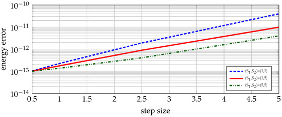
Figure 5. Solar system. Global error for the energy error using the proposed family of exponential methods for $S_1=3$, $S_2=5$ (red line), $S_1=5$, $S_2=5$ (green line) and the ones that use $S_1=S_2=3$ (blue line).

It is worth noting that the above numerical examples demonstrated the same errors in energy by using $S_2>S_1$ compared to $S_1=S_2=3$ for approximately $15\%$ longer time step. This implies that, the proposed schemes had excellent energy preserving properties compared to standard schemes.

Before closing, it should be stressed that the proposed method is based on the high order variational integrator schemes of Refs. [10,11] that have been properly deduced to address nonlinear phenomena and specifically stiff problems in which some physical observable is varying with exceptionally high-frequency. The resulted discrete equations for such systems, may be viewed as coming out of a finite-dimensional Hamiltonian with special symmetry properties. Subsequently, these discrete equations are time-integrated with the aid of the new variational integrators. The latter advanced schemes possess enhanced numerical stability properties in the nonlinear regime (see also Refs. [16,25] where the above exponential variational methods with at least one intermediate point have been proven to be unconditionally stable).

6. Conclusions

In the present work, we developed a special type of numerical integration schemes which are based on the discretization of the Hamilton’s principle. They are appropriate to be applied in systems that are described via an energy functional in which its potential component may be separated into various parts with strongly different dynamics. Interesting simulation problems of this kind appear in N-body gravitational systems, where their mutual interactions can be written as mentioned before and may lead to extremely stiff potential terms that force the solution to oscillate on a very small time scale.

The proposed high order numerical integrators rely on exponential functions entering the discrete action and on the application of different quadrature rules to the different component potentials. In this way, the derived integrators respect the geometric characteristics of the system while at the same time show great accuracy, convergence and short computational time compared to standard schemes.

References

- Engquist, B.; Fokas, A.; Hairer, E.; Iserles, A. Highly Oscillatory Problems; Cambridge University Press: Cambridge, UK, 2009. [Google Scholar]
- Wendlandt, J.; Marsden, J.E. Mechanical integrators derived from a discrete variational principle. Physica D 1997, 106, 223–246. [Google Scholar] [CrossRef] [Green Version]
- Kane, C.; Marsden, J.E.; Ortiz, M. Symplectic-energy-momentum preserving variational integrators. J. Math. Phys. 2001, 40, 3353–3371. [Google Scholar] [CrossRef] [Green Version]
- Marsden, J.E.; West, M. Discrete mechanics and variational integrators. Acta Numer. 2001, 10, 357–514. [Google Scholar] [CrossRef] [Green Version]
- Hairer, E.; Lubich, C.; Wanner, G. Geometric numerical integration illustrated by the Störmer-Verlet method. Acta Numer. 2003, 12, 399–450. [Google Scholar] [CrossRef] [Green Version]
- Leimkuhler, B.; Reich, S. Simulating Hamiltonian dynamics. In Cambridge Monographs on Applied and Computational Mathematics; Cambridge University Press: Cambridge, UK, 2004. [Google Scholar]
- Ober-Blöbaum, S. Galerkin variational integrators and modified symplectic Runge-Kutta methods. IMA J. Numer. Anal. 2017, 37, 375–406. [Google Scholar] [CrossRef]
- Ober-Blöbaum, S.; Saake, N. Construction and analysis of higher order Galerkin variational integrators. Adv. Comput. Math. 2015, 41, 6. [Google Scholar] [CrossRef]
- Campos, C.; Junge, O.; Ober-Blöbaum, S. Higher order variational time discretization of optimal control problems. arXiv 2012, arXiv:1204.6171. [Google Scholar]
- Kosmas, O.T.; Leyendecker, S. Variational integrators for orbital problems using frequency estimation. Adv. Comput. Math. 2019, 45, 1–21. [Google Scholar] [CrossRef] [Green Version]
- Kosmas, O.T.; Leyendecker, S. Family of higher order exponential variational integrators for split potential systems. J. Phys. Conf. Ser. 2015, 574, 012002. [Google Scholar] [CrossRef]
- Kosmas, O.T.; Vlachos, D.S. Exponential Variational Integrators Using Constant or Adaptive Time Step. In Discrete Mathematics and Applications; Springer: Cham, Switzerland, 2020; pp. 237–258. [Google Scholar]
- Kosmas, O.T. On the stability of exponential variational integrators for multibody systems with holonomic constraints. J. Phys. Conf. Ser. 2020, 1730, 012139. [Google Scholar] [CrossRef]
- Kosmas, O.T. Exponential variational integrators for the dynamics of multibody systems with holonomic constraints. J. Phys. Conf. Ser. 2019, 1391, 012170. [Google Scholar] [CrossRef]
- Kosmas, O.T.; Papadopoulos, D.; Vlachos, D. Geometric derivation and analysis of multi-symplectic numerical schemes for differential equations. Comput. Math. Var. Anal. 2020, 159, 207–226. [Google Scholar]
- Kosmas, O.T.; Leyendecker, S. Stability analysis of high order phase fitted variational integrators. In Proceedings of the 11th World Congress on Computational Mechanics (WCCM XI), 5th European Conference on Computational Mechanics (ECCM V), 6th European Conference on Computational Fluid Dynamics (ECFD VI), Barcelona, Spain, 20–25 July 2014; Volume 1389, pp. 865–866. [Google Scholar]
- Deuflhard, P. A study of extrapolation methods based on multistep schemes without parasitic solutions. Z. Angew. Math. Phys. 1979, 1979 30, 177–189. [Google Scholar] [CrossRef]
- García-Archilla, B.; Sanz-Serna, M.J.; Skeel, R.D. Long-time-step methods for oscillatory differential equations. SIAM J. Sci. Comput. 1999, 20, 930–963. [Google Scholar] [CrossRef] [Green Version]
- Gautschi, W. Numerical integration of ordinary differential equations based on trigonometric polynomials. Numer. Math. 1961, 3, 1. [Google Scholar] [CrossRef]
- Hochbruck, M.; Lubich, C.; Selfhofer, H. Exponential integrators for large systems of differential equations. SIAM J. Sci. Comput. 1998, 19, 1552–1574. [Google Scholar] [CrossRef] [Green Version]
- Stern, A.; Grinspun, E. Implicit-explicit integration of highly oscillatory problems. SIAM Multiscale Model. Simul. 2009, 7, 1779–1794. [Google Scholar] [CrossRef] [Green Version]
- Reich, S. Backward error analysis for numerical integrators. SIAM J. Numer. Anal. 1999, 36, 1549–1570. [Google Scholar] [CrossRef] [Green Version]
- Leok, M.; Zhang, J. Discrete Hamiltonian variational integrators. IMA J. Numer. Anal. 2011, 31, 1497–1532. [Google Scholar] [CrossRef] [Green Version]
- Kosmas, O.T.; Vlachos, D.S. A space-time geodesic approach for phase fitted variational integrators. J. Phys. Conf. Ser. 2016, 738, 012133. [Google Scholar] [CrossRef]
- Kosmas, O.T.; Vlachos, D.S. Error Analysis Through Energy Minimization and Stability Properties of Exponential Integrators. Nonlinear Anal. Glob. Optim. 2021, 295, 295–307. [Google Scholar]
Publisher’s Note: MDPI stays neutral with regard to jurisdictional claims in published maps and institutional affiliations. |
© 2021 by the author. Licensee MDPI, Basel, Switzerland. This article is an open access article distributed under the terms and conditions of the Creative Commons Attribution (CC BY) license (https://creativecommons.org/licenses/by/4.0/).