Article

Modified Polynomial Chaos Expansion for Efficient Uncertainty Quantification in Biological Systems

1
Department of Chemical & Biomolecular Engineering, Clarkson University, Potsdam, NY 13699, USA
2
Department of Industrial, Manufacturing & Systems Engineering, Texas Tech University, Lubbock, TX 79409, USA
*
Author to whom correspondence should be addressed.
Appl. Mech. 2020, 1(3), 153-173; https://doi.org/10.3390/applmech1030011
Submission received: 12 May 2020 / Revised: 11 August 2020 / Accepted: 20 August 2020 / Published: 22 August 2020

Abstract

:
Uncertainty quantification (UQ) is an important part of mathematical modeling and simulations, which quantifies the impact of parametric uncertainty on model predictions. This paper presents an efficient approach for polynomial chaos expansion (PCE) based UQ method in biological systems. For PCE, the key step is the stochastic Galerkin (SG) projection, which yields a family of deterministic models of PCE coefficients to describe the original stochastic system. When dealing with systems that involve nonpolynomial terms and many uncertainties, the SG-based PCE is computationally prohibitive because it often involves high-dimensional integrals. To address this, a generalized dimension reduction method (gDRM) is coupled with quadrature rules to convert a high-dimensional integral in the SG into a few lower dimensional ones that can be rapidly solved. The performance of the algorithm is validated with two examples describing the dynamic behavior of cells. Compared to other UQ techniques (e.g., nonintrusive PCE), the results show the potential of the algorithm to tackle UQ in more complicated biological systems.

1. Introduction

Models are often used to describe biological systems, for which parameters are often considered as fixed constants [1,2]. However, model parameters cannot be known with certainty due to model calibration with noisy data or the time-varying nature of a dynamic system. The main objective of uncertainty quantification (UQ) is to study the impact of uncertainty (e.g., the variation in model parameters) on model predictions [1,3,4,5,6], which is vital to assess the trustworthiness of model predictions for process design and performance evaluation [2,4,7,8].
There are several ways for UQ and the most popular tool is the sampling-based Monte Carlo (MC) simulations [9]. Typically, MC predicts uncertainty in model predictions by generating samples from the distribution of parametric uncertainty and by running the model with each sample. Although MC is methodically simple, the UQ accuracy is affected by the total number of samples, especially when the model has complex forms such as nonpolynomial terms [9]. In this case, many samples are required to ensure UQ accuracy, which may greatly increase the computational cost.
Compared to MC, polynomial chaos expansion (PCE) [10,11] has gained a growing interest in engineering and scientific problems [2,12,13]. For example, it was used to predict dynamic behaviors of the electrochemical flow in a microfluidic system [13] and to quantify uncertainty in biochemical systems [12] and epidemic models [2]. The key of PCE is to determine the PCE coefficients for both parametric uncertainty and model predictions. The PCE coefficients of parametric uncertainty can be obtained with parameter estimation [14], while the coefficients of model predictions have to be calculated based on the coefficients of parametric uncertainty. Depending on how the PCE coefficients of model outputs are calculated, the PCE-based UQ can be categorized into intrusive and nonintrusive approaches [10,15,16].
For the intrusive method, the stochastic Galerkin (SG) projection is required to compute PCE coefficients of model predictions, which often involves calculating high-dimensional integrals [10]. Note that there are several algorithms to facilitate the calculation of SG without directly evaluating high-dimensional integrals, which include the pseudo-spectral construction and integration method by exploiting the orthogonal property of the polynomial basis. Details of these intrusive approaches for SG can be found in References [16,17]. However, in this work we will focus on the implementation of SG with direct evaluation of high-dimensional integrals to simplify the procedures required to calculate PCE coefficients of model predictions.
While the efficiency of the SG-based UQ was verified in several applications in terms of UQ accuracy and computational time [14,15,16,18,19], the calculation of PCE coefficients with the SG projection can be challenging, especially when the model involves many uncertainties and nonpolynomial terms [10,17]. In this case, it may be computationally prohibitive to compute the PCE coefficients of model predictions, especially when evaluating high-dimensional integrals is required. To address this, we have developed an algorithm to convert a high-dimensional integral in SG into a few lower-dimensional ones [20,21], using the generalized dimension reduction method (gDRM) [22]. This approach can efficiently deal with a moderate number of uncertainties. However, we found that the computational efficiency can be reduced as the total number of uncertainties increases [21]. Motivated by this, in this work we modify the existing algorithm by integrating the gDRM and numerical approximation techniques (e.g., Gauss quadrature [23]) with the SG projection to reduce computational cost. It is worth mentioning that the approach appears to be similar to the analysis of variance (ANOVA) expansions [24], for which the dimensionality of the problem can be reduced and sampling methods are often used to evaluate the integrals. However, the approach in this work treats each dimension equally, while the ANOVA expansion identifies the most effective dimension of the problem [24].
Another approach for the PCE-based UQ is stochastic collocation (SC) [10], which is hereafter referred to as nonintrusive discrete projection (NIDP). The application of SC is methodically similar to MC [10], which requires to generate samples of uncertainty. These samples are often referred to as collocation points, which play an essential role in the NIDP-based UQ. The most popular technique to generate collocation points is the full tensor product (NIDP-FT) but as the number of uncertainties increases, the total number of required collocation points grows significantly. This increases the computational time to compute the PCE coefficients of model predictions, which is recognized as the curse of dimensionality [10,25]. To reduce computational time, a sparse grid method (NIDP-SP) can be used to generate fewer collocation points [26,27]. For algorithm verification, the UQ approach proposed in this work will be compared to NIDP-SP due to its computational efficiency [28,29,30].
In summary, our contribution is to couple the gDRM and quadrature rules with the SG to improve the performance of the PCE-based UQ method and discuss the efficiency of the method by comparing the results to other methods in terms of UQ accuracy and computational time under a large number of uncertainties. This paper is organized as follows. In Section 2, we present a brief description of PCE and provide an overview of the proposed UQ method. Section 3 provides a detailed comparison among different algorithms with three examples—a nonlinear algebraic case study, the interaction between tumor and normal cells [31] and phase transitions of yeast cells [32]. The conclusions are summarized in Section 4.

2. Background and Methodology

2.1. Polynomial Chaos Expansion (PCE) for UQ

Suppose a dynamic system is described with nonlinear ordinary differential equations (ODE) over a given time period ( t 0 ,   t p ] as in:
x ˙ = g ( t , u , p , x ) , t ( t 0 , T ] ,
where x is the model prediction with the initial conditions x 0 at t = t 0 and u is a vector of fixed model parameters. Further, p is a vector to define parametric uncertainties, for which p = ( p i = 1 ,   ,   p i = N ) N and N indicates the total number of parametric uncertainties. In this work, we assume each parameter p i in p to be independent and identically distributed, which will be described with a prior given PDF using a random variable θ i as in:
p i = p i ( θ i ) ,
where θ i represents the i th random variable to describe the PDF of p i from the Wiener-Askey scheme [33]. Following this, each parametric uncertainty in Equation (2) is rewritten as in Reference [10]:
p i ( θ i ) = k = 0 P p ¯ i , k ψ k ( θ i ) ,
where { p ¯ i , k } denote the PCE coefficients of the i th parametric uncertainty p i [10,34] and P is the polynomial order that determines the number of terms required to approximate the uncertainty. In addition, { ψ k ( θ i ) } are the orthogonal polynomial basis functions, which should be selected appropriately depending on the PDF of p i . For instance, Hermite polynomial basis can be used to describe a normally distributed uncertainty [11]. For other distributions such as uniform distribution, their corresponding polynomial basis functions can be found in the literature [10].
Since the model response is affected by uncertainty, the resulting output can be approximated with a spectral expansion of random variables, that is, θ = ( θ 1 , , θ i , , θ N ) as in [10,34]:
x ( t , θ ) = m = 0 M x ¯ m ( t ) Ψ m ( θ ) ,
where { x ¯ m } are PCE coefficients of predictions and Ψ m ( θ ) are the orthogonal multivariate polynomial functions computed from polynomial basis function { ψ k ( θ i ) } with respect to each uncertainty p i [25]. In Equations (3) and (4), a finite number of terms, P + 1 and M + 1 , including zeroth terms, are used. If the total number of uncertainties is N and the polynomial order of each uncertainty is P , the number of terms of model prediction ( M + 1 ) is calculated as in [17]:
M + 1 = ( N + P ) ! P ! N ! .
The PCE coefficients of uncertain parameters can be calibrated with the prior information of the PDF, whereas the PCE coefficients of model responses in Equation (4), { x ¯ m } , have to be calculated with a stochastic Galerkin (SG) projection by substituting Equations (3) and (4) into Equation (1) and by projecting Equation (1) onto each of the polynomial basis functions in PCE theory, { Ψ m } , as defined in [10]:
x ˙ ( t , θ ) ,   Ψ m ( θ ) = g ( t , u , p ( θ ) , x ( t , θ ) ) ,   Ψ m ( θ ) ,   m { 0 ,   ,   M } ,
where · is the inner product operator. The SG projection in Equation (6) calculates the PCE coefficients of model prediction x and converts Equation (1) into a few coupled deterministic equations that are functions of the PCE coefficients of x . Specifically, the inner product between two functions in Equation (6) can be mathematically defined as in [10]:
φ ( θ ) , φ ( θ ) = N φ ( θ ) , φ ( θ ) W ( θ ) d θ ,
where the multivariate integration in Equation (7) is solved over the random domain N determined by θ ; and W ( θ ) is a predefined weight function described by the joint PDFs of θ , which can be chosen from the Wiener-Askey framework [10].
When the PCE coefficients of x are available, uncertainty in x , originating from uncertainty in p , can be approximated analytically. For instance, the mean value of output x can be estimated with the first PCE coefficient, x ¯ m = 0 in Equation (4) and other higher-order PCE coefficients ( x ¯ m 0 ) can be used to estimate other statistical moments such as the variance around the mean value of x [10].
The calculation of PCE coefficients { x ¯ m } in Equation (4), can be further defined as in [10]:
x ¯ m ( t ) = x ( t , θ ) ,   Ψ m ( θ ) Ψ m 2 ( θ ) = 1 γ m N x ( t , θ ) Ψ m ( θ ) W ( θ ) d θ ,
where γ m = E [ Ψ m 2 ] and E [ · ] here represents expectation. Although the SG projection-based UQ has been shown to be computationally effective over a wide range of applications [14,15,18,19], the calculation of PCE coefficient of model output x with Equation (8) is not trivial, especially when the model involves nonpolynomial functions and a large number of uncertainties [17,28]. For example, the calculation of Equation (8) can be computationally demanding as discussed in Section 3.
To address this issue, the UQ algorithm to combine the generalized dimension reduction method (gDRM or S -variate DRM) with PCE will be used to calculate high-dimensional integrals in the inner product of SG projection. This algorithm approximates a high-dimensional integral with several lower-dimensional ones that involve at most S -variables. For instance, the bivariate DRM (BiDRM and S = 2 ) estimates an N -dimensional integral with several one- and two-dimensional integrals [22]. For clarity, the approximation procedures are described in Section 2.2.

2.2. Modified gDRM-Based PCE for UQ

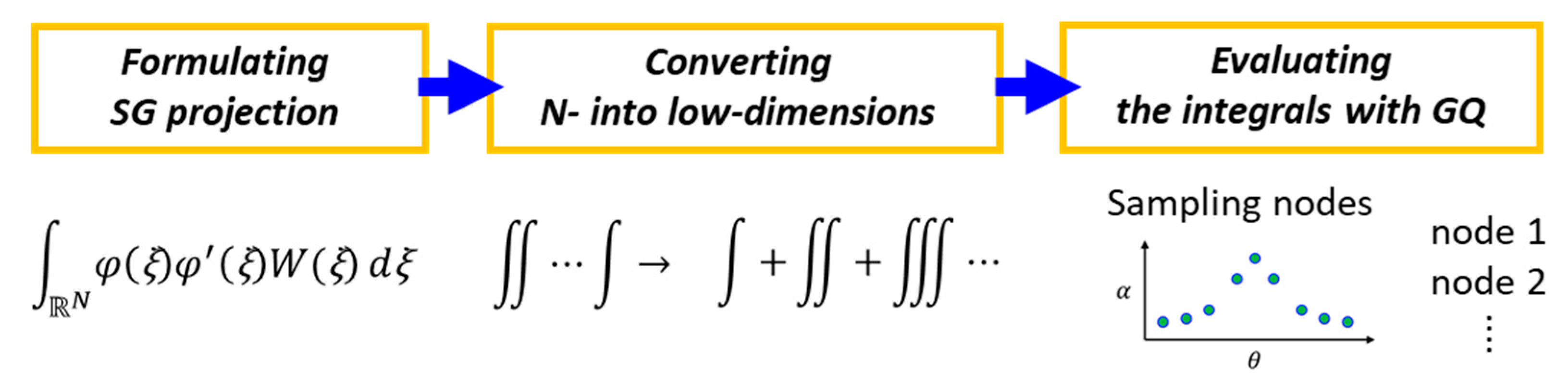
2.2.1. Dimension Reduction Based Stochastic Galerkin Projection

To solve PCE coefficients { x ¯ m } , the key is to calculate the multivariate integral in Equation (8), resulting from the inner product of SG. For simplicity, let assume y ( θ ) can be defined as y ( θ ) = x ( t , θ ) Ψ m ( θ ) at a specific time point t in Equation (8) and suppose y ( θ ) is a continuous and differentiable function. In this way, the integral in Equation (8) can be redefined as in [22]:
E [ y ( θ ) ] = N y ( θ ) W ( θ ) d θ ,
where E is an expectation operator. Following the definition of gDRM [22], each coefficient in Equation (8) can be computed as in [21]:
x ¯ m ( t ) = 1 γ m E [ y ( θ ) ] 1 γ m r = 0 S ( 1 ) r ( N S + r 1 r ) E [ y S r ] ,
where each term in Equation (10), that is, y S r can be further defined as in [22]:
y S r = ω 1 < ω 2 < < ω S r y ( 0 , , 0 , θ ω 1 , 0 , , 0 , θ ω 2 , 0 , , 0 , θ ω S r , 0 ) ,
where ω 1 , ω 2 , , ω S r =   1 ,   2 , ,   N . Note that for the last term in the summation of Equation (11), S = r and y S r can be defined as y 0 = y ( 0 ) by setting the mean values of all random variables θ to 0. Based on Equation (10), the PCE coefficients of x can be rapidly calculated, even if the model of a system involves nonpolynomial terms. For brevity, details are not given here, which can be found in our previous works [20,21]. An example of the trivariate DRM (TriDRM), that is, S = 3 in gDRM, is given for clarity. For TriDRM, each term E [ y S r ] in Equation (10) is determined as follows.
E [ y 0 ] = y ( 0 ) = y 0 = y ( 0 , ,   0 )
E [ y 1 ] = ω 1 E [ y ( 0 , , 0 , θ ω 1 , 0 ,   , 0 ) ] = ω 1 { y ( 0 , , 0 , θ ω 1 , 0 ,   , 0 ) W ( θ ω 1 ) d θ ω 1 }
E [ y 2 ] = ω 1 < ω 2 E [ y ( 0 , , 0 , θ ω 1 , 0 , , 0 , θ ω 2 , 0 , , 0 ) ] = ω 1 < ω 2 { y ( 0 , , 0 , θ ω 1 , 0 , , 0 , θ ω 2 , 0 , , 0 ) W ( θ ¯ ) d θ ¯ }
E [ y 3 ] = ω 1 < ω 2 < ω 3 E [ y ( 0 , , 0 , θ ω 1 , 0 , , 0 , θ ω 2 , 0 , , 0 , θ ω 3 , 0 ) ] = ω 1 < ω 2 < ω 3 { y ( 0 , , 0 , θ ω 1 , 0 , , 0 , θ ω 2 , 0 , , 0 , θ ω 3 , 0 ) W ( θ ¯ ) d θ ¯ } .
As seen, each term in Equation (10) is defined with at most three random variables, resulting in several lower-dimensional integrals. Specifically, Equation (12) is calculated by setting θ to 0 and Equations (13) to (15) are defined as summations of ( N 1 ) , ( N 2 ) and ( N 3 ) integrals, involving one-, two- and three-variables, respectively [22]. In addition, θ ¯ in Equations (14) and (15) are defined with a subset of variables selected from θ . For example, θ ¯ = { θ ω 1 , θ ω 2 } in Equation (14), θ ¯ = { θ ω 1 , θ ω 2 , θ ω 3 } in Equation (15) and W ( θ ¯ ) is the joint PDF of θ ¯ .
In summary, as in Equations (13) to (15), N one-dimensional integrals are required to estimate E [ y 1 ] , while E [ y 2 ] and E [ y 3 ] are computed with ( N 2 ) two- and ( N 3 ) three-dimensional integrals, respectively. In this way, a high-dimensional integral that is required to calculate each PCE coefficient as in Equation (8) can be approximated with a few lower-dimensional ones.
As discussed in Section 3 below, this approach is computationally efficient when the number of uncertainties is small. However, we found that the computational cost increases greatly, when the number of uncertainties increases. For example, when the number of uncertainties is 20 (i.e., 20 random variables are required to define uncertainties) and TriDRM (i.e., S = 3 in Equation (10)) is used to calculate PCE coefficients of model outputs, in total 1140 three-, 190 two- and 20 one-dimensional integrals should be computed. For such a case, it can be computationally prohibitive to calculate PCE coefficients. To attenuate the computational cost, we will integrate sampling-based quadrature rules with the gDRM-based PCE to numerically estimate these low-dimensional integrals. The modified gDRM-based PCE method is discussed below.

2.2.2. Modified gDRM-Based PCE Sing the Dimension Reduction and Quadrature Rules

The key of the modified gDRM-based PCE method is to approximate the integrals involved in Equation (10) (i.e., E [ y S r ] ) with quadrature rules. For algorithm clarification, Gaussian quadrature rules [23,35] will be used in this work; but other multidimensional integral approximations can be also applied. The calculation of PCE coefficients with gDRM in Equation (10) can be redefined as in:
x ¯ m ( t ) = 1 γ m r = 0 S ( 1 ) r ( N S + r 1 r ) E [ y ˜ S r ] ,
where E [ y ˜ S r ] represents that each lower-dimensional integral in Equation (10) is estimated with the Gaussian quadrature rules. For each random variable, for example, θ ω 1 in Equation (13), a one-dimensional quadrature rule can be constructed as in:
y ( 0 , , 0 , θ ω 1 , 0 ,   , 0 ) W ( θ ω 1 ) d θ ω 1 q 1 = 1 Q 1 y ( 0 , , 0 , θ ω 1 q 1 , 0 ,   , 0 ) · α ω 1 q 1 ,
where { θ ω 1 q 1 ,   α ω 1 q 1 } q 1 = 1 Q 1 represent a set of integral evaluation points (i.e., θ ω 1 q 1 ) and their related weights (i.e., α ω 1 q 1 ) that will be used to estimate the one-dimensional integral (i.e., ω 1 = 1, 2, , N ) in Equation (13). Note that evaluation points and their weights have to be carefully selected by considering the PDFs of random variables (e.g., θ ω 1 ) to ensure the exponential convergence. For example, Gauss-Hermite quadrature is the best choice for normal distribution [23,35]. It is also worth mentioning that Gauss quadrature rule provides an exact result when the polynomial degree of the integrand is less than 2 Q 1 1 , where Q 1 is the number of evaluation points [16,23].
For multidimensional integrals (i.e., S r 2 in Equations (14) and (15)), we will use full tensor evaluation points, constructed by tensor product with one-dimensional quadrature rules of each individual random variable. The full tensor evaluation is used in this work, since these integrals resulting from the gDRM step only involve a few random variables. Thus, the approximation of a multidimensional integral ( N ) can be evaluated in real-time. However, it is important to point out that when high-dimensional integrals are yielded from the gDRM step, such as when S r 6 , sparse grids with a smaller number of evaluation points can be used to reduce the computational cost for approximating integrals in Equation (10) [10].
As an example, Equations (18) to (20) show the calculations of these lower-dimensional integrals in Equation (16), when TriDRM-PCE is used to calculate the PCE coefficients of outputs. In this case, the approximation of these integrals E [ y ˜ S r ] in Equation (16), that is, N one-dimensional, ( N 2 ) two-dimensional and ( N 3 ) three-dimensional integrals in Equations (13) to (15), can be calculated with the quadrature rules as in:
E [ y ˜ 1 ] ω 1 { q 1 = 1 Q 1 y ( 0 , , 0 , θ ω 1 q 1 , 0 ,   , 0 ) · α ω 1 q 1 }
E [ y ˜ 2 ]   ω 1 < ω 2 { q 1 = 1 Q 1 q 2 = 1 Q 2 y ( 0 , , 0 , θ ω 1 q 1 , 0 , , 0 , θ ω 2 q 2 , 0 , , 0 ) · ( α ω 1 q 1 α ω 2 q 2 ) }
E [ y ˜ 3 ]   ω 1 < ω 2 < ω 3 { q 1 = 1 Q 1 q 2 = 1 Q 2 q 3 = 1 Q 3 y ( 0 , , 0 , θ ω 1 q 1 , 0 , , 0 , θ ω 2 q 2 , 0 , , 0 , θ ω 3 q 3 , 0 ) · ( α ω 1 q 1 α ω 2 q 2 α ω 3 q 3 ) } ,
where Q i is the total number of quadrature evaluation points θ ω i q i , α ω i q i is the corresponding weights of each evaluation point and i is the index of random variables in the gDRM-based PCE. To estimate a multidimensional integral with quadrature rules, the same number of evaluation points and weights are used for each random variable. Thus, based on the tensor product rules, the number of evaluation points required to estimate a multidimensional integral is defined as Q = i = 1 S r Q i = Q i S r [23,35]. We found that the estimation of lower-dimensional integrals (e.g., one-, two- and three-dimensional integrals) with Gaussian-quadrature points can significantly reduce the computational time to compute PCE coefficients, which will be discussed with three examples in Section 3.

2.2.3. Modified gDRM-Based PCE Using the Dimension Reduction and Quadrature Rules

A schematic of the modified gDRM-based PCE-based UQ is shown in Figure 1, which integrates the gDRM and quadrature rules to quickly solve the high-dimensional integral involved in the SG step. To calculate each PCE coefficient of model output in Equation (4), the inner product of the SG projection will yield a high-dimensional integral as in Equation (8). To alleviate the computational burden, gDRM is used to convert a high-dimensional integral in the SG projection into several low-dimensional ones. Since we found a large number of lower-dimensional integrals have to be calculated when the number of uncertainties is large, sampling-based quadrature rule (i.e., Gaussian Quadrature) is used to calculate the lower-dimensional integrals. This will calculate the PCE coefficients of model outputs in real-time, which can be used to quickly assess the impact of uncertainty on model predictions.

2.3. Sampling-Based Nonintrusive Discrete Projection (NIDP)

The SC-based nonintrusive approach is another way to deal with nonpolynomial functions and a large number of uncertainties. As a discrete projection [10], the unknown PCE coefficients of x , { x ¯ m } , are approximated with repetitive simulations. The model response x in Equation (4) can be described as in [10]:
x z ( t , ϑ ) = m = 0 M z ¯ m ( t ) Ψ m ( ϑ ) ,
where ϑ is a vector of random variables, ϑ =   ( ϑ 1 , , ϑ i , , ϑ N ) , as described with θ in Equation (4) and the PCE coefficients { z ¯ m } at each time point t in Equation (21) are calculated as in [10]:
z ¯ m ( t ) = 1 γ m j = 1 Q x ( t ,   ϑ j ) Ψ m ( ϑ j ) λ j ,
where Q is the number of collocation points ϑ j = ( ϑ 1 j ,   ,   ϑ N j ) to estimate { z ¯ m } , { λ j } are the corresponding weights of collocation points and j is an index to define the j th point and its weight generated in a random space characterized by N random variables.
To calculate the PCE coefficients in Equation (22), collocation points must be appropriately chosen so that the difference between Equation (22) and the spectral projection in Equation (8) is minimized [10]. The most popular way to select collocation points in Equation (22) is to use the sampling points generated by the Gaussian quadrature rules [23,35], which are related to the PDFs of random variables. For example, Gauss-Hermite quadrature rules are one way to select collocation points for normally distributed uncertainty [23,35].
Suppose each term in the summation in Equation (22) can be defined as f ( ϑ j ) = x ( t ,   ϑ j ) Ψ m ( ϑ j ) for simplicity. For each random variable, that is, ϑ i , a one-dimensional integration rule is constructed as in [28]:
U i n i j = 1 n i f ( ϑ i j ) · λ i j ,
where the set of collocation points used in Equation (23) is represented as [28]:
𝓞 i 1 = ( ϑ i 1 , , ϑ i n i ) .
Once a one-dimensional quadrature rule for each random variable is determined as in Equations (23) and (24), the next step is to formulate collocation points from a random space defined with N independent random variables. The simplest way to generate collocation points is to use a full tensor product grid, which is given as in [28]:
U Q [ f ] ( U 1 n 1 U N n N ) [ f ] = j 1 = 1 n 1 j N = 1 n N f ( ϑ 1 j 1 , , ϑ N j N ) · ( λ 1 j 1 λ N j N ) .
As seen, the full tensor grid to calculate a high-dimensional integral only requires tensor products of one-dimensional quadrature rules. Thus, the collocation points are mathematically given as: 𝓞 N = O n 1 1 × × O n N 1 [10]. However, the full tensor product can be computationally intensive when many uncertainties are considered. In this case, it may require many collocation points to obtain accurate UQ results. For example, when N uncertainties and n i collocation points are used for each uncertainty, the total collocation points Q of the full tensor grid can be defined as Q = i = 1 N n i [23,35]. As seen, the total number of collocation points for UQ grows greatly, when the number of uncertainties increases.
Alternatively, a sparse grid using the Smolyak algorithm [26,27] can significantly decrease the number of collocation points. The Smolyak algorithm is based on linear combinations of tensor product construction, which only needs a subset of the full tensor product grids in Equation (25). Details of the sparse grid constructed by the Smolyak algorithm can be found in References [26,27,28]. For brevity, the construction of the sparse grid with the Smolyak algorithm is given as in [27]:
U Q [ f ] = w + 1 | i | w + N ( 1 ) w + N | i | · ( N 1 w + N | i | ) · ( U i 1 U i N ) ,
where | i | = i 1 + + i N and w is a level of approximation, which is the parameter to decide the number of tensor product elements required to construct the Smolyak grid. The collocation points with sparse grids to evaluate Equation (26) are given as in [28]:
𝓞 N = w + 1 | i | w + N ( O i 1 1 × × O i N 1 ) .
As seen in Equation (27), the total number of collocation points 𝓞 N can be greatly decreased, when the nested condition is satisfied for collocation points in each dimension O i 1 so that O i , w 1 O i , w + 1 1 [28]. More details about the nested property of sparse grids can be found in the literature [26,27]. Since our objective is to develop an efficient UQ method to deal with a large number of uncertainties ( N 6 ), the Smolyak algorithm based sparse grid method will be used to show the efficiency of our algorithm in terms of UQ accuracy and computational efficiency.

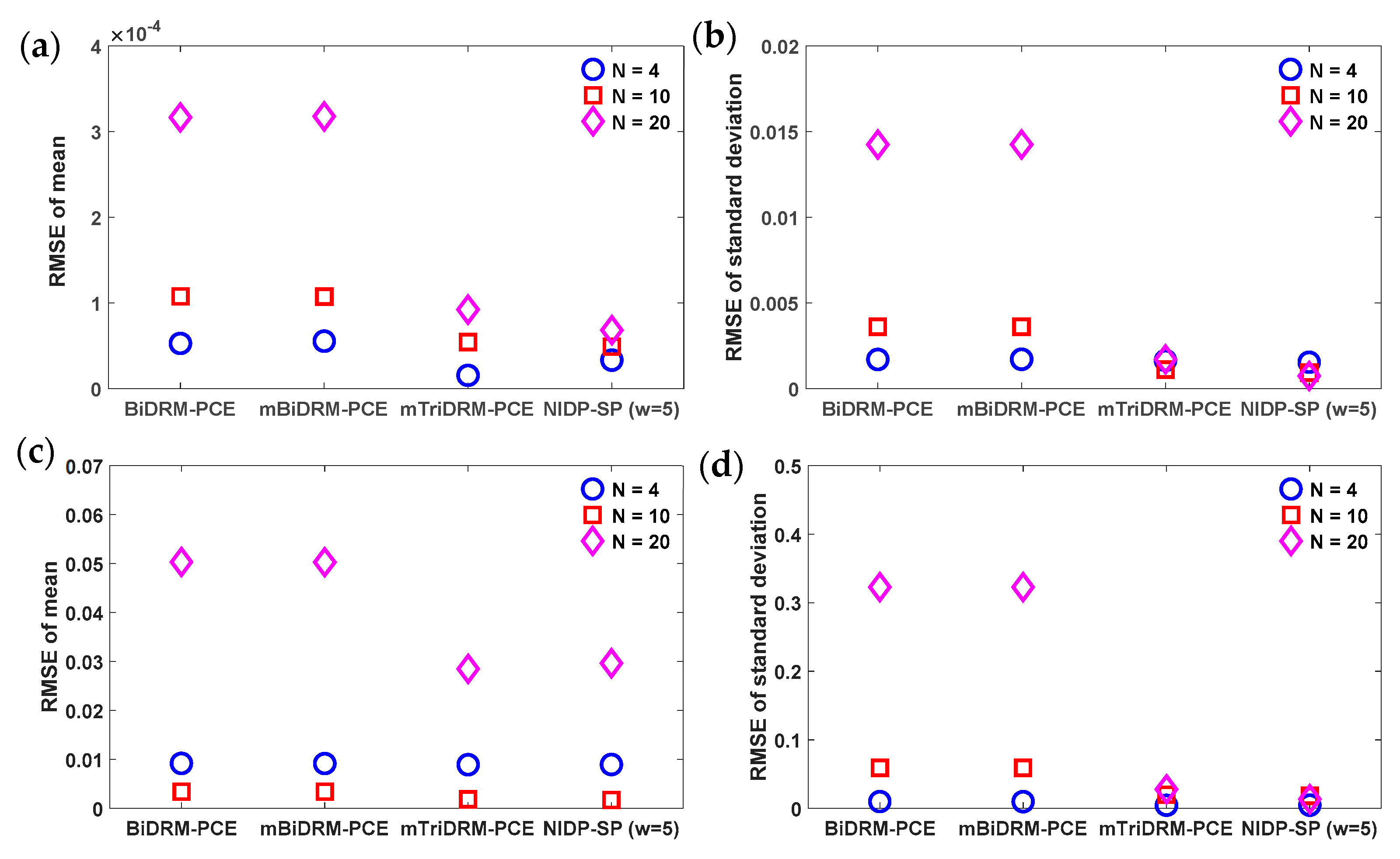
2.4. Root-Mean-Square Error (RMSE) to Evaluate UQ Accuracy

For algorithm comparison, the root-mean-square error (RMSE) is used to compare UQ errors of the proposed modified gDRM-based PCE method and other algorithms, which is defined as in [36]:
R M S E = 1 H h = 1 H [ l ( h ) l r e f ( h ) ] 2 ,
where l denotes either mean or standard deviation of model predictions obtained with different UQ methods and l r e f is a reference of the corresponding statistical moments calculated with MC. In Equation (28), h is an index defining UQ results at a specific time point h of simulations and the total number of time instants used to calculate the RMSE is defined as H .

3. Numerical Examples

Three case studies were used to compare the performance of different UQ methods in terms of computational efficiency and UQ accuracy. A nonlinear algebraic problem was used as a benchmark example to compare the accuracy of the proposed modified gDRM-based PCE method to other existing algorithms. Two additional examples, a biochemical process in the conjoint tumor-normal cell populations [31] and the G2 to Mitosis transition phase for the fission yeast [32], were further used to show the accuracy and computational efficiency, when dealing with complex and nonlinear systems that involve many uncertainties. For each example, RMSE in Equation (28) was calculated and the computational time was measured in terms of central processing unit (CPU) time with an office desktop (Core i5-8400 CPU at 2.80 GHz).

3.1. Example 1: Nonlinear Algebraic Problems

The UQ accuracy of the proposed algorithm in this work is first compared to other approaches using a nonlinear algebraic example, for which two model responses are defined as in:
Z 1 = 0.5 + i = 1 N X i 2 1 + 0.1 i = 1 N X i
Z 2 = ( 1 + i = 1 N X i 2 ) ln ( 1 + i = 1 N X i 2 ) + 1 ,
where each uncertainty is defined as X i ( i   =   1 ,   ,   N ) , which is normally distributed with a mean value μ and a standard deviation σ . For comparison, N was set to 4, 10 and 20 to show the efficiency of the UQ method in this work. In this example, we used Hermite polynomials as the polynomial basis functions for the PCE-based UQ since uncertainty is normally distributed. Also, the mean μ of { X i } was set to 1 and several values of σ were chosen to show the effect of the magnitude of uncertainty on UQ accuracy. Using model responses defined in Equations (29) and (30), the first case study was conducted by assuming the number of uncertainties in total is four ( N = 4 ), which results in a four-dimensional random space. In addition, since the polynomial order of each uncertainty P is set to 2, the total number of terms for each response is calculated as M + 1 = 15 , using Equation (5). The simulation results with different UQ methods are shown in Figure 2.
For the gDRM-based PCE, the four-dimensional integrals in the SG step to calculate the PCE coefficients of Z 1 and Z 2 were estimated with several low-dimensional integrals. For example, the BiDRM-PCE converted a four-dimensional integral into 6 two-dimensional and 4 one-dimensional ones. Whereas, for the TriDRM-PCE, 3 three-, 6 two- and 4 one-dimensional integrals were used. Further, for the modified gDRM-PCE method in this work, the Gauss-Hermite quadrature rules were used to generate 5 evaluation points in each random variable for the low-dimensional integrals from the gDRM. For clarity, as an example, the expressions of the PCE coefficients for the mBiDRM-PCE are provided in Appendix A. In addition, since the trapezoidal rule is one of the most popular tools to estimate an integral, it was adopted to solve the high-dimensional integrals resulting from the SG step for comparison purposes. The total number of trapezoids for each random variable in the integral was set to 10.
For nonintrusive UQ, full tensor grid (NIDP-FT) and sparse grid (NIDP-SP) were used. For NIDP-FT, 5 collocation points for each uncertainty were used to construct grids to evaluate the statistical moments of model responses, resulting in 625 collocation points in total. For the NIDP-SP, the Smolyak algorithm was used to generate sparse grids and the approximation level w was chosen as 5 here. For MC, 106 samples were used to ensure UQ accuracy because the results from MC were chosen as a reference to compare different methods.
As in Figure 2a, when the BiDRM-PCE is used and when the uncertainty ( σ ) is increased, the RMSE of the mean value of Z 1 is found to be larger, as compared to other methods. However, RMSE is reduced when the TriDRM-PCE is used, since it involves several more integrals (e.g., three-dimensional integrals) to approximate high-dimensional integrals in the SG, which increases the UQ accuracy. As seen, the TriDRM-PCE provides accurate results. In addition, as in Figure 2, the modified UQ methods (i.e., mBiDRM-PCE and mTriDRM-PCE) that couple the gDRM and quadrature rules with the PCE provide identical results as compared to other techniques, including the traditional BiDRM- and TriDRM-PCE methods. This clearly shows the accuracy of the modified UQ methods. Note that the classical PCE approaches in Reference [16] were also considered to further demonstrate the accuracy of the algorithm and the comparison results are given in Appendix B.
To provide a comprehensive comparison between the modified UQ methods (mBiDRM- and mTriDRM-PCE) and other UQ methods, additional simulations were conducted to evaluate the UQ performance in terms of UQ accuracy and computational time. In this case study, different numbers of uncertainties, that is, N =   4, 10 and 20, were considered and the simulation results are shown in Figure 3 and Figure 4. For the standard deviation of uncertainty σ , its value was set to 0.5, which was the largest value as seen in Figure 2. For brevity, the traditional TriDRM-PCE, NIDP-FT and the trapezoidal rule-based PCE were not considered in this case study, since it was found that the computational cost of these UQ approaches was intensive. For example, it was found that the BiDRM-PCE took about 2.95 s (see Figure 4a) on average to calculate the PCE coefficients when N was 4; however, the TriDRM-PCE required approximately 15.34 s. In addition, as the literature reported [10,37], the total number of collocation points for the NIDP-FT and the trapezoids of the trapezoidal rules grow greatly when the number of uncertainties increases. For the NIDP-FT based method, when N is 10, 510 collocation points in total will be required [10], which is computationally prohibitive. For the trapezoidal rule-based PCE, when 10 trapezoids are used for each variable in the high-dimensional integral in the SG step, ( 10 + 1 ) N calculations should be executed [37]. This will significantly increase the computational cost of UQ.
For the gDRM-based UQ method, the BiDRM-PCE converts an N -dimensional integral in the SG step into ( N 2 ) two- and ( N 1 ) one-dimensional integrals, while the TriDRM-PCE estimates the N -dimensional integral with ( N 3 ) three-, ( N 2 ) two- and ( N 1 ) one-dimensional integrals. The mBiDRM- and mTriDRM-PCE methods in this work estimate each lower-dimensional integral with quadrature rules. For the nonintrusive (NIDP-SP) method, the approximation level w was set to 5 and 4994, 126925 and 2112649 collocation points were constructed with the Smolyak algorithm, when N was set to 4, 10 and 20, respectively.
As seen in Figure 3, the mBiDRM-PCE provides identical results as compared to the traditional BiDRM method in the presence of a large number of uncertainties. In addition, it is found that the mTriDRM-PCE has smaller RMSE compared to the mBiDRM-PCE, since more low-dimensional integrals are used in the dimensional reduction procedure of the SG. It is also found that the RMSE of the mTriDRM-PCE is very similar to the most popular nonintrusive method, NIDP-SP, which further confirms the accuracy of the proposed UQ methods.
To show the efficiency, we also compared the computational time among different UQ methods. As seen in Figure 4a, it is found that the difference in computational time for each method is smaller, when the number of uncertainties is small ( N = 4). For example, the BiDRM method requires about 2.95 s, while the NIDP-SP needs approximately 2.39 s. But when the number of uncertainties is large as in Figure 4c, there is a significant difference in computational time. When N is set to 20, the traditional BiDRM-PCE in our previous work [20] takes about 162 s, which is clearly smaller than the nonintrusive NIDP-SP method (i.e., 162 vs. 411 s in Figure 4c). This shows the advantage to couple the gDRM with the PCE-based UQ method.
In addition, as compared to the BiDRM-PCE-based UQ method, mBiDRM- and mTriDRM-PCE can further reduce the computational time as shown in Figure 4c, when the number of uncertainties is large. For example, the computational time for the mTriDRM-PCE is about 83 s, when N is set to 20, which is significantly lower than the NIDP-SP method. This shows the efficiency to couple the PCE method with quadrature rules for dealing with high-dimensional UQ problem. Notably, when dealing with different numbers of uncertainties, it is also found that the increment in computational time of the proposed UQ method is much smaller, as compared to these existing algorithms. For instance, as can be seen in Figure 4a,c, for the nonintrusive NIDP-SP method, approximately 411 s are required when N is set to 20, whereas on average 2.39 s are needed when N is 4. But the increase in the computational time of the gDRM-based methods is much smaller. Since the proposed UQ method provides accurate UQ results and is computationally efficient, the mBiDRM- and mTriDRM-PCE methods will be further tested in the following two biochemical engineering examples.

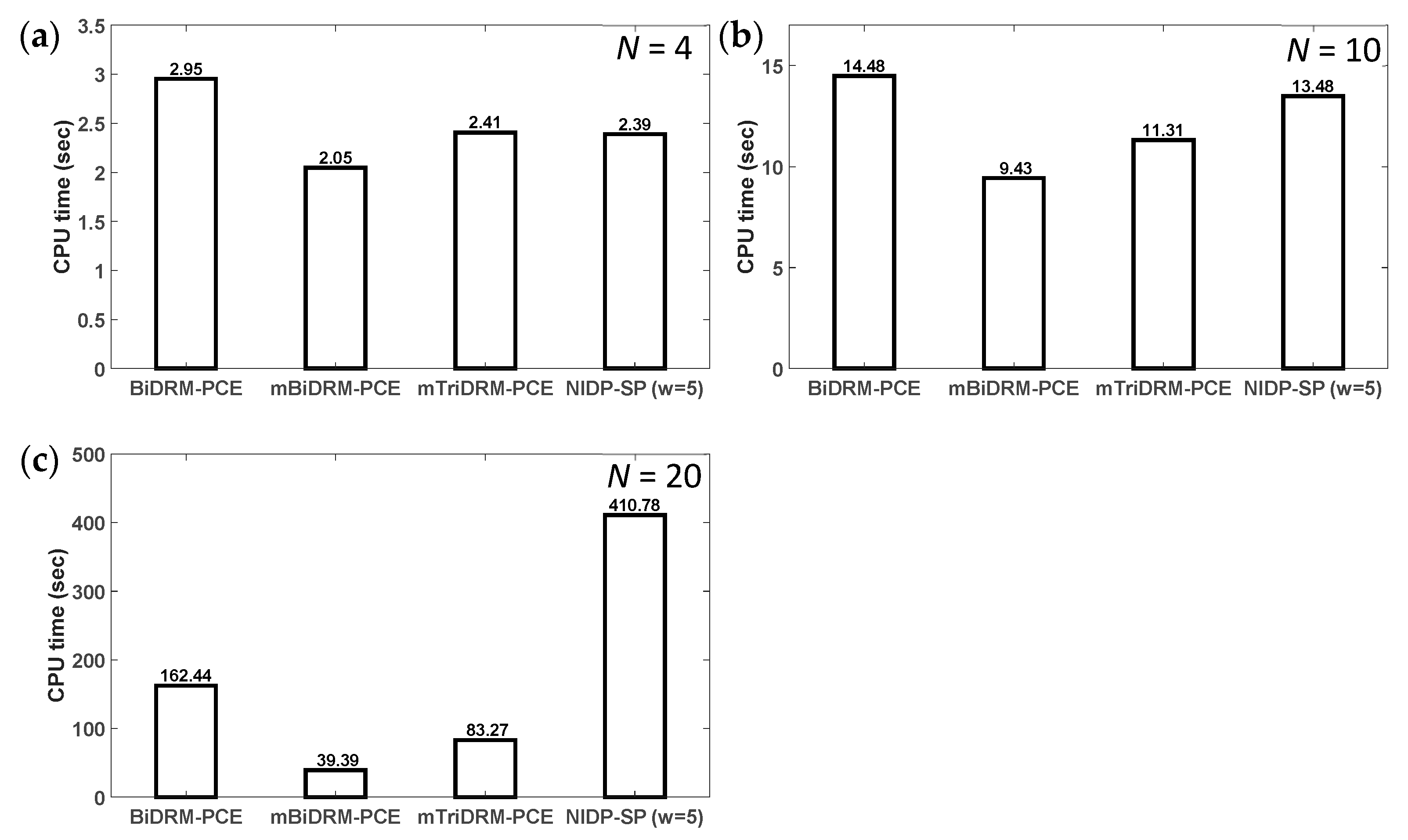
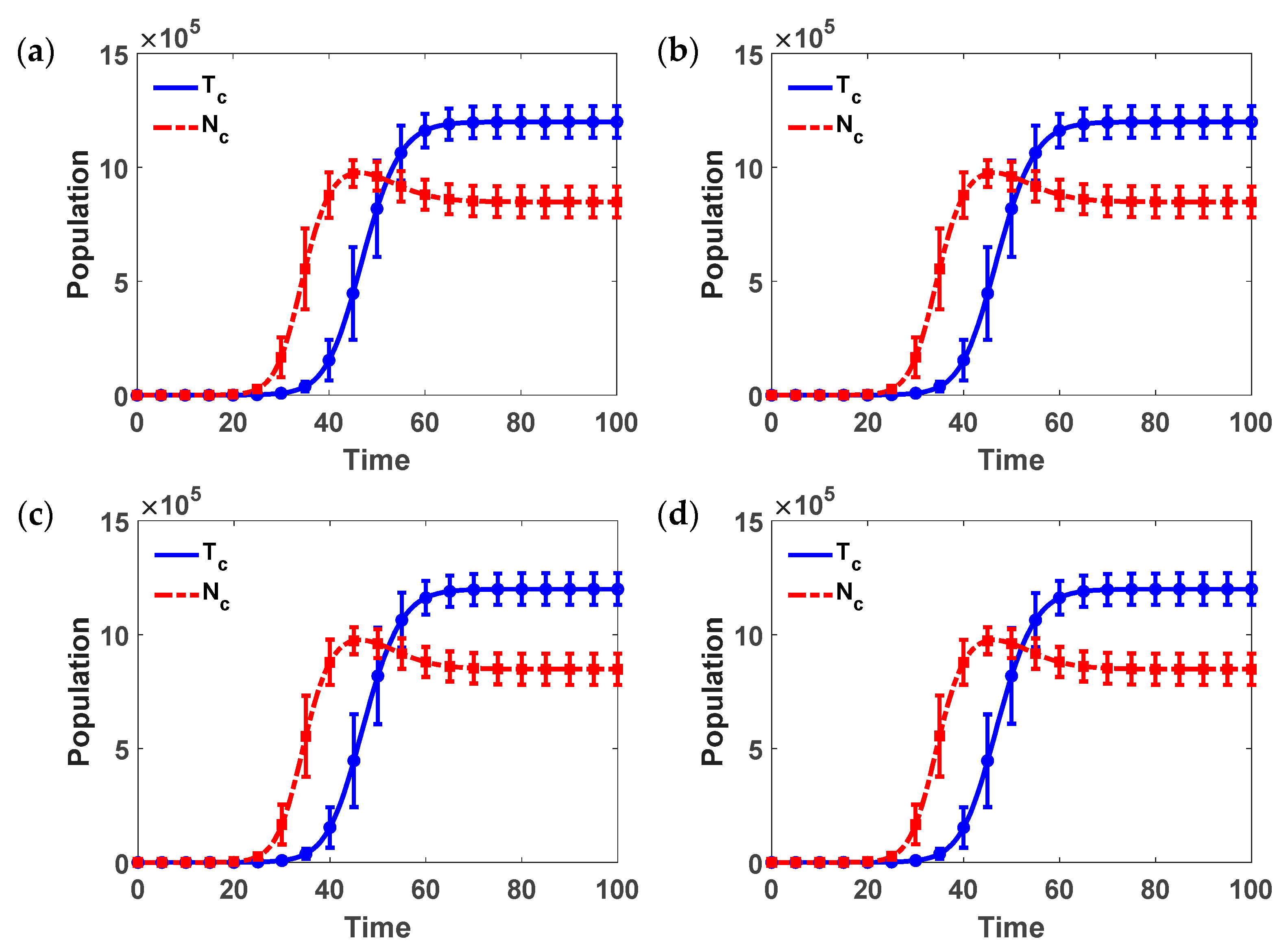
3.2. Example 2: Conjoint Tumor-Normal Cell Models

In this example, mathematical models [31], describing the mutual interactions between tumor and normal cells, were used to show the efficiency of the proposed UQ methods. This model was chosen since it is sufficiently complicated to show the capability of the UQ methods for dealing with many uncertainties. In addition, to obtain accurate model predictions, it is useful to consider intrinsic variability in tumor-environmental interactions. For example, a probabilistic description of model predictions, estimated with UQ techniques, can provide information to design multi-therapeutic strategies and to advance understanding of the growth of tumor cells. The model to describe cellular interactions can be described as follows [31]:
d T c d t = r T T c ( 1 T c K T ) β ( ρ 0 N c ρ 1 + N c )
d N c d t = r N N c ( 1 N c K N ) + κ T c ( 1 T c T * ) ,
where T c and N c denote the total number of tumor and normal cells, respectively. The description of these model parameters and their values used in this work are given in Table 1 [31]. All parameters in Equations (31) and (32) were assumed to be uncertain, that is, the number of uncertainties N is 9, generating a nine-dimensional random space. Also, all parametric uncertainties were assumed to be identically and uniformly distributed. Thus, Legendre polynomials were used here as the PCE basis functions. For clarity, the mathematical expression of each parametric uncertainty can be given as δ i = δ i ( 1 + σ ξ i ) , where δ i is the mean value of each parameter listed in Table 1 and ξ i is a random variable—uniformly distributed in the range of ( 1 , 1 ) . In this case study, we introduced 10% uncertainty into each parameter and subsequently, σ was set to 0.1. As done in Section 3.1, different UQ methods, including the mBiDRM-, mTriDRM-PCE methods and nonintrusive NIDP-SP, were used in this case study. The results with different UQ methods were shown in Figure 5. The approximation level w of NIDP-SP was set to 5. Note that the polynomial order of each uncertainty P is set to 2, which results in 55 PCE coefficients for each response, that is, 55 coupled ODEs are used to approximate each model prediction with the PCE theory (see Equation (5)). Since there are two model responses as described in Equations (31) and (32), a total of 110 equations are generated to describe the original stochastic system in this example. These coupled ODEs were numerically solved using the explicit second-order Runge-Kutta method [38]. For simulations, the initial value of the first coefficient of each model response (i.e., T c and N c ) was set to 1, while the rest of the coefficients were set to 0. Note that the equation corresponding to the first coefficient of the model response describes the mean value of its response in the presence of uncertainty.
Since 9 parametric uncertainties were considered, the BiDRM-PCE converted each nine-dimensional integral in the SG step into 36 two-dimensional and 9 one-dimensional integrals, while the TriDRM-PCE required to calculate 84 three-dimensional, 36 two-dimensional and 9 one-dimensional integrals. For mBiDRM- and mTriDRM-PCE methods, the Gauss-Legendre quadrature rules were used to generate 5 evaluation points in each dimension and the full tensor product was used to decide the total required evaluation points to estimate these low-dimensional integrals mentioned above. For the nonintrusive NIDP-SP, the Clenshaw-Curtis quadrature rules were used to generate sparse grids following the Smolyak algorithm, which contains 26,017 grid points, since N was set to 9. As seen in Figure 5, the mean values of T c and N c calculated with different UQ methods are shown with solid and dash-dot lines, respectively, while the error bars in each subplot show the uncertainty in model predictions at 21 discrete time points of the entire simulation (i.e., Time from 0 to 100 in Figure 5).
To compare the UQ accuracy, 105 samples for each parametric uncertainty were used for MC; and the simulation results were used as a reference in Equation (28). The RMSE of each method is given in Figure 6. Unlike the nonlinear algebraic problems in Section 3.1, simulation results of 21 discrete points over the entire simulation as shown in Figure 5 was used to calculate RMSE, that is, H = 21 in Equation (28). As seen in Figure 6, all methods show the identical RMSE results, indicating the accuracy of the methods in this work. We also compared the computational time as shown in Figure 7 to show the computational efficiency. As seen in Figure 7, compared to the NIDP-SP, the mBiDRM-PCE can reduce the computational time by about 43 percent points and the mTriDRM-PCE can save the computational time by approximately 33 percent points. This clearly shows that the superior performance of mBiDRM- and mTriDRM-PCE methods, when dealing with many uncertainties (up to 9 in this case study).

3.3. Example 3: G2 to Mitosis Transition Model for Fission Yeast

This example describes dynamic behaviors of living cells (fission yeast cells) in the transition phase from G2 to Mitosis (G2-M) in the cell cycle [32]. For simplicity, it is assumed that cells in the G2 phase, which have completed DNA replication, grow and prepare for mitosis—cells are divided into daughter cells. It is important to understand the transition mechanism, since it determines the time for mitotic entry and the cell size at the point of mitosis, at which cells divide into daughter cells. In addition, it provides useful information to investigate the impact of missense mutations in proteins on the genotype-phenotype relationship [32]. But model parameters cannot be well calibrated with data from biological experiments, due to the strong nonlinearity in model structure. Therefore, it can be useful to consider uncertainties in model parameters to improve the accuracy of model predictions. For fission yeast, the proteins, including cyclin-dependent kinase 1 (Cdk1), cyclin B (CycB), kinase Wee1 and phosphatase Cdc25, are involved in the G2 phase [32]. In this phase, a complex, that is, mitosis promoting factor (MPF) is formed by binding of Cdk1 to CycB, which leads to the G2-M transition. Details about the mechanism of this biological process can be found in the literature [32]. The model to describe the G2-M transition consists of the concentrations of CycB, MPF, Wee1 and Cdc25 (i.e., C C y c B , C M P F , C W e e 1 and C C d c 25 ), which are given as follows [32]:
d C C y c B d t = k s k d · C C y c B
d C M P F d t = V 25 · ( C C y c B C M P F ) V w e e · C M P F k d · C M P F
d C W e e 1 d t = k a w e e · ( 1 C W e e 1 ) J a w e e + 1 C W e e 1 k i w e e · C M P F · C W e e 1 J i w e e + C W e e 1
d C C d c 25 d t = k a 25 · C M P F · ( 1 C C d c 25 ) J a 25 + 1 C C d c 25 k i 25 · C C d c 25 J i 25 + C C d c 25
V 25 = k 25 · ( 1 C C d c 25 ) + k 25 · C C d c 25
V w e e = k w e e · ( 1 C W e e 1 ) + k w e e · C W e e 1 ,
where V 25 and V w e e are coefficients to determine the activation and inactivation rates of MPF. Model parameters and their corresponding descriptions are given in Table 2 [32]. Note that uncertainties in the concentration of CycB and MPF ( C C y c B and C M P F ), resulting from parametric uncertainties, are studied, since the MPF activity is controlled by Wee1 and Cdc25. It is also assumed in this work that all rate constants, excluding the Michalis constants, involve uncertainty in order to validate the performance of the presented UQ method. Thus, the resulting number of parametric uncertainties is 10 in this case study ( N = 10 ), which results in a ten-dimensional random space. In addition, as done in Section 3.2, the polynomial order of each uncertainty P is set to 2. Since there are ten uncertainties and P is 2, each of the model responses in Equations (33) to (36) consists of 66 ODEs, which results in 264 coupled ODEs to represent the original stochastic system. Similar to the previous example, 10% uncertainty was introduced into uncertain parameters; and it was assumed that each of them was randomly chosen from a uniform distribution in ( 1 , 1 ) . Thus, the rate constants, δ = ( k s , k d , k a w e e , k i w e e , k a 25 , , k i 25 , k 25 , k 25 , k w e e , k w e e ) in Equations (33) to (38) can be rewritten as δ i = δ i ( 1 + σ ξ i ) , where δ i is the mean value of each parameter, which can be found in Table 2. As done in the previous example, Legendre polynomials were used as PCE basis functions.
For brevity, in this case study, we focused on the comparison between the mTriDRM-PCE and the nonintrusive NIDP-SP methods. To quantify the UQ accuracy, MC simulations were also used to calculate the reference in Equation (28). For NIDP-SP, the approximation level w was set to 5. Based on the Smolyak algorithm, 41,265 collocation points were required, since the number of uncertainties N is 10. For MC, 105 samples were used for each parametric uncertainty. For the mTriDRM method, each 10-dimensional integral in the SG step was approximated with 120 three-dimensional, 45 two-dimensional and 10 one-dimensional integrals; and the full tensor product was used to construct evaluation points with 5 quadrature points of each uncertainty. Figure 8 shows the simulation results, where the explicit second-order Runge-Kutta method [38] was used to solve the differential equations formulated by the PCE theory. The initial conditions for the first coefficients of four model responses C C y c B , C M P F , C W e e 1 and C C d c 25 in Equations (33) to (36) were set to 0.01, 0.01, 1.0, 0.01, respectively, while the rest of the coefficients of each response were set to 0.
As seen in Figure 8, the solid and dash-dot lines show the mean values of C C y c B and C M P F , respectively, while error bars show the uncertainty of model predictions at 21 simulation time points. It is found that different UQ methods, mTriDRM-PCE, NIDP-SP and MC, provide similar UQ results. To quantify the UQ accuracy, the RMSEs of the mTriDRM-PCE and NIDP-SP methods were calculated and given in Table 3. Once again, the RMSE was computed with 21 discrete points in the 20 min simulation as shown in Figure 8 and H is 21 in Equation (28). We also compared the computational time of mTriDRM-PCE and NIDP-SP methods. As seen in Table 3, the simulation time of the NIDP-SP is almost doubled, as compared to the mTriDRM PCE. This clearly shows the advantage of the UQ method proposed in this work.

4. Conclusions

An efficient uncertainty quantification (UQ) method is developed by coupling the quadrature rules and the generalized dimension reduction method (gDRM) with the polynomial chaos expansion (PCE). To reduce the computational cost, especially when dealing with high-dimensional UQ problems, Gauss quadrature rules are used to numerically estimate low-dimensional integrals from the gDRM-based PCE. To show the efficiency of the method, the modified bivariate and trivariate dimension reduction based PCE (mBiDRM- and mTriDRM-PCE) are compared with different UQ methods, including the sparse grids-based nonintrusive discrete projection method (NIDP-SP), in terms of UQ accuracy and computational time. Our results show that the proposed UQ algorithm provides accurate UQ results and has superior performance (e.g., less computational time), as compared to other existing techniques (e.g., NIDP-SP). This lays the foundation to investigate more complicated problems in the future, which include the regulation and optimization of biological processes.

Author Contributions

Conceptualization, Y.D.; methodology, Y.D. and J.S.; validation, J.S.; investigation, J.S.; writing—original draft preparation, J.S.; writing—review and editing, Y.D., D.D.; supervision, Y.D. All authors have read and agreed to the published version of the manuscript.

Funding

This work was partially supported by the National Science Foundation, Division of Civil, Mechanical and Manufacturing Innovation (CMMI), under the award No. 1727487 and No. 1728338.

Conflicts of Interest

The authors declare no conflict of interest.

Abbreviations

BiDRMBivariate dimension reduction method
FTFull tensor grids method used for NIDP-based UQ
gDRMGeneralized dimension reduction method
GQGaussian quadrature
MCMonte Carlo
NIDPNonintrusive discrete projection
PCEPolynomial chaos expansion
PDFProbability density function
RMSERoot-mean-square error
SCStochastic collocation
SGStochastic Galerkin
SPSparse grids method used for NIDP-based UQ
TriDRMTrivariate dimension reduction method
UQUncertainty quantification

Appendix A

When the number of uncertainties is set to 4, Equation (29) of Example 1 in Section 3.1 is used to show the explicit expressions of the PCE coefficients. Following the procedure described in Section 2.1, when the polynomial order P = 2 , each parametric uncertainty X i ( i = 1 ,   2 ,   3 ,   4 ) and the model response Z 1 in Example 1 can be represented as:
X i = k = 0 P X ¯ i , k ψ k ( θ i ) = X ¯ i , 0 ψ 0 ( θ i ) + X ¯ i , 1 ψ 1 ( θ i ) + X ¯ i , 2 ψ 2 ( θ i )
Z 1 ( θ ) = m = 0 M Z ¯ 1 , m Ψ m ( θ ) = 0.5 + i = 1 N = 4 ( k = 0 P = 2 X ¯ i , k ψ k ( θ i ) ) 2 1 + 0.1 i = 1 N = 4 k = 0 P = 2 X ¯ i , k ψ k ( θ i )
where θ i is the i th random variable to describe the PDF of X i and { ψ k ( θ i ) } and Ψ m ( θ ) are the one-dimensional and four-dimensional Hermite polynomials. Following the procedures in Section 2.1, each PCE coefficient, that is, Z ¯ 1 , m can be formulated as:
Z ¯ 1 , m = 1 γ m N Z 1 ( θ ) Ψ m ( θ ) W ( θ ) d θ = 1 γ m N 0.5 + i = 1 N = 4 ( k = 0 P = 2 X ¯ i , k ψ k ( θ i ) ) 2 1 + 0.1 i = 1 N = 4 k = 0 P = 2 X ¯ i , k ψ k ( θ i ) Ψ m ( θ ) W ( θ ) d θ
where γ m = E [ Ψ m 2 ] and W ( θ ) is a weight function determined by the joint PDF of θ . The calculation of four-dimensional integral in Equation (A3) can be done in a computationally efficient manner by using gDRM technique. Here we present an example when BiDRM is used to evaluate the integral in Equation (A3) but other gDRM such as TriDRM can be used, depending on the dimension of the integral.
By converting the four-dimensional integral into low-dimensional ones using the BiDRM, which only involve at most two variables, the coefficient Z ¯ 1 , m can be redefined as:
Z ¯ 1 , m 1 γ m [ ω 1 < ω 2 { y ( θ ω 1 , θ ω 2 , 0 ω 1 ω 2 ) W ( θ ¯ ) d θ ¯ } 2 × ω 1 { y ( θ ω 1 , 0 ω 1 ) W ( θ ω 1 ) d θ ω 1 } + 3 × y ( 0 ) ]
where y ( θ ) = Z 1 ( θ ) Ψ m ( θ ) . In addition, 0 ω 1 ω 2 represents the zero vector excluding the ω 1 th and ω 2 th elements. Similarly, the element ω 1 th is excluded in the zero vector 0 ω 1 [39]. The proposed approach calculates each integral in Equation (A4) with the quadrature rules as:
Z ¯ 1 , m 1 γ m [ ω 1 < ω 2 { q 1 = 1 Q 1 q 2 = 1 Q 2 y ( θ ω 1 q 1 , θ ω 2 q 2 , 0 ω 1 ω 2 ) · ( α ω 1 q 1 α ω 2 q 2 ) } 2 × ω 1 { q 1 = 1 Q 1 y ( θ ω 1 q 1 , 0 ω 1 ) · α ω 1 q 1 } + 3 × y ( 0 ) ]
For example, when ω 1 and ω 2 are set to 1 and 2, respectively, the function y in the summation to evaluate the two-dimensional integrals can be given as:
y ( θ 1 q 1 , θ 2 q 2 , 0 12 ) = Z 1 ( θ 1 q 1 , θ 2 q 2 , 0 12 ) Ψ m ( θ 1 q 1 , θ 2 q 2 , 0 12 ) Z 1 ( θ 1 q 1 , θ 2 q 2 , 0 12 ) = 0.5 + ( k = 0 P = 2 X ¯ 1 , k ψ k ( θ 1 q 1 ) ) 2 + ( k = 0 P = 2 X ¯ 2 , k ψ k ( θ 2 q 2 ) ) 2 + ( X ¯ 3 , 0 X ¯ 3 , 2 ) 2 + ( X ¯ 4 , 0 X ¯ 4 , 2 ) 2 1 + 0.1 ( k = 0 P = 2 X ¯ 1 , k ψ k ( θ 1 q 1 ) + k = 0 P = 2 X ¯ 2 , k ψ k ( θ 2 q 2 ) + ( X ¯ 3 , 0 X ¯ 3 , 2 ) + ( X ¯ 4 , 0 X ¯ 4 , 2 ) )
Similarly, the function y of the first term in the summation to calculate one-dimensional integrals (i.e., ω 1 = 1 ) can be defined as follows:
y ( θ 1 q 1 , 0 1 ) = Z 1 ( θ 1 q 1 , 0 1 ) Ψ m ( θ 1 q 1 , 0 1 ) Z 1 ( θ 1 q 1 , 0 1 ) = 0.5 + ( k = 0 P = 2 X ¯ 1 , k ψ k ( θ 1 q 1 ) ) 2 + ( X ¯ 2 , 0 X ¯ 2 , 2 ) 2 + ( X ¯ 3 , 0 X ¯ 3 , 2 ) 2 + ( X ¯ 4 , 0 X ¯ 4 , 2 ) 2 1 + 0.1 ( k = 0 P = 2 X ¯ 1 , k ψ k ( θ 1 q 1 ) + ( X ¯ 2 , 0 X ¯ 2 , 2 ) + ( X ¯ 3 , 0 X ¯ 3 , 2 ) + ( X ¯ 4 , 0 X ¯ 4 , 2 ) )
For the last term in Equation (A5), the function y ( 0 ) can be expressed as:
y ( 0 ) = Z 1 ( 0 ) Ψ m ( 0 ) Z 1 ( 0 ) = 0.5 + ( X ¯ 1 , 0 X ¯ 1 , 2 ) 2 + ( X ¯ 2 , 0 X ¯ 2 , 2 ) 2 + ( X ¯ 3 , 0 X ¯ 3 , 2 ) 2 + ( X ¯ 4 , 0 X ¯ 4 , 2 ) 2 1 + 0.1 ( ( X ¯ 1 , 0 X ¯ 1 , 2 ) + ( X ¯ 2 , 0 X ¯ 2 , 2 ) + ( X ¯ 3 , 0 X ¯ 3 , 2 ) + ( X ¯ 4 , 0 X ¯ 4 , 2 ) )
Note that Equation (A5) is the final expression to calculate the PCE coefficients for the mBiDRM-PCE based approach.

Appendix B

To compare the proposed algorithm with the classical PCE methods that rely on the intrusive spectral projection [16], the simulation results of Example 1 in Section 3.1 are shown in Figure A1. Of note, the PCE coefficients of Equation (29), involving nonlinear forms such as division and square root, were solved following the procedure in Reference [16] (see Sections 4.5.2 and 4.5.3 in Reference [16]). To derive the PCE coefficients of the square root, a nonlinear system solver ‘fsolve’ in MATLAB R2019a (MathWorks, Natick, MA, USA) is used. For Equation (30), the stochastic expansion of the logarithm term is determined based on the Taylor series approach [16,17] (see Section 2.3 in Reference [17]) and the number of terms in the Taylor series is set to 3 in this work. In addition, for the classical PCE method, the number of polynomial terms in the PCE expansion for the model responses in Equations (29) and (30) is 15 (i.e., M + 1 = 15 ) , considering that the number of uncertainties N is 4 and the polynomial order of each uncertainty P is 2.
Figure A1. Root-mean-square error (RMSE) of the model responses Z 1 and Z 2 with different UQ methods for comparison with the classical PCE method: the errors of the standard deviation of Z 1 and Z 2 are shown in (a,b), respectively.
Applmech 01 00011 g0a1
Compared to the classical PCE approaches, the UQ results obtained with the algorithm in this work have smaller RMSE errors in Figure A1, when the variability of uncertain parameters (i.e., σ ) increases. This shows the accuracy of the algorithm in this work, indicating its applicability to deal with more complex and nonlinear problems.

References

  1. Champagne, C.; Cazelles, B. Comparison of stochastic and deterministic frameworks in dengue modelling. Math. Biosci. 2019, 310, 1–12. [Google Scholar] [CrossRef] [PubMed]
  2. Harman, D.B.; Johnston, P.R. Applying the stochastic Galerkin method to epidemic models with uncertainty in the parameters. Math. Biosci. 2016, 277, 25–37. [Google Scholar] [CrossRef] [PubMed]
  3. Sullivan, T.J. Introduction to Uncertainty Quantification; Springer: Berlin, Germany, 2015. [Google Scholar]
  4. Marquis, A.D.; Arnold, A.; Dean-Bernhoft, C.; Carlson, B.E.; Olufsen, M.S. Practical identifiability and uncertainty quantification of a pulsatile cardiovascular model. Math. Biosci. 2018, 304, 9–24. [Google Scholar] [CrossRef] [PubMed] [Green Version]
  5. Vanlier, J.; Tiemann, C.; Hilbers, P.; Van Riel, N.A.W. Parameter uncertainty in biochemical models described by ordinary differential equations. Math. Biosci. 2013, 246, 305–314. [Google Scholar] [CrossRef]
  6. Gel, A.; Garg, R.; Tong, C.; Shahnam, M.; Guenther, C. Applying uncertainty quantification to multiphase flow computational fluid dynamics. Powder Technol. 2013, 242, 27–39. [Google Scholar] [CrossRef]
  7. Ma, D.L.; Braatz, R.D. Robust identification and control of batch processes. Comput. Chem. Eng. 2003, 27, 1175–1184. [Google Scholar] [CrossRef]
  8. Schenkendorf, R.; Xie, X.; Krewer, U. An efficient polynomial chaos expansion strategy for active fault identification of chemical processes. Comput. Chem. Eng. 2019, 122, 228–237. [Google Scholar] [CrossRef]
  9. Fishman, G.S. Monte Carlo: Concepts, Algorithms, and Applications; Springer: New York, NY, USA, 1996. [Google Scholar]
  10. Xiu, D. Numerical Methods for Stochastic Computations: A Spectral Method Approach; Princeton University Press: Princeton, NJ, USA, 2010. [Google Scholar]
  11. Wiener, N. The Homogeneous Chaos. Am. J. Math. 1938, 60, 897. [Google Scholar] [CrossRef]
  12. Streif, S.; Kim, K.-K.K.; Rumschinski, P.; Kishida, M.; Shen, D.E.; Findeisen, R.; Braatz, R.D. Robustness analysis, prediction, and estimation for uncertain biochemical networks: An overview. J. Process. Control. 2016, 42, 14–34. [Google Scholar] [CrossRef]
  13. Debusschere, B.J.; Najm, H.; Matta, A.; Knio, O.M.; Ghanem, R.; Le Maître, O.P. Protein labeling reactions in electrochemical microchannel flow: Numerical simulation and uncertainty propagation. Phys. Fluids 2003, 15, 2238. [Google Scholar] [CrossRef] [Green Version]
  14. Du, Y.; Budman, H.; Duever, T. Parameter Estimation for an Inverse Nonlinear Stochastic Problem: Reactivity Ratio Studies in Copolymerization. Macromol. Theory Simul. 2017, 26, 1600095. [Google Scholar] [CrossRef]
  15. Najm, H.N. Uncertainty Quantification and Polynomial Chaos Techniques in Computational Fluid Dynamics. Annu. Rev. Fluid Mech. 2009, 41, 35–52. [Google Scholar] [CrossRef]
  16. Le Maître, O.P.; Knio, O.M.; Le Maître, O. Spectral Methods for Uncertainty Quantification: With Applications to Computational Fluid Dynamics; Springer Science & Business Media: Berlin, Germany, 2010. [Google Scholar]
  17. Debusschere, B.J.; Najm, H.N.; Pébay, P.P.; Knio, O.M.; Ghanem, R.; Le Maître, O.P. Numerical Challenges in the Use of Polynomial Chaos Representations for Stochastic Processes. SIAM J. Sci. Comput. 2004, 26, 698–719. [Google Scholar] [CrossRef]
  18. Xiu, D.; Karniadakis, G.E. Modeling uncertainty in steady state diffusion problems via generalized polynomial chaos. Comput. Methods Appl. Mech. Eng. 2002, 191, 4927–4948. [Google Scholar] [CrossRef]
  19. Babuška, I.; Tempone, R.; Zouraris, G.E. Galerkin Finite Element Approximations of Stochastic Elliptic Partial Differential Equations. SIAM J. Numer. Anal. 2004, 42, 800–825. [Google Scholar] [CrossRef]
  20. Son, J.; Du, Y. Probabilistic surrogate models for uncertainty analysis: Dimension reduction-based polynomial chaos expansion. Int. J. Numer. Methods Eng. 2019, 121, 1198–1217. [Google Scholar] [CrossRef]
  21. Son, J.; Du, Y. Comparison of intrusive and nonintrusive polynomial chaos expansion-based approaches for high dimensional parametric uncertainty quantification and propagation. Comput. Chem. Eng. 2020, 134, 106685. [Google Scholar] [CrossRef]
  22. Xu, H.; Rahman, S. A generalized dimension-reduction method for multidimensional integration in stochastic mechanics. Int. J. Numer. Methods Eng. 2004, 61, 1992–2019. [Google Scholar] [CrossRef] [Green Version]
  23. McClarren, R.G. Gauss Quadrature and Multi-dimensional Integrals. In Computational Nuclear Engineering and Radiological Science Using Python; McClarren, R.G., Ed.; Academic Press: Cambridge, MA, USA, 2018; pp. 287–299. [Google Scholar]
  24. Cao, Y.; Chen, Z.; Gunzburger, M. ANOVA expansions and efficient sampling methods for parameter dependent nonlinear PDEs. Int. J. Numer. Anal. Mod. 2009, 6, 256–273. [Google Scholar]
  25. Eldred, M.; Burkardt, J. Comparison of Non-Intrusive Polynomial Chaos and Stochastic Collocation Methods for Uncertainty Quantification. In Proceedings of the 47th AIAA Aerospace Sciences Meeting including The New Horizons Forum and Aerospace Exposition, Orlando, FL, USA, 5–8 January 2009. [Google Scholar]
  26. Smolyak, S.A. Quadrature and interpolation formulas for tensor products of certain classes of functions. Sov. Math. Dokl. 1963, 4, 240–243. [Google Scholar]
  27. Judd, K.L.; Maliar, L.; Maliar, S.; Valero, R. Smolyak method for solving dynamic economic models: Lagrange interpolation, anisotropic grid and adaptive domain. J. Econ. Dyn. Control. 2014, 44, 92–123. [Google Scholar] [CrossRef] [Green Version]
  28. Xiu, D. Efficient collocational approach for parametric uncertainty analysis. Commun. Comput. Phys. 2007, 2, 293–309. [Google Scholar]
  29. Ganapathysubramanian, B.; Zabaras, N. Sparse grid collocation schemes for stochastic natural convection problems. J. Comput. Phys. 2007, 225, 652–685. [Google Scholar] [CrossRef]
  30. Kim, K.; Kim, J.; Kim, C.; Lee, Y.; Lee, W.B. Robust Design of Multicomponent Working Fluid for Organic Rankine Cycle. Ind. Eng. Chem. Res. 2019, 58, 4154–4167. [Google Scholar] [CrossRef]
  31. Feizabadi, M.S. Modeling the Effects of a Simple Immune System and Immunodeficiency on the Dynamics of Conjointly Growing Tumor and Normal Cells. Int. J. Boil. Sci. 2011, 7, 700–707. [Google Scholar] [CrossRef]
  32. Cheng, T.M.K.; Goehring, L.; Jeffery, L.; Lu, Y.-E.; Hayles, J.; Novak, B.; A Bates, P. A Structural Systems Biology Approach for Quantifying the Systemic Consequences of Missense Mutations in Proteins. PLoS Comput. Boil. 2012, 8, e1002738. [Google Scholar] [CrossRef] [Green Version]
  33. Xiu, D.; Karniadakis, G.E. The Wiener--Askey Polynomial Chaos for Stochastic Differential Equations. SIAM J. Sci. Comput. 2002, 24, 619–644. [Google Scholar] [CrossRef]
  34. Reagan, M.T.; Najm, H.N.; Ghanem, R.; Knio, O.M. Uncertainty quantification in reacting-flow simulations through non-intrusive spectral projection. Combust. Flame 2003, 132, 545–555. [Google Scholar] [CrossRef]
  35. Venkateshan, S.; Swaminathan, P. Computational Methods in Engineering; Elsevier: Amsterdam, The Netherlands, 2014. [Google Scholar]
  36. Jao, C. Efficient Decision Support Systems: Practice and Challenges from Current to Future; IntechOpen: London, UK, 2011. [Google Scholar]
  37. Hill, J.M.; Moore, R. Applied Mathematics Entering the 21st Century: Invited Talks from the ICIAM 2003 Congress; Society for Industrial and Applied Mathematics: Philadelphia, PA, USA, 2004. [Google Scholar]
  38. Griffiths, D.F.; Higham, D.J. Numerical Methods for Ordinary Differential Equations; Springer Science and Business Media: Berlin, Germany, 2010. [Google Scholar]
  39. Xu, J.; Dang, C. A new bivariate dimension reduction method for efficient structural reliability analysis. Mech. Syst. Signal Process. 2019, 115, 281–300. [Google Scholar] [CrossRef]
Figure 1. Schematic illustration of the modified the generalized dimension reduction method (gDRM)–polynomial chaos expansion (PCE) approach for uncertainty quantification (UQ).
Applmech 01 00011 g001
Figure 2. Root-mean-square error (RMSE) of the system responses Z 1 and Z 2 with different UQ methods: the errors of the mean and standard deviation of Z 1 are shown in (a,b), while the simulation results of Z 2 are given in (c,d). For each subplot, bivariate DRM (BiDRM-) and trivariate DRM (TriDRM)–PCE refer to the bivariate and trivariate dimension reduction based PCE, respectively. The modified algorithms, coupling the dimension reduction with quadrature rules, are termed as modified BiDRM (mBiDRM-) and modified TriDRM (mTriDRM)-PCE, respectively. The nonintrusive discrete projection (NIDP) represents the nonintrusive UQ methods in PCE theory and FT and SP refer to full-tensor grids and sparse grids of collocation points, respectively. The Trapezoid-PCE represents that the trapezoidal rules were used to solve the high-dimensional integrals in the stochastic Galerkin (SG) projection.
Applmech 01 00011 g002
Figure 3. RMSE of the resulting statistics evaluated with different UQ methods in N = 4, 10 and 20: RMSEs of mean and standard deviation for Z 1 are shown in (a,b) and for Z 2 are given in (c,d), respectively.
Applmech 01 00011 g003
Figure 4. Comparison of computational time of different methods with different numbers of uncertainties: (a) N = 4, (b) N = 10 and (c) N = 20.
Applmech 01 00011 g004
Figure 5. Comparison of the UQ results of the cell populations T c and N c with different methods: (a) mBiDRM-PCE, (b) mTriDRM-PCE, (c) NIDP-SP with w = 5 and (d) MC simulations. The unit of time is not given here because it is problem-specific as noted in Reference [31].
Applmech 01 00011 g005
Figure 6. RMSE of the resulting statistics in the cell populations T c and N c calculated with different UQ methods: (a) the RMSE of mean value and (b) the RMSE of standard deviation.
Applmech 01 00011 g006
Figure 7. Comparison of computational time of different methods with the tumor-normal cell models.
Applmech 01 00011 g007
Figure 8. Comparison of UQ results of C C y c B and C M P F with different methods: (a) mTriDRM-PCE, (b) NIDP-SP with w = 5 and (c) MC simulations.
Applmech 01 00011 g008
Table 1. Parameters and their description in the tumor-normal cell interaction models [31].
ParametersDescription of Model ParametersValuesUnits
r T The growth rate for the tumor cells0.3Time−1
K T Carrying capacity of tumor cells 1.2 × 10 6 Cells
r N The growth rate for the normal cells0.4Time−1
K N Carrying capacity of normal cells 1.0 × 10 6 Cells
β Normal-tumor cell interaction rate1Time−1
ρ 0 Interaction clearance term1Cells
ρ 1 Half-saturation for interaction1000Cells
κ Tumor-normal cell interaction rate0.014Time−1
T * Critical size of the tumor 3.0 × 10 5 Cells
Table 2. Parameters and their description in the G2-M transition model [32].
ParametersDescription of Model ParametersValuesUnits
k s Rate constant of CycB synthesis0.2min−1
k d Degradation rates of CycB and MPF0.008min−1
k a w e e Rate constant of Wee1 being activated by a phosphatase0.61min−1
k i w e e Rate constant of Wee1 being inactivated by MPF0.71min−1
k a 25 Rate of Cdc25 being activated by MPF0.80min−1
k i 25 Rate of Cdc25 being inactivated by a phosphatase0.35min−1
k 25 Turnover coefficient for the activation rate of MPF, V 25 0.008min−1
k 25 Turnover coefficient for the activation rate of MPF, V 25 0.89min−1
k w e e Turnover coefficient for the inactivation rate of MPF, V w e e 0.03min−1
k w e e Turnover coefficient for the inactivation rate of MPF, V w e e 0.18min−1
J a w e e Michaelis constant of MPF for Cdc250.90-
J i w e e Michaelis constant of MPF for Wee10.21-
J a 25 Michaelis constant of phosphatase for Cdc250.19-
J i 25 Michaelis constant of phosphatase for Wee10.93-
Table 3. Comparison of different approaches in terms of UQ accuracy and computational time.
UQ MethodsRSMEMEANRSMESTDCPU Time (Hour)
C C y c B C M P F C C y c B C M P F
mTriDRM-PCE0.0001550.0002172.04 × 10−53.80 × 10−57.30
NIDP-SP (w = 5)0.0002780.0003383.37 × 10−50.00021811.86

