Damage Evaluation of Free-Free Beam Based on Vibration Testing

 ,
, 
Abstract
1. Introduction
2. Steel Beam Experiments
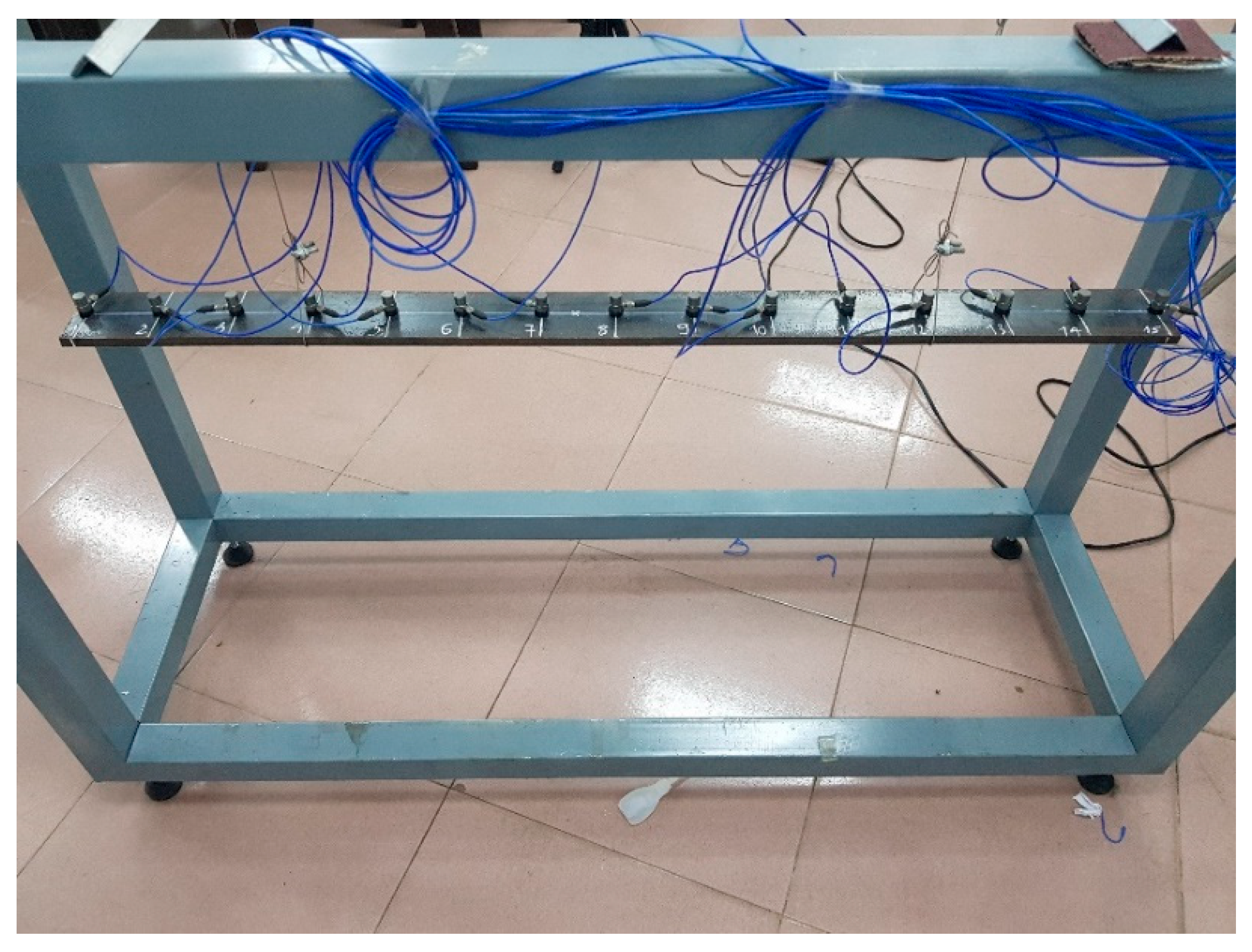
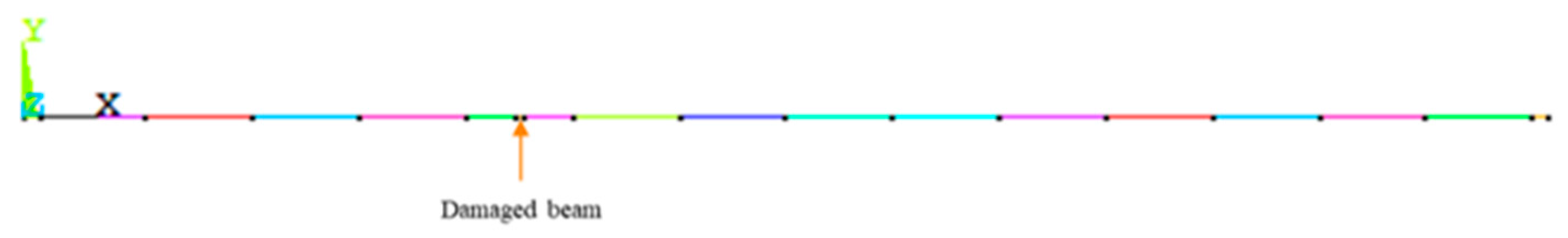
2.1. Experimental Setup
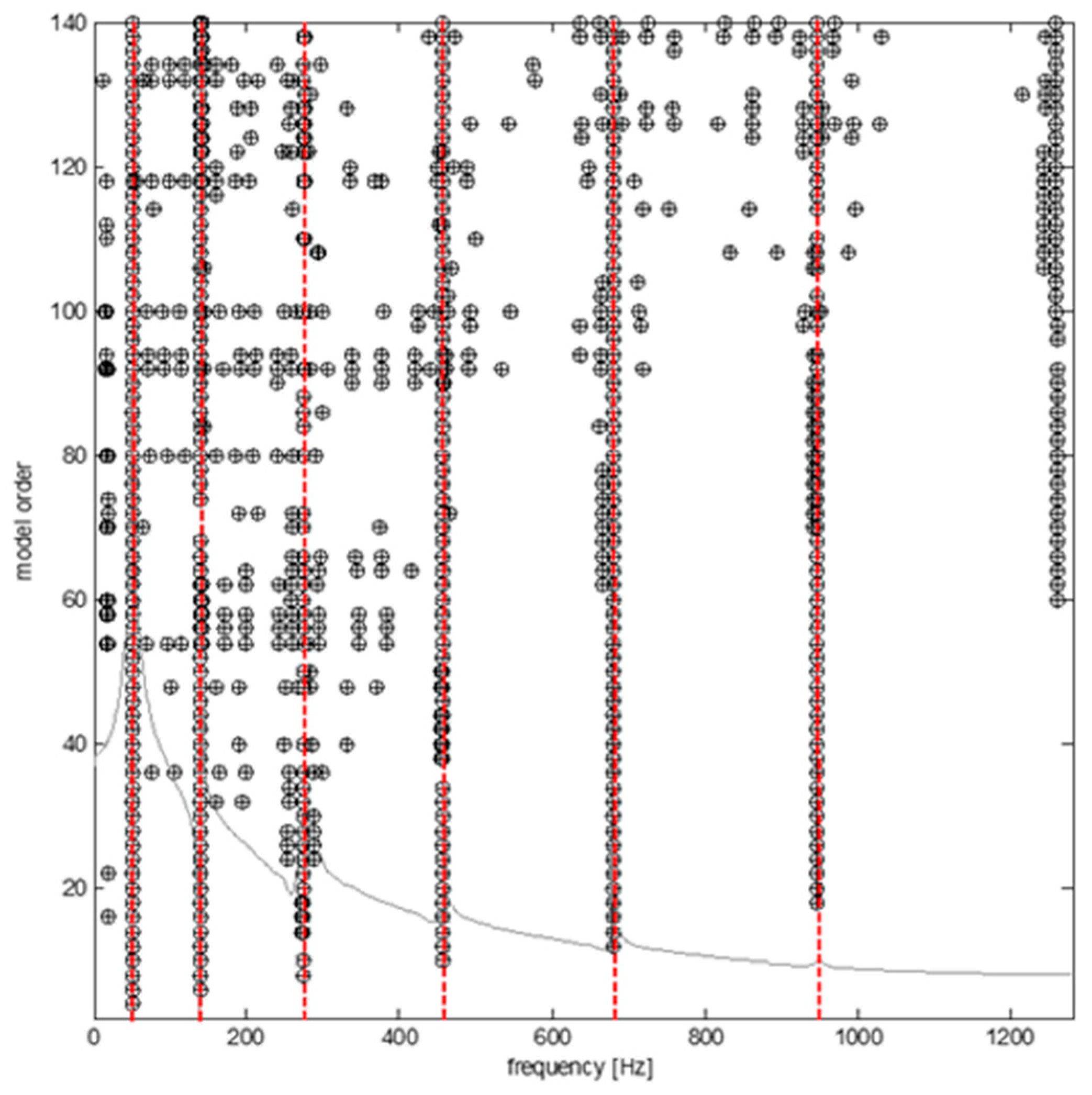
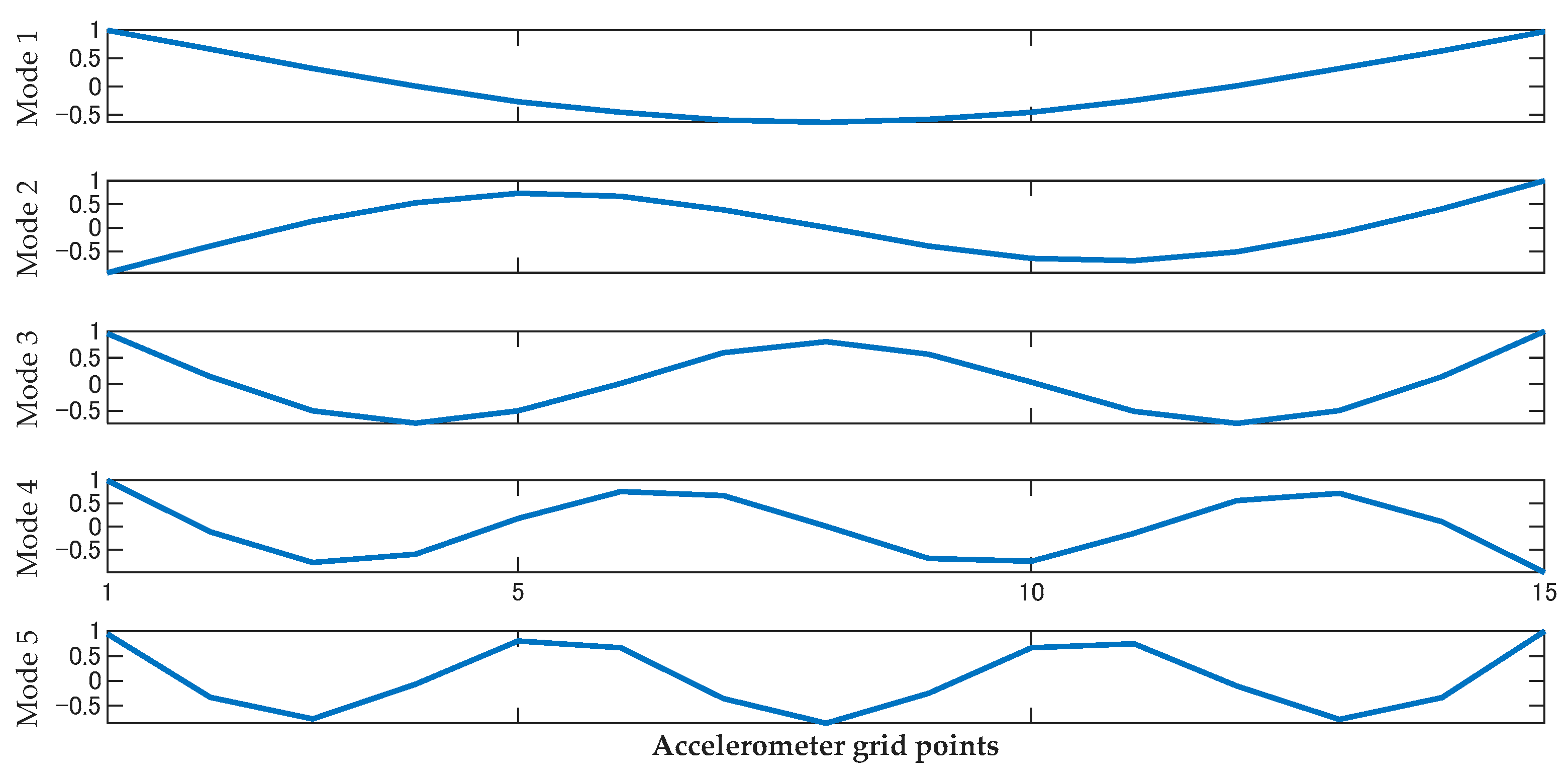
2.2. Experimental Results
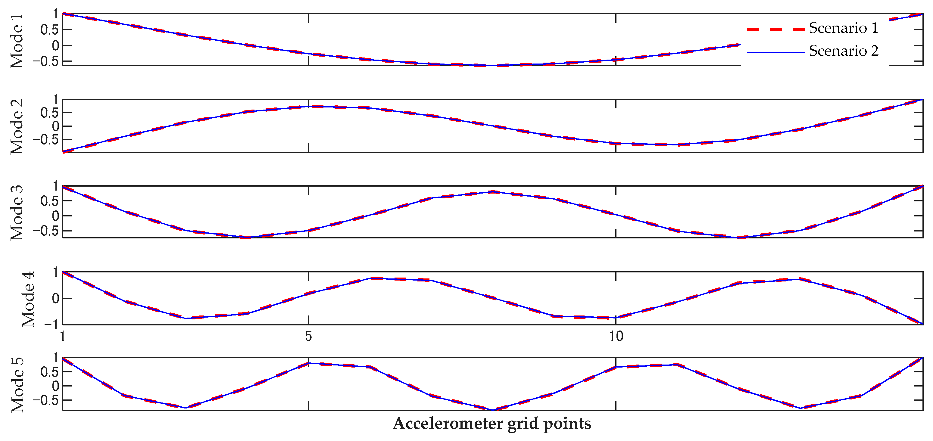
2.2.1. Intact Beam
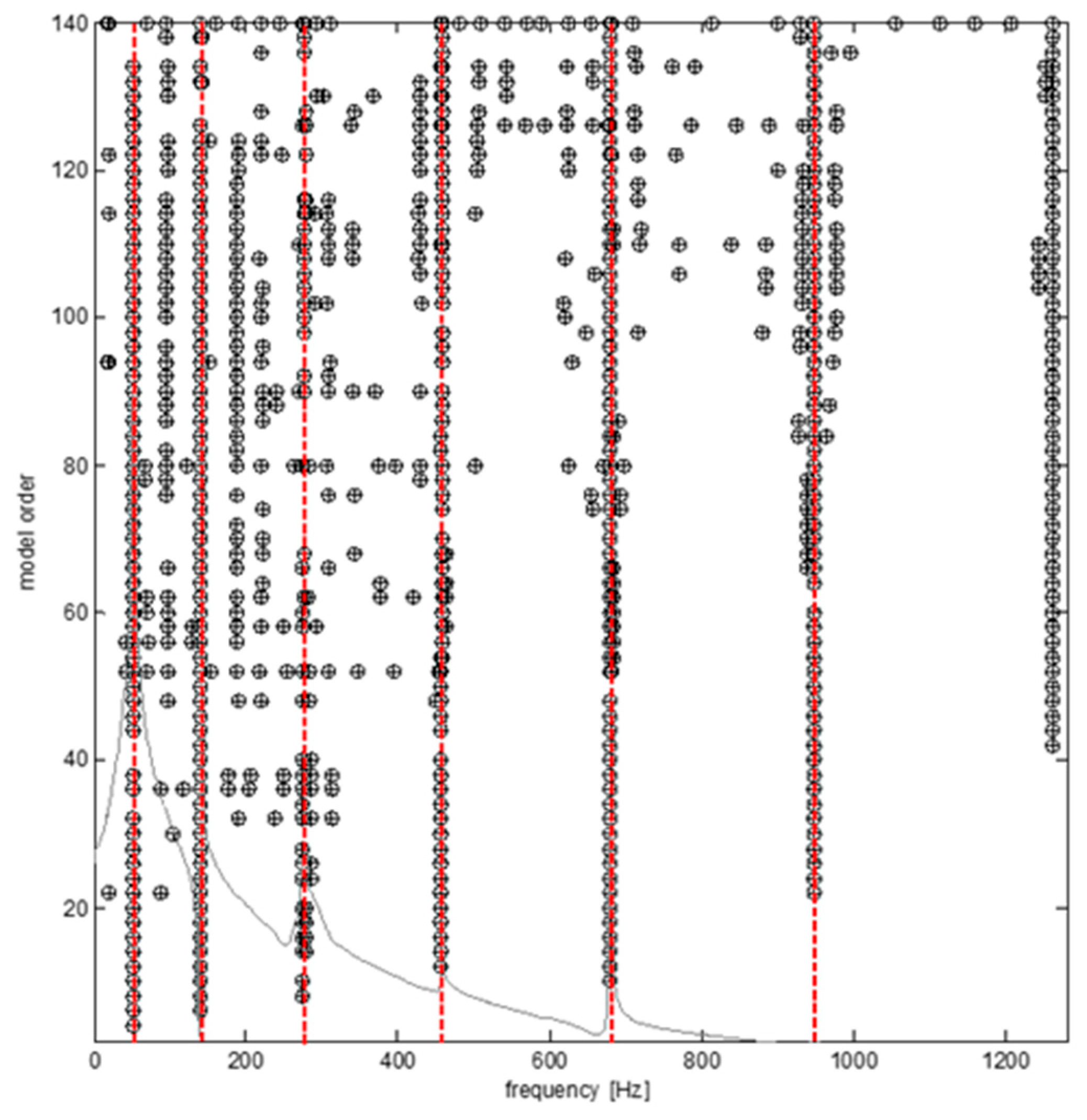
2.2.2. Damaged Beam
3. Numerical Models
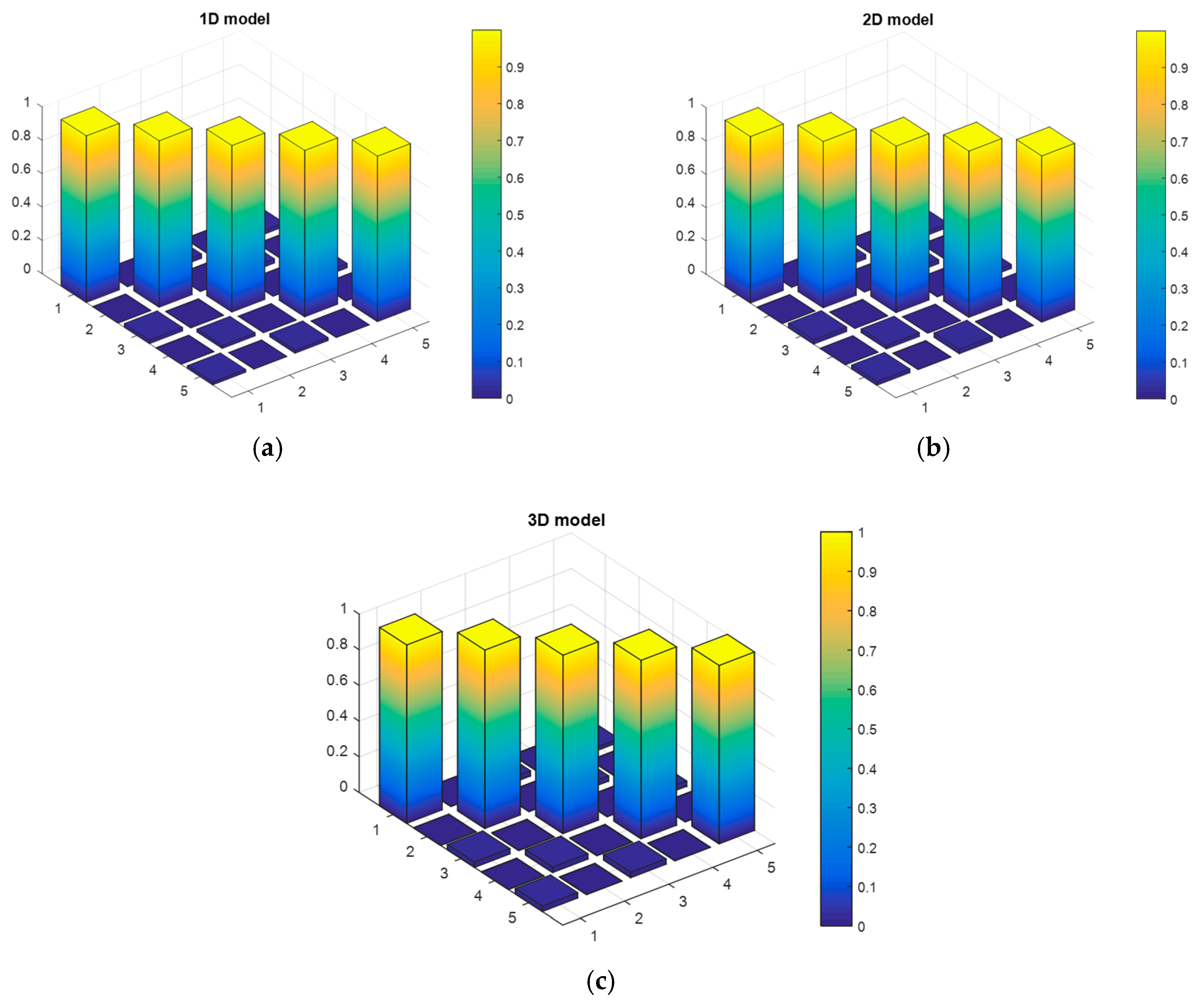
3.1. Beam Model (1D Model)
3.2. Shell Model (2D Model)
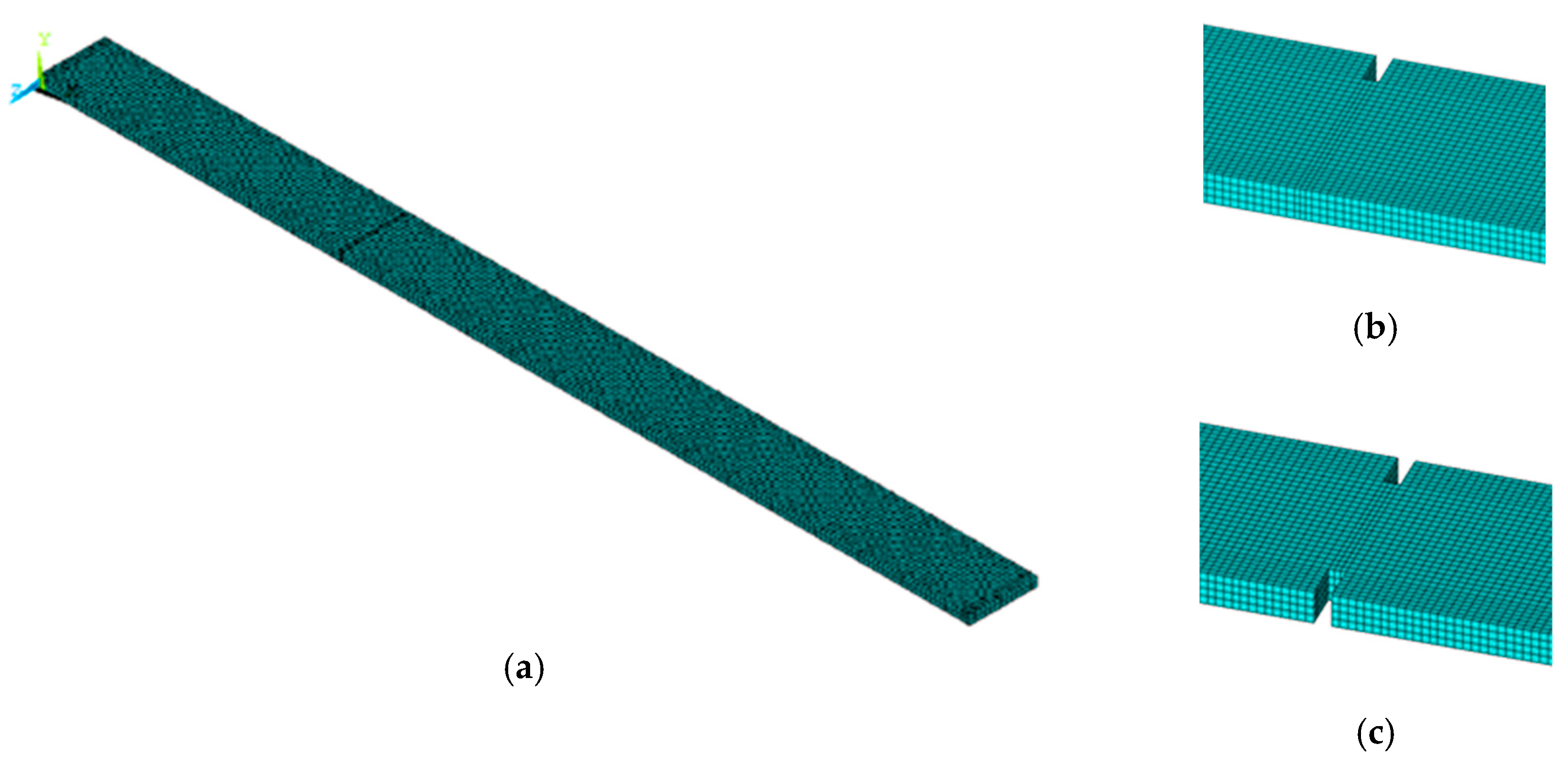
3.3. Solid Model (3D Model)
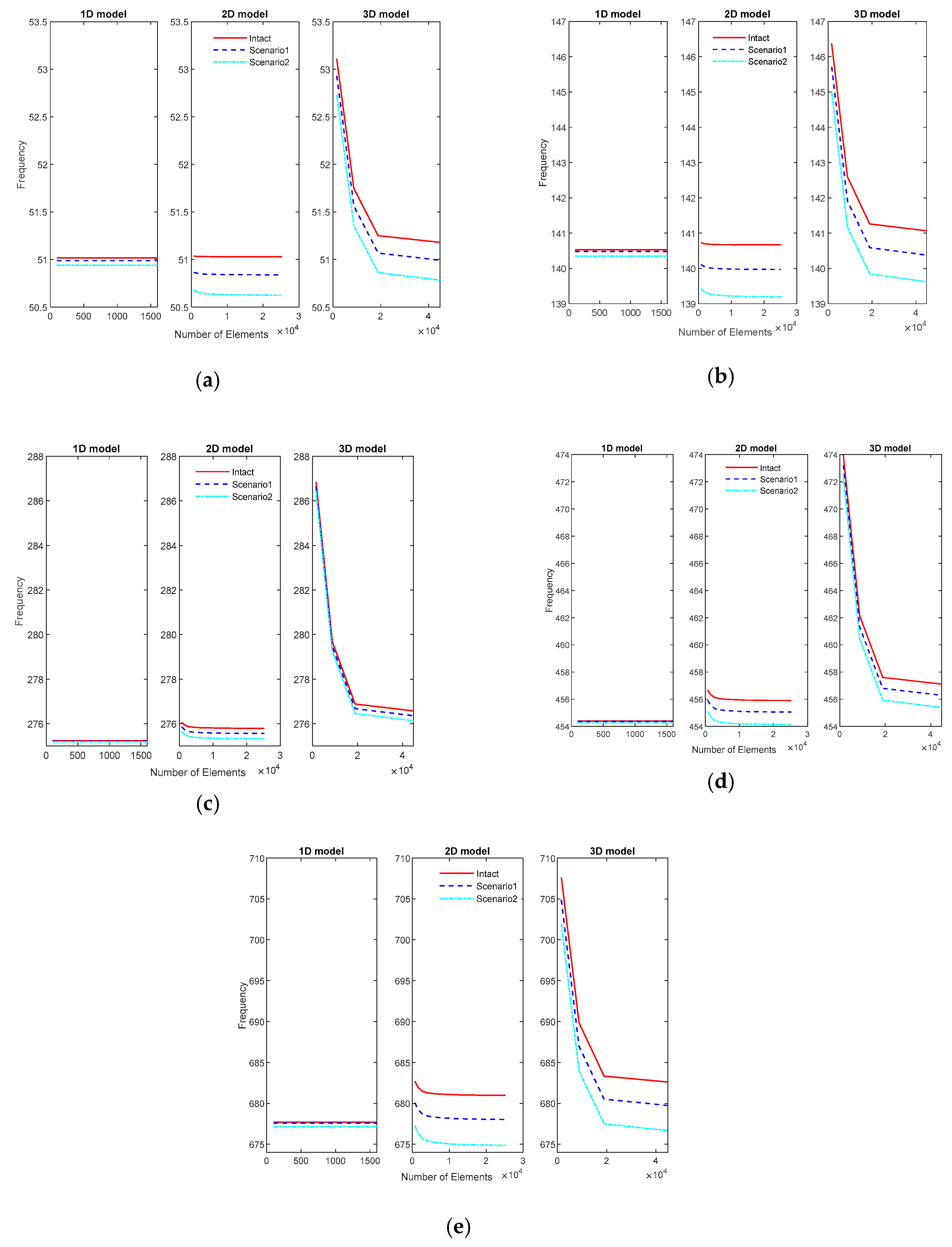
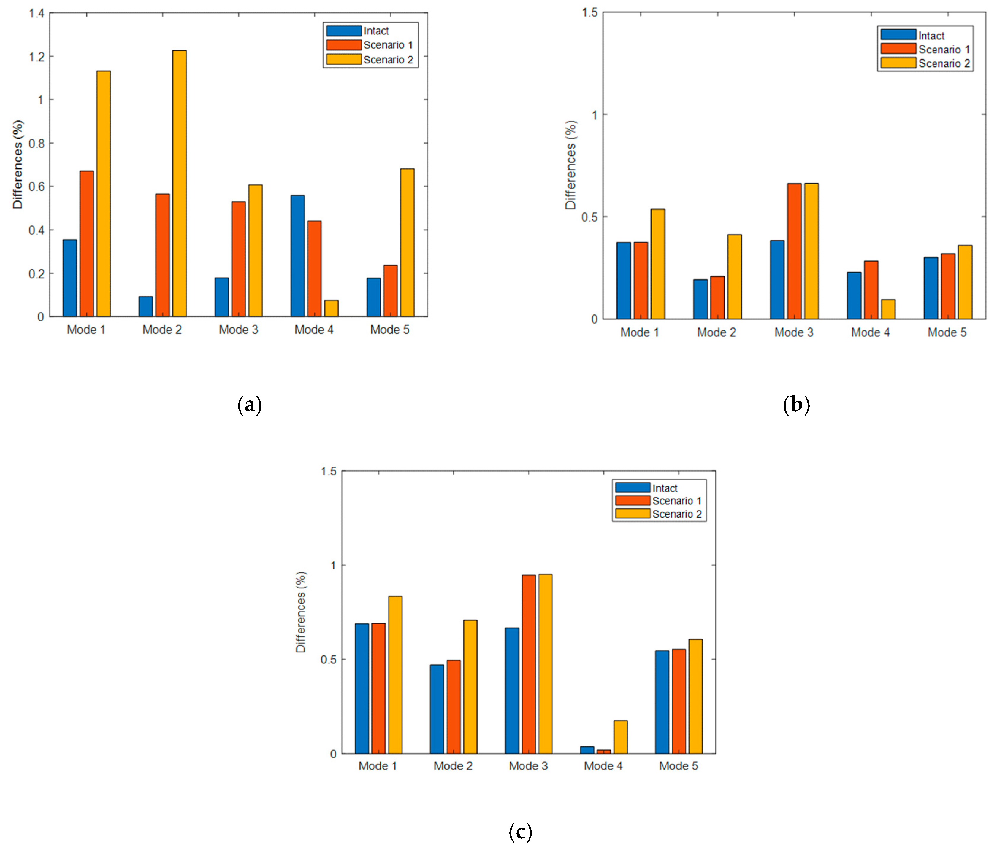
4. Results and Discussion
5. Conclusions
Author Contributions
Funding
Conflicts of Interest
References
- Carden, E.P.; Fanning, P. Vibration based condition monitoring: A review. Struct. Health Monit. 2004, 3, 355–377. [Google Scholar] [CrossRef]
- Maia, N.; Silva, J.; Almas, E.; Sampaio, R. Damage detection in structures: From mode shape to frequency response function methods. Mech. Syst. Signal Process. 2003, 17, 489–498. [Google Scholar] [CrossRef]
- Yan, Y.; Cheng, L.; Wu, Z.; Yam, L. Development in vibration-based structural damage detection technique. Mech. Syst. Signal Process. 2007, 21, 2198–2211. [Google Scholar] [CrossRef]
- Thyagarajan, S.; Schulz, M.; Pai, P.; Chung, J. Detecting structural damage using frequency response functions. J. Sound Vib. 1998, 210, 162–170. [Google Scholar] [CrossRef]
- Wahab, M.A.; De Roeck, G. Damage detection in bridges using modal curvatures: Application to a real damage scenario. J. Sound Vib. 1999, 226, 217–235. [Google Scholar] [CrossRef]
- Khatir, S.; Wahab, M.A.; Boutchicha, D.; Khatir, T. Structural health monitoring using modal strain energy damage indicator coupled with teaching-learning-based optimization algorithm and isogoemetric analysis. J. Sound Vib. 2019, 448, 230–246. [Google Scholar] [CrossRef]
- Tran-Ngoc, H.; Khatir, S.; De Roeck, G.; Bui-Tien, T.; Nguyen-Ngoc, L.; Abdel Wahab, M. Model updating for Nam O bridge using particle swarm optimization algorithm and genetic algorithm. Sensors 2018, 18, 4131. [Google Scholar] [CrossRef] [PubMed]
- Oh, B.K.; Kim, M.S.; Kim, Y.; Cho, T.; Park, H.S. Model updating technique based on modal participation factors for beam structures. Comput. Aided Civ. Infrastruct. Eng. 2015, 30, 733–747. [Google Scholar] [CrossRef]
- Nguyen, D.H.; Bui, T.T.; De Roeck, G.; Wahab, M.A. Damage detection in Ca-Non Bridge using transmissibility and artificial neural networks. Struct. Eng. Mech. 2019, 71, 175–183. [Google Scholar]
- Yu, Y.; Wang, C.; Gu, X.; Li, J. A novel deep learning-based method for damage identification of smart building structures. Struct. Health Monit. 2019, 18, 143–163. [Google Scholar] [CrossRef]
- Mahmoud, A.; Abdelghany, S.; Ewis, K. Free vibration of uniform and non-uniform Euler beams using the differential transformation method. Asian J. Math. Appl. 2013, 2013, 1–16. [Google Scholar]
- Orzechowski, G. Analysis of beam elements of circular cross section using the absolute nodal coordinate formulation. Arch. Mech. Eng. 2012, 59, 283–296. [Google Scholar] [CrossRef]
- Li, Q. A new exact approach for determining natural frequencies and mode shapes of non-uniform shear beams with arbitrary distribution of mass or stiffness. Int. J. Solids Struct. 2000, 37, 5123–5141. [Google Scholar] [CrossRef]
- Nguyen, H.D.; Bui, T.T.; De Roeck, G.; Wahab, M.A. Damage Detection in Simply Supported Beam Using Transmissibility and Auto-Associative Neural Network. In International Conference on Numerical Modelling in Engineering; Springer: Singapore, 2018. [Google Scholar]
- Khatir, S.; Belaidi, I.; Serra, R.; Wahab, M.A.; Khatir, T. Damage detection and localization in composite beam structures based on vibration analysis. Mechanics 2015, 21, 472–479. [Google Scholar] [CrossRef]
- Khatir, S.; Belaidi, I.; Serra, R.; Benaissa, B.; Saada, A.A. Genetic algorithm based objective functions comparative study for damage detection and localization in beam structures. J. Phys. Conf. Ser. 2015, 628, 012035. [Google Scholar] [CrossRef]
- Peeters, B. System Identification and Damage Detection in Civil Engeneering. Ph.D. Thesis, Katholieke Universiteit, Leuven, Belgium, 2000. [Google Scholar]
- Peeters, B.; De Roeck, G. Reference-based stochastic subspace identification for output-only modal analysis. Mech. Syst. Signal Process. 1999, 13, 855–878. [Google Scholar] [CrossRef]
- Reynders, E.; De Roeck, G. Reference-based combined deterministic–stochastic subspace identification for experimental and operational modal analysis. Mech. Syst. Signal Process. 2008, 22, 617–637. [Google Scholar] [CrossRef]
- Pastor, M.; Binda, M.; Harčarik, T. Modal assurance criterion. Procedia Eng. 2012, 48, 543–548. [Google Scholar] [CrossRef]


| Location | 1 | 2 | 3 | 4 | 5 | 6 | 7 | 8 |
|---|---|---|---|---|---|---|---|---|
| Position (m) | 0.01 | 0.08 | 0.15 | 0.22 | 0.29 | 0.36 | 0.43 | 0.5 |
| Location | 9 | 10 | 11 | 12 | 13 | 12 | 15 | |
| Position (m) | 0.57 | 0.64 | 0.71 | 0.78 | 0.85 | 0.92 | 0.99 |
| Mode | 1 | 2 | 3 | 4 | 5 |
|---|---|---|---|---|---|
| f (Hz) | 50.83 | 140.40 | 274.74 | 456.94 | 678.90 |
| Mode | 1 | 2 | 3 | 4 | 5 |
|---|---|---|---|---|---|
| Scenario 1 | 50.65 | 139.69 | 273.77 | 456.38 | 675.99 |
| Scenario 2 | 50.36 | 138.64 | 273.53 | 454.60 | 672.58 |
| Mode | 1 | 2 | 3 | 4 | 5 |
|---|---|---|---|---|---|
| 1D | 51.01 | 140.53 | 275.23 | 454.39 | 677.70 |
| 2D | 51.02 | 140.67 | 275.79 | 455.90 | 680.94 |
| 3D | 51.18 | 141.06 | 276.57 | 457.11 | 682.60 |
| Mode | 1 | 2 | 3 | 4 | 5 |
|---|---|---|---|---|---|
| 1D | 50.99 | 140.48 | 275.22 | 454.37 | 677.59 |
| 2D | 50.84 | 139.98 | 275.58 | 455.09 | 678.14 |
| 3D | 51.00 | 140.38 | 276.36 | 456.29 | 679.73 |
| Mode | 1 | 2 | 3 | 4 | 5 |
|---|---|---|---|---|---|
| 1D | 50.93 | 140.34 | 275.19 | 454.26 | 677.16 |
| 2D | 50.63 | 139.21 | 275.34 | 454.17 | 675.00 |
| 3D | 50.78 | 139.62 | 276.13 | 455.39 | 676.65 |
© 2020 by the authors. Licensee MDPI, Basel, Switzerland. This article is an open access article distributed under the terms and conditions of the Creative Commons Attribution (CC BY) license (http://creativecommons.org/licenses/by/4.0/).
Share and Cite
Nguyen, D.H.; Ho, L.V.; Bui-Tien, T.; De Roeck, G.; Wahab, M.A. Damage Evaluation of Free-Free Beam Based on Vibration Testing. Appl. Mech. 2020, 1, 142-152. https://doi.org/10.3390/applmech1020010
Nguyen DH, Ho LV, Bui-Tien T, De Roeck G, Wahab MA. Damage Evaluation of Free-Free Beam Based on Vibration Testing. Applied Mechanics. 2020; 1(2):142-152. https://doi.org/10.3390/applmech1020010
Chicago/Turabian StyleNguyen, Duong Huong, Long Viet Ho, Thanh Bui-Tien, Guido De Roeck, and Magd Abdel Wahab. 2020. "Damage Evaluation of Free-Free Beam Based on Vibration Testing" Applied Mechanics 1, no. 2: 142-152. https://doi.org/10.3390/applmech1020010
APA StyleNguyen, D. H., Ho, L. V., Bui-Tien, T., De Roeck, G., & Wahab, M. A. (2020). Damage Evaluation of Free-Free Beam Based on Vibration Testing. Applied Mechanics, 1(2), 142-152. https://doi.org/10.3390/applmech1020010