Abstract
Digital image correlation (DIC) systems have been used in many engineering fields to obtain surface full-field strain distribution. However, noise affects the accuracy and precision of the measurements due to many factors. The aim of this study was to find out how different filtering options; namely, simple mean filtering, Gaussian mean filtering and Gaussian low-pass filtering (LPF), reduce noise while maintaining the full-field information based on constant, linear and quadratic strain fields. Investigations are done in two steps. First, linear and quadratic strain fields with and without noise are simulated and projected to discrete measurement points which build up strain window sizes consisting of , , and points. Optimal filter sizes are computed for each filter strategy, strain field type, and strain windows size, with minimal impairment of the signal information. Second, these filter sizes are used to filter full-field strain distributions of steel samples under tensile tests by using an ARAMIS DIC system to show their practical applicability. Results for the first part show that for a typical strain window, simple mean filtering achieves an error reduction of 66–69%, Gaussian mean filtering of 72–75%, and Gaussian LPF of 66–69%. If optimized filters are used for DIC measurements on steel samples, the total strain error can be reduced from initial 240−300 strain to 100–150 strain. In conclusion, the noise-floor of DIC signals is considerable and the preferable filters were a simple mean with = 2, a Gaussian mean with = 1.7, and a Gaussian LPF with = 2.5 in the examined cases.
1. Introduction
Digital image correlation (DIC) was introduced as an alternative method for measuring strains in the 1980s [1]. It has the potential to measure surface strain optically by capturing images of the sample during deformation and thereby overcoming limitations such as attaching strain gauges (SGs) to the sample or the size of measured area. For tracking the displacement on the surface of the sample using a DIC system, the surface of test samples has to be sprayed with random speckle patterns. The surface is divided into facets of pixels, each facet has unique pixel patterns, and the centers of these facets are known as measurement points. The displacement and strain are calculated for the measurement points of each facet between the deformed and non-deformed images [1,2,3]. For further details on the working principle of DIC, please refer to Appendix A.
Unlike SGs, DIC has advantages in measuring surface strains on samples with irregular shape and different sizes with a relatively easy sample preparation procedure, but the accuracy of SGs is one order of magnitude higher than that of DIC, especially for DIC systems with a moderate lens resolution or for testing on irregular geometries such as a whole bone tissue [4,5,6]. The root mean square error (RMSE), which is the square root of the mean of the square of all of the error, for the SG rosette (strain) was significantly different compared to DIC on vertebrae, where the error exceeded 25 strain [4]. In another study by Acciaioli et al., the intra- and inter-specimen repeatability of strain gauge measurements was 5 and times better than DIC [6]. Nevertheless, for soft materials, SGs induce perturbation in the results due to their contribution to the load-bearing capacity, leading to a systematic underestimation of the actual strain distribution [7,8]. DIC has been used recently to measure strains on the surface of engineered materials as well as biological tissues, however, DIC has limitations, because the results are influenced by different parameters that lead to unavoidable noise, and need optimization.
Previous work showed that noise in the calculated DIC strain fields is non-negligible if the measuring parameters were not optimized [9,10,11,12,13,14,15,16]. Noise sources that can be controlled and optimized are related to the operator in the case of speckle patterns preparation, hardware parameters such as camera resolution, and software parameters such as the size of the strain window, facet and step size. Optimal parameters are not known a priori and can change according to the sample size, strain window and the expected strain concentration. Larger facets and strain window sizes reduce the noise for homogeneously deformed regions, whereas for heterogeneous strain fields, the higher the strain gradients are, the smaller the optimal facet and strain window sizes [11,12,17]. Additionally, hardware parameters such as vibrations in the DIC system or in the testing machine can be reduced, but cannot be eliminated permanently. Even with optimized parameters, noise can still be present in the DIC strain and displacement fields and can become critical in regions with high stress concentration [18].
Numerous literature showed that the accuracy of a DIC algorithm depends on the way in which the algorithm is employed to identify the facets for the matching process between the deformed and non-deformed images [1,19,20,21,22]. For displacement calculation, DIC algorithm can follow a local DIC approach, where the reference facet centered at each measurement point is traced along the deformed images, or a global DIC approach, where the position of all the measurement points are traced simultaneously [20,21]. Most commercial DIC software follows a local DIC approach for displacement calculation, which is prone to more uncertainties in the displacement computation compared to a global DIC approach [20] for small facet size. Wang and Pan showed that local DIC outperforms its global counterpart when facet size is no less than 11 pixels [21]. Additionally, since the strain fields are derived quantities from the displacement, the noise in the original displacement measurements gets amplified in the strain fields, which in some cases, does not allow for accurate strain computation [12,19,23,24], especially where measurement errors are high in the case of discontinuous displacement fields [18,24,25].
Different approaches have been followed in the literature to filter the noise, either by filtering, the displacement fields [18,19,24,26,27] or the strain fields [28], or by filtering the DIC images prior to correlation computation [28,29,30]. While all the above mentioned filtering approaches are important, for practical reasons, this paper is dedicated to data processing and noise filtering of strain fields computed by a commercial DIC system, without introducing other methods for strain computation.
Filtering of the strain fields plays an important role in noise reduction, but it is a trade-off between losing information and removing noise. Baldoni et al. explored different filtering strategies to reduce the noise, while minimizing the loss of information in the DIC strain fields. In the first strategy, they filtered DIC images using a median adaptive LPF and notch filters; these methods increased the noise rather than reducing it. In the second strategy, they applied a Gaussian LPF on a linear strain field. Only when an optimal cutoff frequency was selected for each stage—load level—the noise was reduced without excessive loss of information [28]. There are two limitations to this approach. First, the cutoff frequency changes for each stage, which means each captured strain field at each load level needs to be filtered with a different cutoff frequency. Ideally, an optimal cutoff frequency is advantageous; that is, independent of the load level, strain field size and the degree of strain concentration, which is explored in this study. Second, in their study, Baldoni et al. computed the residual noise as the root mean square error (RMSE) of the filtered DIC strain in the unstrained condition, however, we propose to compute the residual noise for each stage (load level) and not against the zero-load stage.
While the focus in the literature is on filtering the displacement field or improving the correlation algorithm, few studies focus on filtering the strain fields. This study follows a systematic approach to find optimal filter parameters for filtering strain fields exported directly from a commercial DIC software (ARAMIS v6.3.1; GOM, Braunschweig, Germany). The primary objective of this study is to show how the noise can be reduced for different strain window sizes (number of measurement points) and strain field types (linear, quadratic, constant), using three practical filters (simple mean, Gaussian mean, Gaussian LPF) and how the total error changes when filter parameters change. The secondary objective is to apply the filter parameters—independent of the load level—on experimental data from a commercial DIC system (ARAMIS v6.3.1; GOM) and to demonstrate the practical applicability of the theoretical findings.
2. Materials and Methods
2.1. Simulated Strain Fields
In order to test the viability of the filtering options and to compute optimal filter parameters, three simulated strain fields were created, showing linear, quadratic, and constant strain changes. These fields were created for three different strain windows with measurement points of (smallest, DIC systems require minimum 5–6 facets to calculate strain), (extensometer gauge region), and (typical for biological samples). Figure 1 shows these strain measurement points (a), the simulated strain fields without noise (b1, b2 and b3). The advantage of using simulated fields is that the values of the measurement points and the measurement random error are known, and one can evaluate the residual noise and the loss of information precisely. All three functions were created using Python SciPy and plotted with Scipy plt.image function. First, the coordinates system (x,y) for a 2D plane was created and the strain fields are computed simply from the analytical function. Second, values were assigned (mapped) to the measurement points. For the constant field, the measurement points at the respected (x,y) were assigned with one single value. For the linear and quadratic fields, the values were assigned using a linear and a quadratic equation, respectively. Linear and quadratic fields are ranging from 0–1000 strain and the constant fields show a value of strain which corresponds to the elastic regime of many engineering materials. Each of these simulated strain measurement points was subjected to a random noise with standard deviation of 300 strains. The standard deviation value of the noise was obtained from experimental findings, as described in Section 2.2. The noise was imposed on the simulated fields using a Gaussian random generator in Python SciPy, since the noisy data points are typical—normally distributed—DIC outcome and are referred to as (s for simulated, for strain). For a better visualization, these data points were interpolated using Python SciPy to give the strain fields , as shown in Figure 1c1–c3.
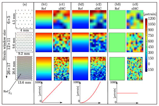
Figure 1.
Simulated strain distribution: (a) Discrete strain distribution showing measured points at the facets center for three strain windows with 6 × 5, 12 × 11 and 26 × 17 points which corresponds to a 4.5 × 4 mm, 9.6 × 9.2 mm, and 20.8 × 13.6 mm area, respectively. (b1–b3) Two-dimensional representation of linear, quadratic and constant simulated strain fields respectively. (c1–c3) strain distributions with imposed Gaussian noise obtained from digital image correlation (DIC) measured data points.
2.2. Experimental Strain Fields
Ten steel samples (mild steel 1.0037) were prepared according to ASTM guidelines for metallic materials (E8) [31] for tensile tests. Speckle patterns were applied to the steel samples’ surface using a high precision airbrush (Profi-AirBrush, Wiesbaden, Germany). The airbrush settings were adjusted (air pressure of 200 kPa, 3 turns of the airbrush opening, and 9 cm distance between the airbrush and the sample) to obtain a speckle size of 3–5 pixels [9] with a random distribution (coverage 45–50%). The samples were mounted on a Zwick (Z030) machine (ZwickRoell GmbH, Ulm, Germany). ARAMIS 3D commercial system (ARAMIS 150/6M/Rev.02, GOM GmbH, Braunschweig, Germany) was set up with two CCD cameras. The cameras were positioned perpendicular to the sample at 35 cm distance, see Figure 2a.
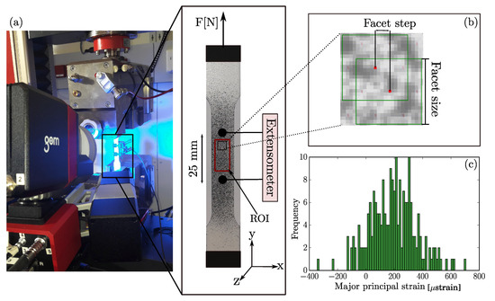
Figure 2.
(a) Tensile test setup. Steel samples were mounted on Z030 machine, an extensometer was attached to the sample and ARAMIS DIC system was capturing images of the test. ROI is the region of interest for DIC measurement points. (b) Facets and grid sizes. (c) Histogram of a strain field distribution at zero-strain for a facet size of 19 × 19 pixels and a facet step of 16 pixels.
The noise-floor of the DIC measurement was evaluated by capturing 10 images of each sample, at 1 Hz and 8 ms exposure time, while the sample was mounted on the testing machine without any load applied (zero-strain). The strain window corresponding to the measurement area between the extensometer has measurement points for a facet size of pixels with a facet step of 16 pixels (50% overlapping); these parameters are recommended by ARAMIS for 6 Megapixel CCD cameras [32], see Figure 2b in red as the region of interest (ROI). This pre-test was used to obtain reasonable noise levels for the simulated noise. The maximum noise at zero-load was less than strain, the average noise ranged from 140–210 strain and the standard deviation ranged from 200–270 strain for the 10 captured images (a value of 300 strain was taken as a worst case scenario and imposed on the simulated strain fields). The histograms of the strain measured were similar to Figure 2c. Finally, the steel samples were subjected to a uniaxial tensile load along the vertical direction with cross-head movement of 5 mm min until fracture. A universal extensometer (ZwickRoell GmbH, Germany) was attached to the samples in the gauge region (25 mm in length), from which the uniaxial global strain was obtained and referred to as reference strain (). The strain fields were subsequently exported from the ARAMIS Professional software (ARAMIS v6.3.1; GOM) as .csv file containing the node number, x-, y-, z-coordinates, and the measured strain values for plotting and post-processing with Python SciPy.
3. Filtering Approach
Three filtering approaches were applied on the strain fields: (1) simple mean filter which is also used in the DIC commercial software (ARAMIS v6.3.1; GOM), (2) Gaussian mean filter in the spatial domain which is used in Python SciPy. (3) A self-written script that implements Gaussian LPF in the frequency domain. In the following section, the difference between these filters is explained, as depicted in Figure 3. All three filters are in-house implementations.
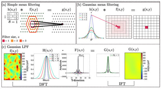
Figure 3.
Overview of the three filters approaches. (a) Simple mean filter, all measurement points at a specific distance are averaged together. (b) Gaussian mean filter, each measurement point is replaced with the mean value of its neighbours. (c) Gaussian low-pass filtering (LPF), by converting the measurement points into the frequency domain, an LPF can reduce the noise by eliminating high frequency components. Filtering is done on the measurement points and fields are shown for visualization purposes only.
The three filters have similar working principle, since the simple mean and Gaussian mean filtering perform convolution in spatial domain and differ only in two aspects; (a) the shape of the filter being ideal or Gaussian distributed; and (b) the shape of the kernel (hexagonal or square). Gaussian mean and Gaussian LPF are well alike, since convolution in the spatial domain is equivalent to multiplication in the frequency domain and vice versa [33]. Despite the similar working principle of these filters, differences in the results are observed.
3.1. Simple Mean Filter
This filter follows the implementation of an ARAMIS average filter and is implemented in Python 2.7. According ARAMIS/GOM guidelines [22], if the size (s) of the filter is 1, all points that are adjacent to the measurement point in a strain distribution will be averaged together and saved in a new filtered strain distribution , see Figure 3a for . Since DIC data are represented by a hexagonal grid, the shape of the filter is also hexagonal and all points are weighted equally. At the boundary, the strain points were extrapolated by reflecting the last three rows and columns.
3.2. Gaussian Mean Filter in Spatial Domain
Gaussian mean filtering replaces the value of each pixel in an image plane with the mean value of its neighbours including the pixel itself [33], see Figure 3b. The shape of the filter weight the pixels based on their distance to the measured point.
where are the coordinates of a measurement point in a 2D strain distribution, and is the standard deviation of a Gaussian function. The filtering is applied via convolution . During optimization, a Gaussian mean filter was applied with to 10 with increment using a built-in function in Python.
3.3. Gaussian Lpf in Frequency Domain
Filtering in the frequency domain is recommended, since the noise is represented by a high frequency component [28]. In this study, a Gaussian LPF [33], , was applied:
where is the distance of point from the center of the spectrum, and is the cutoff frequency of the filter that controls the shape of the Gaussian. Basic steps of filtering in the frequency domain are, see Figure 3c:
- (a)
- The strain distribution is transformed from the spatial domain into the frequency domain, , using discrete Fourier transform (DFT).
- (b)
- The obtained spectrum from DFT is shifted to the center by multiplying with , to locate the low frequency peaks at the center of the image .
- (c)
- A Gauss LPF, , with to 10 with increment, is multiplied with the centered spectrum .
- (d)
- Using inverse Fourier transform (IFT), is transformed back to the spatial domain , and the real part of this inversion is shifted again by .
3.4. Error Reduction of Full-Field Strain Evaluation
The filtering efficiency is measured by two terms of error; the loss of information and the residual noise. The loss of information is the amount of true signal lost when the reference strains at measurement points () were filtered () Equation (3). The residual noise is the distance between each reference point () and filtered noisy point () for each stage (see Equation (4) and Figure 4). The total error is the square-root of the sum of the quadratic of both error terms Equation (5) [28]. The reference strain is either null in the case of zero-strain or the simulated strain field without noise imposed, or is the global strain determined from the extensometer in case of the loaded steel samples. The error was calculated as the RMSE with the following equations.
where n is the number of local strain measurement points (i), e.g., computed by ARAMIS, is the value of the reference strain, is the value of the filtered reference strain, and is the value of the filtered noisy point. Smaller RMSE means better denoising. The error reduction is described by how good the noise elimination is and was calculated as following:
where the imposed noise is strains for simulated cases. Ideally, the total error is zero and the error reduction is at its maximum. The error reduction increases with decreasing total error.
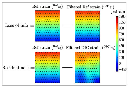
Figure 4.
Overview of the RMSE calculations. Fields are only shown for visualization; calculations are done by using the measurement points. The loss of information is defined as the difference between the reference field and the filtered reference field (top row). The residual noise is defined as the difference between the reference field and the filtered noisy field.
The optimal specific filter parameters were found as the filter parameter that had the minimum total error for each strain window size. The overall optimal filter parameters were calculated as the mean of the optimal specific filter values from the linear and quadratic fields, as per the following equation:
where j is the number of strain windows. Parameters obtained from constant strain fields are neglected because finding an optimal filter in such cases is not meaningful for higher-order strain fields.
4. Results
4.1. Simulated Strain Fields
Figure 5, Figure 6 and Figure 7 show the influence of filtering on the loss of information, residual noise and total error, respectively. The loss of information increases with changing the filter size for both the simple means and the Gauss mean filtering, while it decreases for Gauss LPF, as depicted in Figure 5c,c1. The residual noise increases for the simple mean filtering for the smallest window size, and it increases sharply for Gauss mean filtering and mildly for Gauss LPF, as depicted in Figure 6b–c1. The optimal filtering parameters were found based on the total error curve, as depicted in Figure 7; the opaque pink bar shows the range of the optimal filtering parameters, which was determined where the total error had a minimum for each strain window and field type. Figure 8 shows the corresponding linear and quadratic strain fields with the specific filtering parameters for each strain window and the overall optimal filtering parameter.
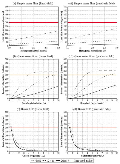
Figure 5.
Curves of loss of information for different strain window sizes for linear and quadratic strain fields. The unit of the kernel size (s), standard deviation (), and cutoff frequency () is measurement points.
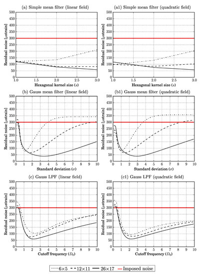
Figure 6.
Curves of residual noise for different strain window sizes for linear and quadratic strain fields. The unit of the kernel size (s), standard deviation (), and cutoff frequency () is measurement points.
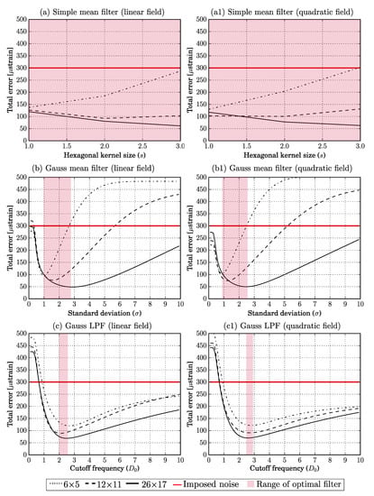
Figure 7.
Curves of total error for different strain window sizes for linear and quadratic strain fields. The opaque pink bar shows the range of the optimal filtering parameters.The unit of the kernel size (s), standard deviation (), and cutoff frequency () is measurement points.
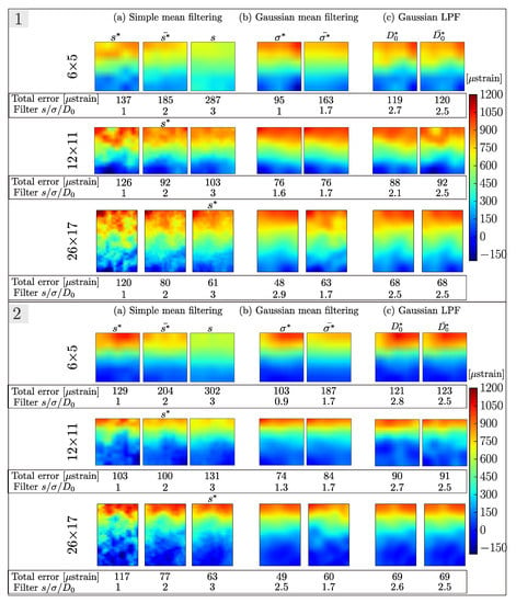
Figure 8.
Two-dimensional visualization of (1) linear and (2) quadratic strain fields (a) Simple mean filter for s = 1, 2, and 3, (b) Gaussian mean filter with for each strain window and = 1.7, (c) Gaussian LPF with for each strain window and = 2.5.
The simple mean filter shows a considerable influence of the size s for different strain window sizes and types (Figure 7a,a1). Graphically, this is also visible in Figure 8a. A good compromise is found with , with an error reduction of 38, 69 and for linear fields and 32, 66 and for the quadratic fields for the different sizes of the strain windows.
The range of the specific filter parameter for Gaussian mean filtering was from 1 to for the linear fields and from to for the quadratic fields as depicted in Figure 7b,b1 with overall filtering parameter . The corresponding strain fields (Figure 8b), for and show less error compared to simple mean filtering and Gaussian LPF, except for the quadratic field when was applied. Applying , Gaussian mean filtering reconstructed the linear fields with error reduction of 45, 74 and , and the quadratic fields with error reduction of 37, 72 and for the different sizes of the strain windows.
Gaussian LPF had between and for linear fields and between and for the quadratic fields; see Figure 7c,c1 with overall filtering parameter . Applying , Gaussian LPF reconstructed the linear fields with error reduction of , and , and the quadratic fields with error reduction of , and for the different sizes of the strain windows. Figure 8 shows a 2D visualization of the filtered strain fields.
The application of , , and to the constant simulated strain fields are summarized in Figure 9, where the error reduction for different strain window sizes is shown. Regardless of the size of the strain windows, Gaussian mean filtering performs best (error reduction 73–81%) whereas for a window size of and , Gaussian LPF performs at least with error reduction of . For a window size of , all filters achieved a similar level of error reduction.
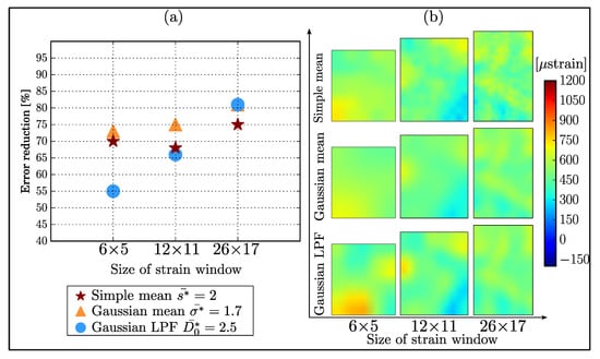
Figure 9.
Error reduction achieved for simulated constant strain fields (a) Percentage of error reduced for the different sizes of the strain windows and the filters, (b) Two-dimensional visualization of the filtered constant strain fields.
An overview of error reduction achieved for a selected strain window of points is summarized in Table 1.

Table 1.
Achieved error reduction for simulated strain fields and filtering approaches for a 12 × 11 strain window.
4.2. Experimental Strain Fields
For samples deforming under tensile load, the size of the strain window was about measurement points and the noise had an RMSE amplitude of ± to ± strain independent of the load level. The reference strain measurements, DIC strain measurements and its standard deviation for the four load levels are presented in Table 2.

Table 2.
Reference strain (measured by the extensometer) vs. DIC strain and standard deviation measured on the surface of steel samples under tensile load.
The overall optimal filters (, , ) were applied on the strain windows from the steel samples. The total error and the error reduction level are depicted in Figure 10a at four loading steps 500, 1500, 2000 and 3000 N load, Figure 10b shows the corresponding 2D interpolated strain fields overlaid with the discrete measurement points. The total error was reduced by 50% when applying the three overall optimal parameters, without any remarkable difference with regards to the load level.
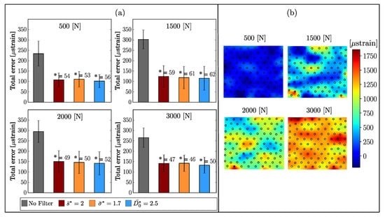
Figure 10.
(a) Total error and accuracy of filtering a 12 × 11 stain window of steel samples. (b) Two-dimensional interpolated strain fields overlaid with the discrete measurement points. Both presented at 500, 1500, 2000, and 3000 N load steps. No Filter is the raw DIC measurement points.
5. Discussion
The goal of this study was to examine three practical filtering approaches, to compare their effectiveness on three simulated strain fields (linear, quadratic, and constant) where the ’True’ reference strain is known, to find optimal filter parameters with minimum compromising between residual noise and loss of information, and to apply such filters to experimental strain fields. A simple mean with , a Gaussian mean with , and a Gaussian LPF with were identified as the overall optimal filter parameters for the examined strain window size and strain field type. These filters give at least an error reduction above , and for simulated fields and an error reduction above , and for experimental fields.
On the one hand, the Gaussian mean filtering is outstanding in terms of error reduction for constant strain windows (Figure 9). On the other hand, for linear and quadratic strain windows (Figure 7), the shape of the total error curve shows high gradients around the minimum point, which implies a sharper increase in the total error when deviating from the specific optimal . The increase in total error (Figure 8) from when to was applied is around 75 strain for the smallest () strain window size, and about 12 strain for the other strain window sizes. The same can be seen for the loss of information and residual noise Figure 5b,b1 and Figure 6b,b1, respectively.
The Gaussian LPF behaved based on the shape of the strain window rather than the size. For homogeneous/constant strain field, the noise can be filtered using a , by letting only the smallest frequency pass and blocking all higher frequency components, as this might work well for homogeneous/constant fields. This does not work for linear and quadratic fields and will result in a corrupted strain distribution, as confirmed as well by Baldoni et al. [28] with total error, in our case, higher than the original noise (Figure 7c,c1). As well, when applying filtering on the speckled DIC image prior to the correlation calculation, Butterworth LPF produced the lowest random error [30]. The Gaussian LPF was the only filter where the loss of information was reduced with increased cutoff frequency. This is because the reference strain—in case of the simulated fields—is noiseless, and when increasing the cutoff frequency, the whole signal passed, allowing the filtered field to be identical to the original field. However, for the residual noise, with increasing the cutoff frequency, the noise remaining in the filtered field is increasing mildly, as depicted in Figure 6c,c1.
These three overall optimal parameters that reduced the noise in both the simulated and the experimental fields can be used, for comparable strain window sizes, when no prior information is available on the strain field. Simple mean filtering is handy since it is a built-in function that comes usually with commercial DIC systems, but for the smallest strain window points (Figure 8, top, left)—if the optimal filter size was not used—a serious compromise of the results can occur, with noise reduction from 300 to strains. If the overall optimal parameter was used, the noise reduction is limited to and for the linear and quadratic fields, respectively.
It was demonstrated here how the size of the strain window influences the noise reduction, better denoising is achieved for bigger strain window sizes [17,34,35], which is expected, since for bigger stain windows, more facets can be calculated and the signal to noise ratio is higher than for smaller strain windows. This can be seen clearly in the total error curves in Figure 7, where the minimum and maximum total error were reached for the and strain windows, respectively. Filtering, either on the displacement field, the strain fields or the speckled images, helps reducing noise in DIC fields [12,19,28,30], but the optimization of other factors that influence the noise is necessary, such as facet and step size. For facet size; a bigger facet size results in better identification of the facets and is favoured for the correlation algorithm [17,36,37]. Other studies showed that the error can be largely reduced by increasing the facet size [6,38]. However, since we seek to improve DIC measurements for non-homogenous specimens or for specimens with geometry that allow strain concentration, choosing a bigger facet size is not ideal and would lead to hide the strain concentrations. For our case, with a fixed dimensions of the strain fields between the extensometer, more data points can be measured with smaller facet size and/or step, but at the cost of more noise which was confirmed by other studies [6,11,21,39]. When the facet size was set to be pixels with pixels facet step, the RMSE doubled from 300 to 600 strains with maximum apparent strain exceeding 1000 strains, thus, when non-homogenous strain concentration is expected, a good compromise is needed between a larger facet size to suppress the noise and a smaller one to capture the strain concentration.
As a general DIC filtering guideline, filters available by the DIC commercial software or by a computational software such as Python can be useful in reducing the noise in DIC fields. However, as demonstrated above, the selection of the filter parameter should be based on an optimization process to ensure the minimum loss of information and the preservation of the strain gradient. The concept of the total error as a combination of the loss of information and residual noise is a powerful tool to see the influence of each filter on the DIC measured data points. When applying filters provided by a commercial DIC software, it is important to keep in mind the relation between the filter parameter and the size of the strain field.
The limitations of this study are that specific simulated strain fields were tested and the experimental results represent only homogeneous strain fields. In future, it has to be proven that the presented approach works also for real measured higher-order strain fields. Only strain window sizes up to points ( mm) are considered, since smaller strain windows sizes are influenced by higher noise. One length scale of the noise was investigated in this study, which was obtained from the experimental findings. Additionally, filtering was applied directly on strain field measurement points obtained from the software i.e. no filtering on displacement fields, no investigation on different strain computation methods, or different correlation algorithms, such as global and local DIC approaches, were investigated in this study. Finally, optimal filtering parameters presented here might not be optimal for other applications with different DIC systems or at different length scales.
6. Conclusions
DIC offers a method for capturing full-field deformation on the surface of the samples, regardless of their size, shape or material. With appropriate analysis parameters, DIC can capture the strain on the surface of tested samples. The present study has illustrated that strain computed by DIC commercial software (ARAMIS v6.3.1; GOM) is comparable to strains obtained from a high precision extensometer attached to the same sample. The DIC noise was stable over the different load levels in the elastic deformation region of the material.
However, DIC measurement cannot be taken for granted without checking the noise-floor; thus, preliminary tests at zero-strain can give an idea on the noise-floor of the measurement due to software or hardware parameters. Few studies focus on filtering the strain fields, in this study a procedure to select an optimal filter parameters has been presented. The results found in this study show that optimal filtering can have a positive effect on reducing the noise, but at the cost of losing information, especially for simple mean and Gauss mean filters. Optimal Gauss LPF proved to be effective in reducing the noise without excessive loss of information. This effect can only be shown by using simulated strain fields where a noiseless reference strain field is known. When filtering DIC measurement on sample with irregular shape or non-homogenous material such as bone, practical filtering guidelines as given in this study can be very helpful.
Author Contributions
Conceptualization, N.A. and D.H.P.; methodology, N.A., A.R. and D.H.P.; software, D.H.P.; validation, N.A., A.R. and D.H.P.; formal analysis, N.A.; investigation, N.A.; resources, N.A.; data curation, N.A.; writing—original draft preparation, N.A.; writing—review and editing, N.A., A.R. and D.H.P.; visualization, N.A.; supervision, A.R. and D.H.P.; project administration, D.H.P.; funding acquisition, N.A. and D.H.P. All authors have read and agreed to the published version of the manuscript.
Funding
The authors disclosed receipt of financial support from the Niederoesterreiche Forschung and Buildung (NFB) Institute via the Dissertation scholarship 2018 [grant number SC18-006] for the research of this article. The authors acknowledge TU Wien Bibliothek for financial support through its Open Access Funding Program.
Conflicts of Interest
The authors declare no conflict of interest.
Appendix A
The working principle of DIC is based on comparing two digital images of the surface of interest acquired in undeformed (reference) and deformed state. Through this comparison, DIC can provide full-field displacements to sub-pixel accuracy. For tracking the displacement on the surface of the sample using a DIC system (in this study Aramis commercial system is used), the surface of test samples has to be sprayed with random speckle patterns. The surface is divided into facets of pixels; the centers of theses facets are known as measurement points Figure A1a. Each facet is has a unique grey-value distribution of pixels and location in space. The facets are identified and matched along the image series using the method of image correlation. The best matching region of the two images, where the maximum correlation coefficient is found, is taken as the new position of the measurement point [1,3,22,28]. After defining the coordinates of the points in the reference image and in the image of the deformed state, displacements in x-, y- and z-direction can be computed as the difference between the deformed and the reference states, e.g., x-, y- or z-.
For three-dimensional computation (3D), two cameras are needed to be able to calculate the coordinates in the deformed stage via triangulation. Strains are calculated from the obtained displacements, similar as in finite element methods [22]. A triangular mesh is placed onto the ROI, with the nodes being the measurement points where the displacements were computed, see Figure A1b, the coordinates of the reference image correspond to A, B and 0, forming one triangular element.
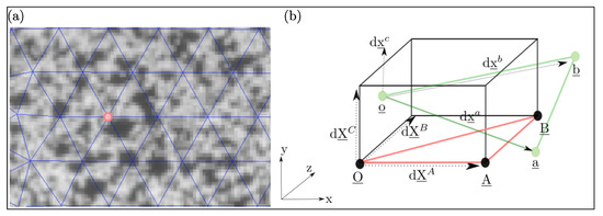
Figure A1.
(a) Measurement point (center of facets) on a speckled surface. (b) Background of displacement computation, displacements of each measurement point is computed in x-, y- and z-direction.
The deformation gradient is computed as in the following Equation (A1)
where F is the deformation gradient, dx and dX are the position of a measurement point in the deformed and reference position respectively. The position of the measurement point in the deformed state is the position of the measurement point in the reference state plus the displacement, as per the following equation
where du is the displacement gradient. The movement and deformation of an element (O, A, B) can be computed based on the movement of its points and can be described as following for point A
Since the point distribution is based on triangles (see Figure A1a), one needs at least three points with known undeformed and deformed coordinates for computing the displacement and the deformation. The Green–Lagrange strain tensor can be computed as per the following equation
From the strain tensor, specific strains in x-, y- and z-direction of an element can be obtained and assigned to the measurement point.
References
- Sutton, M.A.; Orteu, J.J.; Schreier, H. Image Correlation for Shape, Motion and Deformation Measurements: Basic Concepts, Theory and Applications; Springer Science & Business Media: New York, NY, USA, 2009. [Google Scholar]
- Tong, W. An evaluation of digital image correlation criteria for strain mapping applications. Strain 2005, 41, 167–175. [Google Scholar] [CrossRef]
- Sztefek, P.; Vanleene, M.; Olsson, R.; Collinson, R.; Pitsillides, A.A.; Shefelbine, S. Using digital image correlation to determine bone surface strains during loading and after adaptation of the mouse tibia. J. Biomech. 2010, 43, 599–605. [Google Scholar] [CrossRef] [PubMed]
- Gustafson, H.; Siegmund, G.; Cripton, P. Comparison of strain rosettes and digital image correlation for measuring vertebral body strain. J. Biomech. Eng. 2016, 138, 054501. [Google Scholar] [CrossRef] [PubMed]
- Hensley, S.; Christensen, M.; Small, S.; Archer, D.; Lakes, E.; Rogge, R. Digital image correlation techniques for strain measurement in a variety of biomechanical test models. Acta Bioeng. Biomech. 2017, 19. [Google Scholar] [CrossRef]
- Acciaioli, A.; Lionello, G.; Baleani, M. Experimentally Achievable Accuracy Using a Digital Image Correlation Technique in measuring Small-Magnitude (less than 0.1%) Homogeneous Strain Fields. Materials 2018, 11, 751. [Google Scholar] [CrossRef]
- Perry, C. Strain-Gage Reinforcement Effects on Orthotropic Materials. Exp. Tech. 1986, 10, 20–24. [Google Scholar] [CrossRef]
- Cristofolini, L.; Schileo, E.; Juszczyk, M.; Taddei, F.; Martelli, S.; Viceconti, M. Mechanical testing of bones: The positive synergy of finite–element models and in vitro experiments. Philos. Trans. R. Soc. Lond. Math. Phys. Eng. Sci. 2010, 368, 2725–2763. [Google Scholar] [CrossRef][Green Version]
- Lecompte, D.; Bossuyt, S.; Cooreman, S.; Sol, H.; Vantomme, J. Study and generation of optimal speckle patterns for DIC. In Proceedings of the Annual Conference and Exposition on Experimental and Applied Mechanics, Springfield, MA, USA, 3–6 June 2007; pp. 1643–1649. [Google Scholar]
- Barranger, Y.; Doumalin, P.; Dupré, J.; Germaneau, A. Digital Image Correlation Accuracy: Influence of Kind of Speckle and Recording Setup; EDP Sciences: Les Ulis, France, 2010; Volume 6, p. 31002. [Google Scholar]
- Wang, Y.; Lava, P.; Coppieters, S.; De Strycker, M.; Van Houtte, P.; Debruyne, D. Investigation of the uncertainty of DIC under heterogeneous strain states with numerical tests. Strain 2012, 48, 453–462. [Google Scholar] [CrossRef]
- Rajan, V.; Rossol, M.; Zok, F. Optimization of digital image correlation for high-resolution strain mapping of ceramic composites. Exp. Mech. 2012, 52, 1407–1421. [Google Scholar] [CrossRef]
- Mortazavi, F. Development of a Global Digital Image Correlation Approach for Fast High-Resolution Displacement Measurements. Ph.D. Thesis, École Polytechnique de Montréal, Montréal, QC, Canada, 2013. [Google Scholar]
- Lionello, G.; Cristofolini, L. A practical approach to optimizing the preparation of speckle patterns for digital-image correlation. Meas. Sci. Technol. 2014, 25, 107001. [Google Scholar] [CrossRef]
- Lionello, G.; Sirieix, C.; Baleani, M. An effective procedure to create a speckle pattern on biological soft tissue for digital image correlation measurements. J. Mech. Behav. Biomed. Mater. 2014, 39, 1–8. [Google Scholar] [CrossRef] [PubMed]
- Palanca, M.; Tozzi, G.; Cristofolini, L. The use of digital image correlation in the biomechanical area: A review. Int. Biomech. 2016, 3, 1–21. [Google Scholar] [CrossRef]
- Yaofeng, S.; Pang, J.H. Study of optimal subset size in digital image correlation of speckle pattern images. Opt. Lasers Eng. 2007, 45, 967–974. [Google Scholar] [CrossRef]
- Xavier, J.; Sousa, A.M.; Morais, J.J.; Filipe, V.M.; Vaz, M.A. Measuring displacement fields by cross-correlation and a differential technique: Experimental validation. Opt. Eng. 2012, 51, 043602. [Google Scholar] [CrossRef]
- Avril, S.; Feissel, P.; Pierron, F.; Villon, P. Comparison of two approaches for differentiating full-field data in solid mechanics. Meas. Sci. Technol. 2009, 21, 015703. [Google Scholar] [CrossRef]
- Hild, F.; Roux, S. Comparison of local and global approaches to digital image correlation. Exp. Mech. 2012, 52, 1503–1519. [Google Scholar] [CrossRef]
- Wang, B.; Pan, B. Subset-based local vs. finite element-based global digital image correlation: A comparison study. Theor. Appl. Mech. Lett. 2016, 6, 200–208. [Google Scholar] [CrossRef]
- GOM-GmbH. Digital Image Correlation and Strain Computation Basics; GOM-GmbH: Gomadingen, Germany, 2016. [Google Scholar]
- Geers, M.; De Borst, R.; Brekelmans, W. Computing strain fields from discrete displacement fields in 2D-solids. Int. J. Solids Struct. 1996, 33, 4293–4307. [Google Scholar] [CrossRef][Green Version]
- Rubino, V.; Lapusta, N.; Rosakis, A.; Leprince, S.; Avouac, J. Static laboratory earthquake measurements with the digital image correlation method. Exp. Mech. 2015, 55, 77–94. [Google Scholar] [CrossRef]
- Sun, Y.; Pang, J.H.; Wong, C.K.; Su, F. Finite element formulation for a digital image correlation method. Appl. Opt. 2005, 44, 7357–7363. [Google Scholar] [CrossRef]
- Rubino, V.; Rosakis, A.; Lapusta, N. Full-field ultrahigh-speed quantification of dynamic shear ruptures using digital image correlation. Exp. Mech. 2019, 59, 551–582. [Google Scholar] [CrossRef]
- Mortazavi, F.; Levesque, M.; Villemure, I. Image-based Continuous Displacement Measurements Using an Improved Spectral Approach. Strain 2013, 49, 233–248. [Google Scholar] [CrossRef]
- Baldoni, J.; Lionello, G.; Zama, F.; Cristofolini, L. Comparison of different filtering strategies to reduce noise in strain measurement with digital image correlation. J. Strain Anal. Eng. Des. 2016, 51, 416–430. [Google Scholar] [CrossRef]
- Pan, B. Bias error reduction of digital image correlation using Gaussian pre-filtering. Opt. Lasers Eng. 2013, 51, 1161–1167. [Google Scholar] [CrossRef]
- Zhou, Y.; Sun, C.; Song, Y.; Chen, J. Image pre-filtering for measurement error reduction in digital image correlation. Opt. Lasers Eng. 2015, 65, 46–56. [Google Scholar] [CrossRef]
- International, A. E8, Standard Test Methods for Tension Testing of Metallic Materials. Annu. Book Astm Stand. 2004, 3, 57–72. [Google Scholar]
- GOM-GmbH. Acquisition Basic: GOM Software 2016; GOM-GmbH: Gomadingen, Germany, 2015. [Google Scholar]
- Gonzalez, R.C.; Woods, R.E. Digital Image Processing, 2nd ed.; Addison-Wesley Longman Publishing Co., Inc.: Boston, MA, USA, 1992. [Google Scholar]
- Cofaru, C.; Philips, W.; Van Paepegem, W. A novel speckle pattern—Adaptive digital image correlation approach with robust strain calculation. Opt. Lasers Eng. 2012, 50, 187–198. [Google Scholar] [CrossRef]
- Pan, B.; Yuan, J.; Xia, Y. Strain field denoising for digital image correlation using a regularized cost-function. Opt. Lasers Eng. 2015, 65, 9–17. [Google Scholar] [CrossRef]
- Lecompte, D.; Smits, A.; Bossuyt, S.; Sol, H.; Vantomme, J.; Van Hemelrijck, D.; Habraken, A.M. Quality assessment of speckle patterns for digital image correlation. Opt. Lasers Eng. 2006, 44, 1132–1145. [Google Scholar] [CrossRef]
- Cofaru, C.; Philips, W.; Van Paepegem, W. Improved Newton—Raphson digital image correlation method for full-field displacement and strain calculation. Appl. Opt. 2010, 49, 6472–6484. [Google Scholar] [CrossRef]
- Pan, B.; Tian, L. Advanced video extensometer for non-contact, real-time, high-accuracy strain measurement. Opt. Express 2016, 24, 19082–19093. [Google Scholar] [CrossRef] [PubMed]
- Palanca, M.; Brugo, T.M.; Cristofolini, L. Use of digital image correlation to investigate the biomechanics of the vertebra. J. Mech. Med. Biol. 2015, 15, 1540004. [Google Scholar] [CrossRef]
© 2020 by the authors. Licensee MDPI, Basel, Switzerland. This article is an open access article distributed under the terms and conditions of the Creative Commons Attribution (CC BY) license (http://creativecommons.org/licenses/by/4.0/).