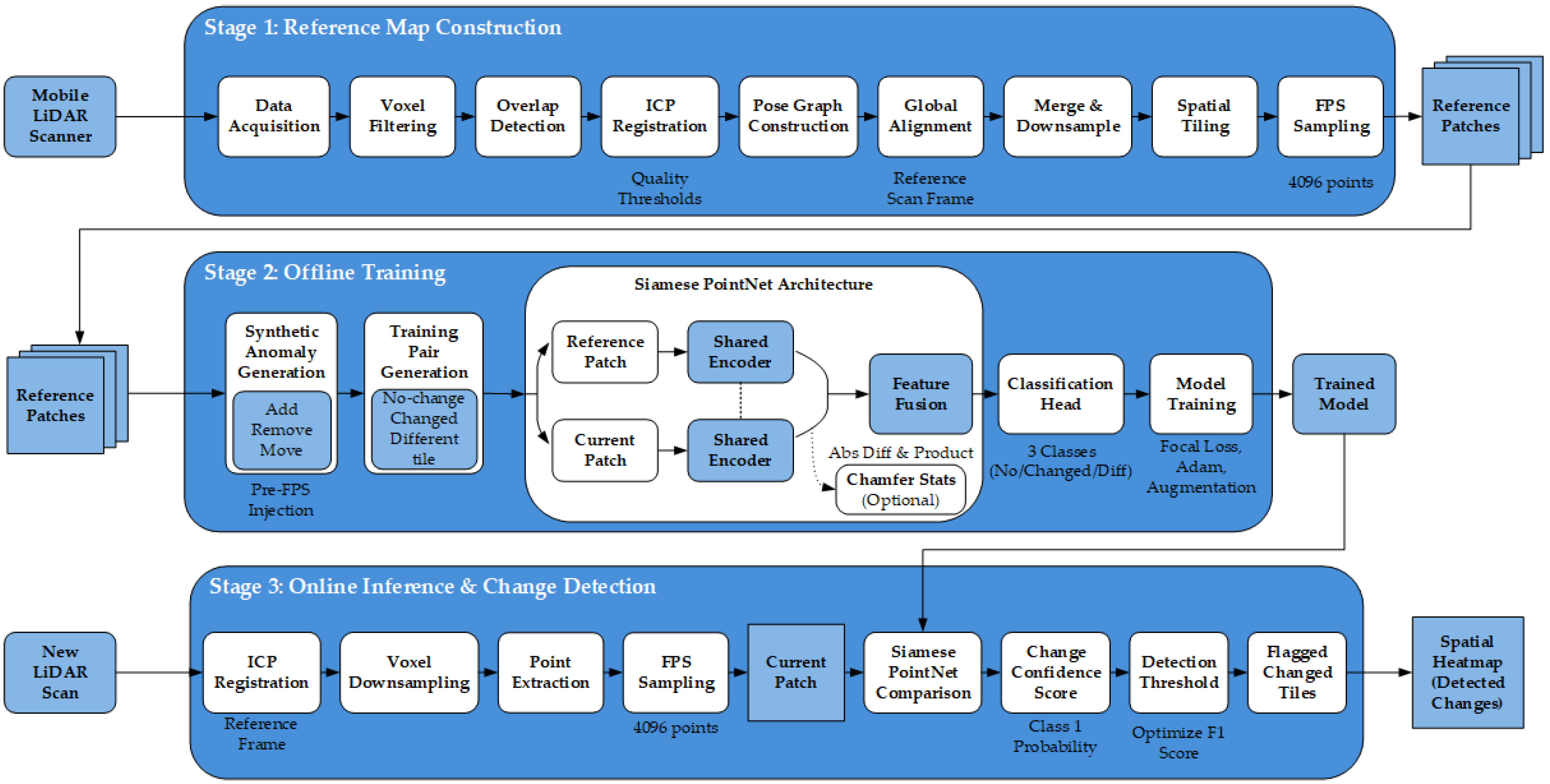
Figure 1.
System overview of the autonomous indoor 3D change detection framework. Stage 1 constructs the reference map using the automated mobile LiDAR registration pipeline presented in [
26]. Stage 2 trains a three-class Siamese PointNet classifier on synthetically generated change pairs. Stage 3 deploys the trained model for lightweight online tile-level change detection from new LiDAR scans.
Figure 1.
System overview of the autonomous indoor 3D change detection framework. Stage 1 constructs the reference map using the automated mobile LiDAR registration pipeline presented in [
26]. Stage 2 trains a three-class Siamese PointNet classifier on synthetically generated change pairs. Stage 3 deploys the trained model for lightweight online tile-level change detection from new LiDAR scans.
Figure 2.
Fused global reference map generated from registered LiDAR scans of the indoor corridor environment, with visualization of voxel-downsampled geometry and the spatial tile grid used for patch extraction. (a) Top-down view (XY) of the voxel-downsampled map (5 cm resolution) with height-based coloring. (b) Spatial tile grid overlay showing valid tiles (blue, 1.5 × 1.5 × 1.0 m). (c) Side view (XZ) showing the vertical extent and tile height.
Figure 2.
Fused global reference map generated from registered LiDAR scans of the indoor corridor environment, with visualization of voxel-downsampled geometry and the spatial tile grid used for patch extraction. (a) Top-down view (XY) of the voxel-downsampled map (5 cm resolution) with height-based coloring. (b) Spatial tile grid overlay showing valid tiles (blue, 1.5 × 1.5 × 1.0 m). (c) Side view (XZ) showing the vertical extent and tile height.
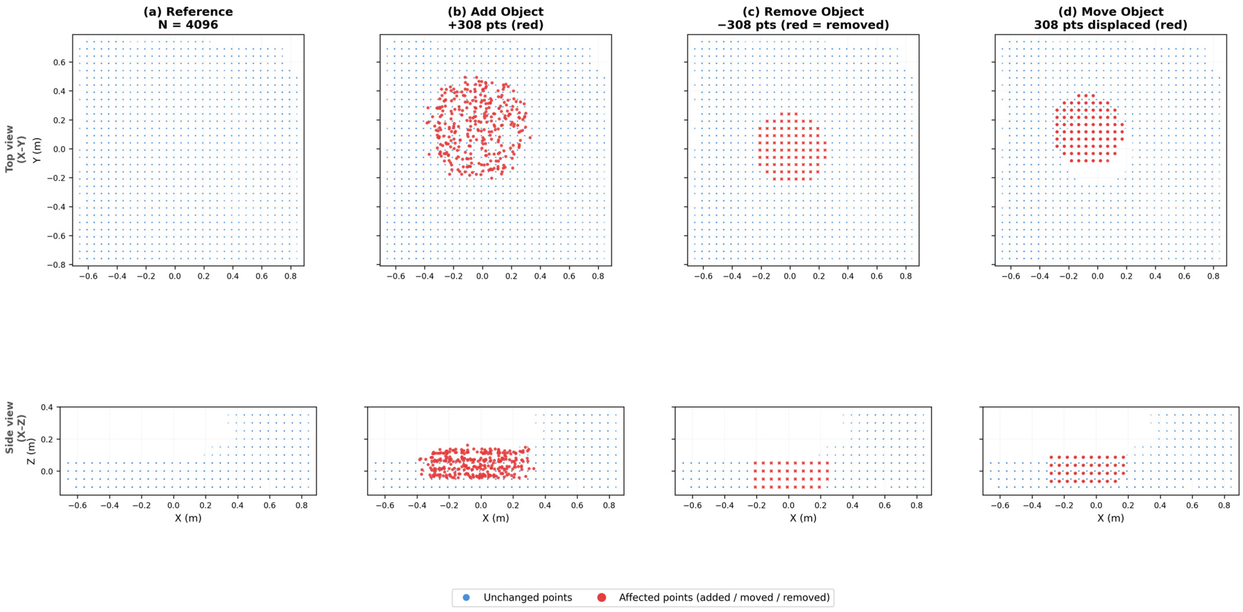
Figure 3.
Examples of synthetic anomaly operations applied to a reference tile (N = 4096), illustrating how geometric changes are injected into dense point clouds prior to FPS subsampling. (a) Reference tile before anomaly injection. (b) Add operation: new points are duplicated and displaced to simulate object appearance. (c) Remove operation: points are deleted to simulate object disappearance. (d) Move operation: points are translated to simulate object displacement.
Figure 3.
Examples of synthetic anomaly operations applied to a reference tile (N = 4096), illustrating how geometric changes are injected into dense point clouds prior to FPS subsampling. (a) Reference tile before anomaly injection. (b) Add operation: new points are duplicated and displaced to simulate object appearance. (c) Remove operation: points are deleted to simulate object disappearance. (d) Move operation: points are translated to simulate object displacement.
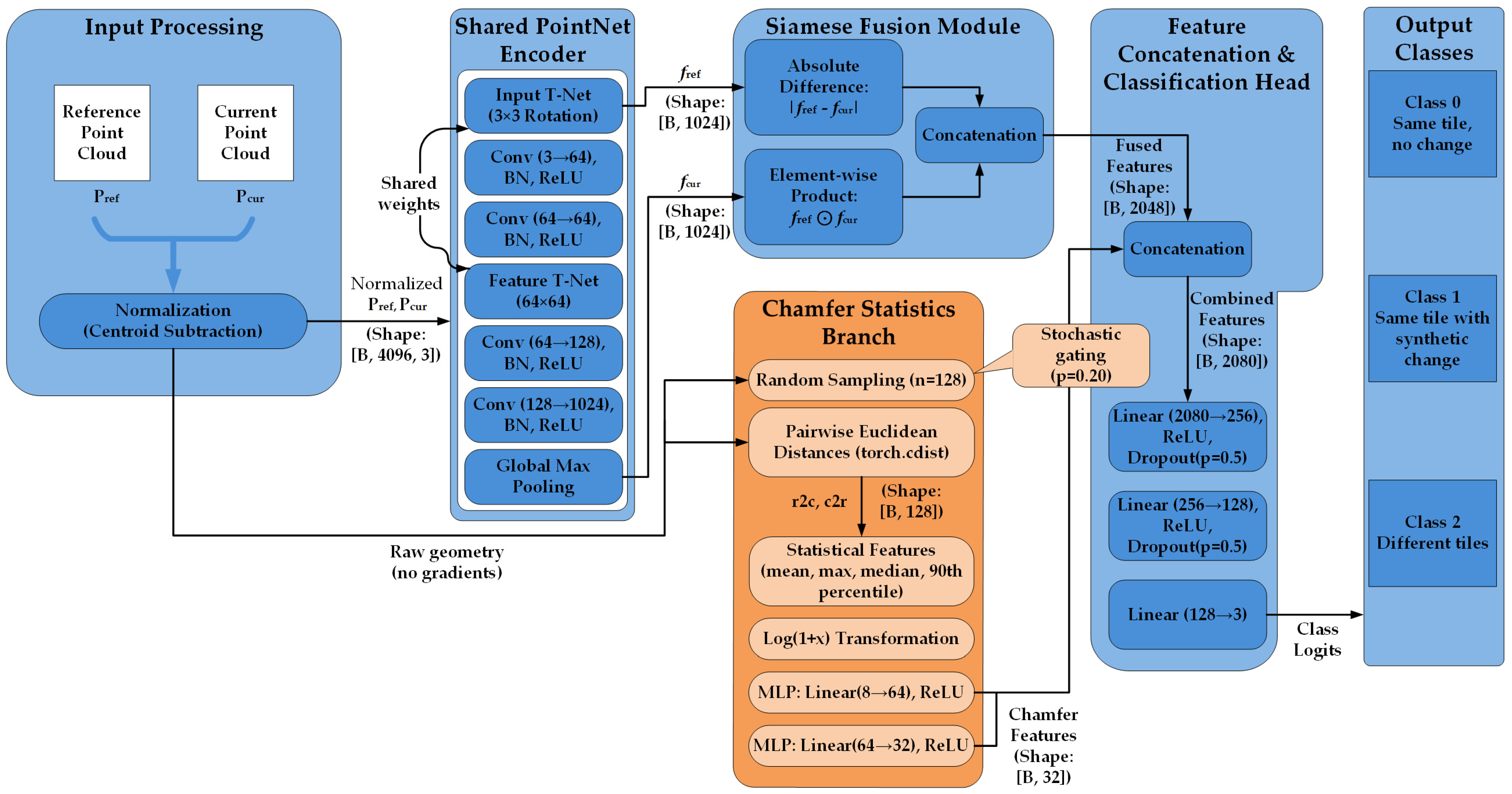
Figure 4.
SPICD-Net architecture with Chamfer statistics branch and stochastic gating, showing shared-weight encoders, feature fusion strategy, and the classification head for three-class tile-level change detection.
Figure 4.
SPICD-Net architecture with Chamfer statistics branch and stochastic gating, showing shared-weight encoders, feature fusion strategy, and the classification head for three-class tile-level change detection.
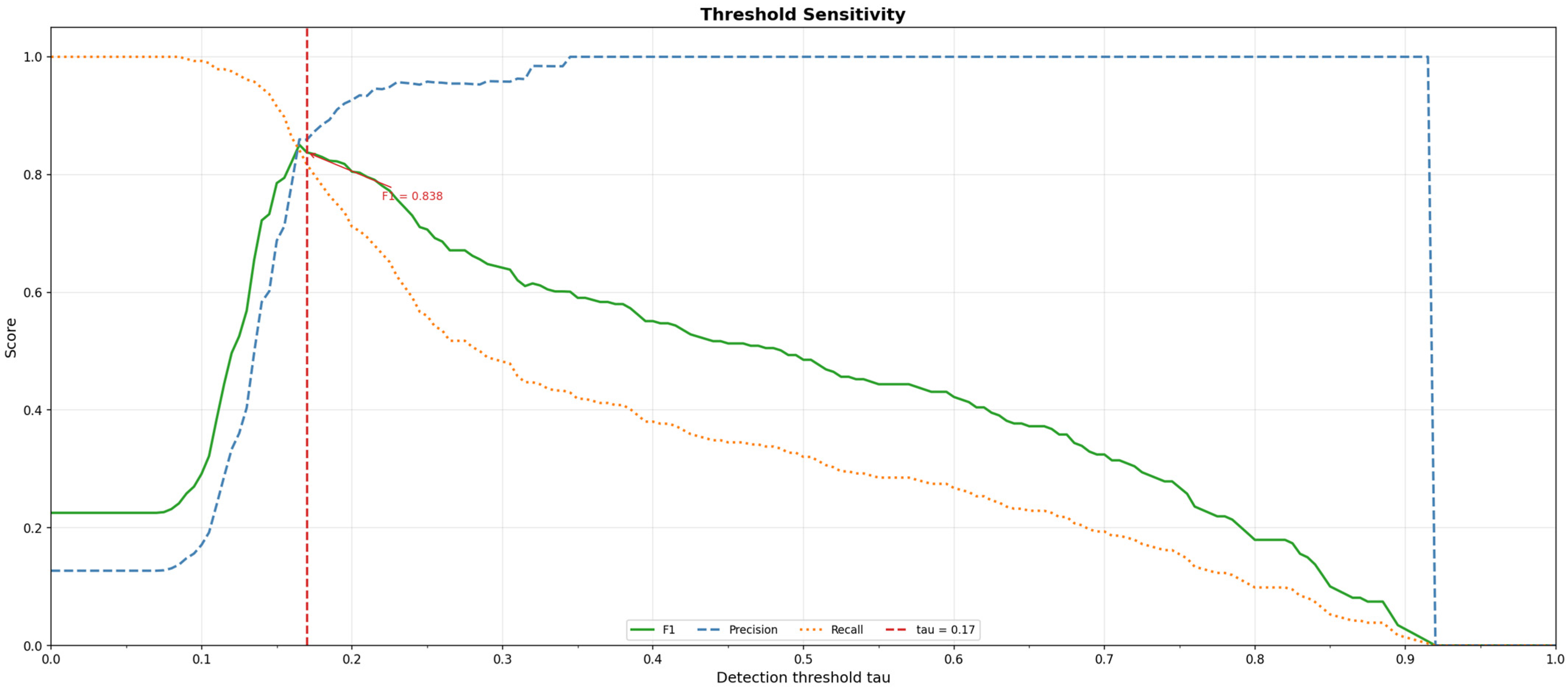
Figure 5.
Threshold sensitivity of precision, recall, and F1-score as a function of detection threshold τ. The selected operating threshold τ = 0.17 (dashed red line) coincides with the F1 peak. The F1 curve remains within 0.01 of its maximum across the range τ ∈ [0.12, 0.22], confirming that performance is not sensitive to the exact threshold choice in this region.
Figure 5.
Threshold sensitivity of precision, recall, and F1-score as a function of detection threshold τ. The selected operating threshold τ = 0.17 (dashed red line) coincides with the F1 peak. The F1 curve remains within 0.01 of its maximum across the range τ ∈ [0.12, 0.22], confirming that performance is not sensitive to the exact threshold choice in this region.
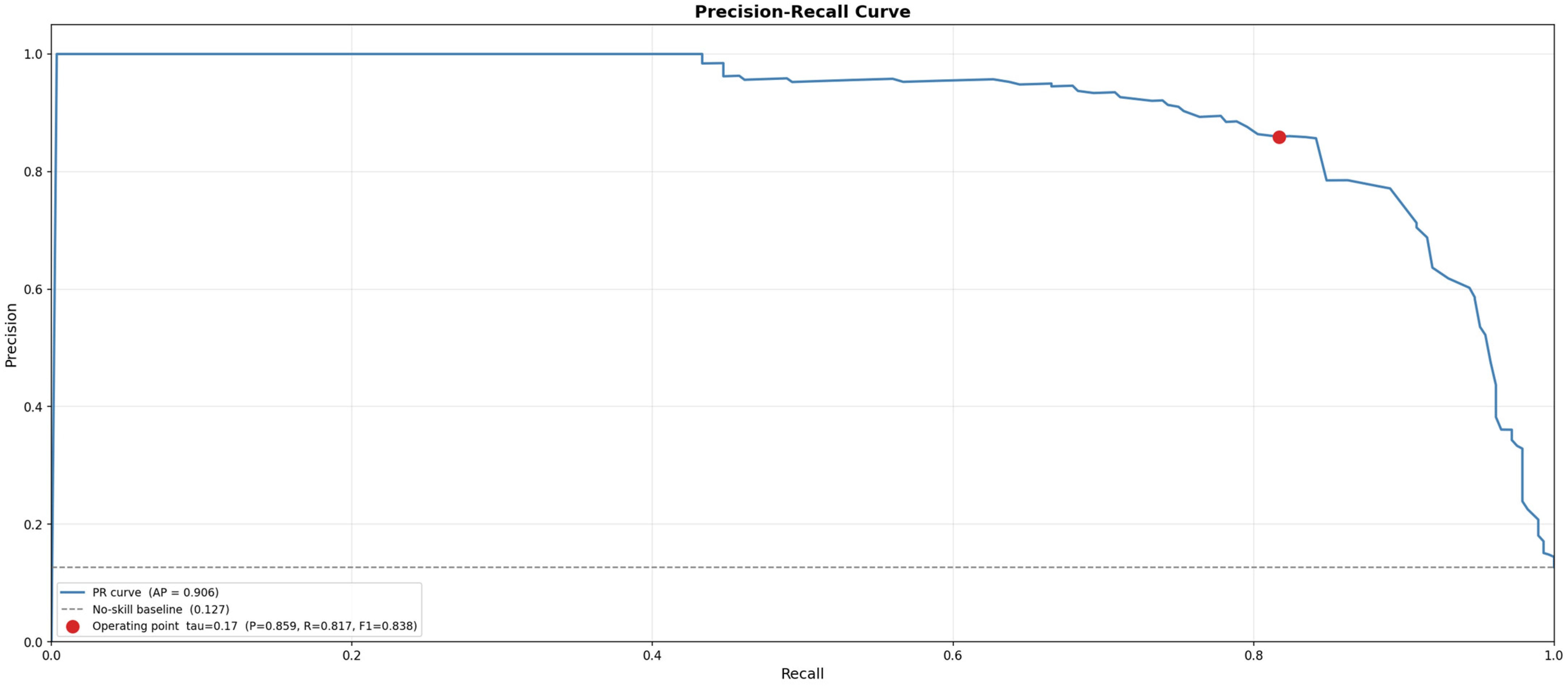
Figure 6.
Precision–recall curve for tile-level change detection across the simulation benchmark. The marked operating point at τ = 0.17 shows the selected thresholded evaluation, while the overall curve provides a threshold-independent view of detection performance under class imbalance.
Figure 6.
Precision–recall curve for tile-level change detection across the simulation benchmark. The marked operating point at τ = 0.17 shows the selected thresholded evaluation, while the overall curve provides a threshold-independent view of detection performance under class imbalance.
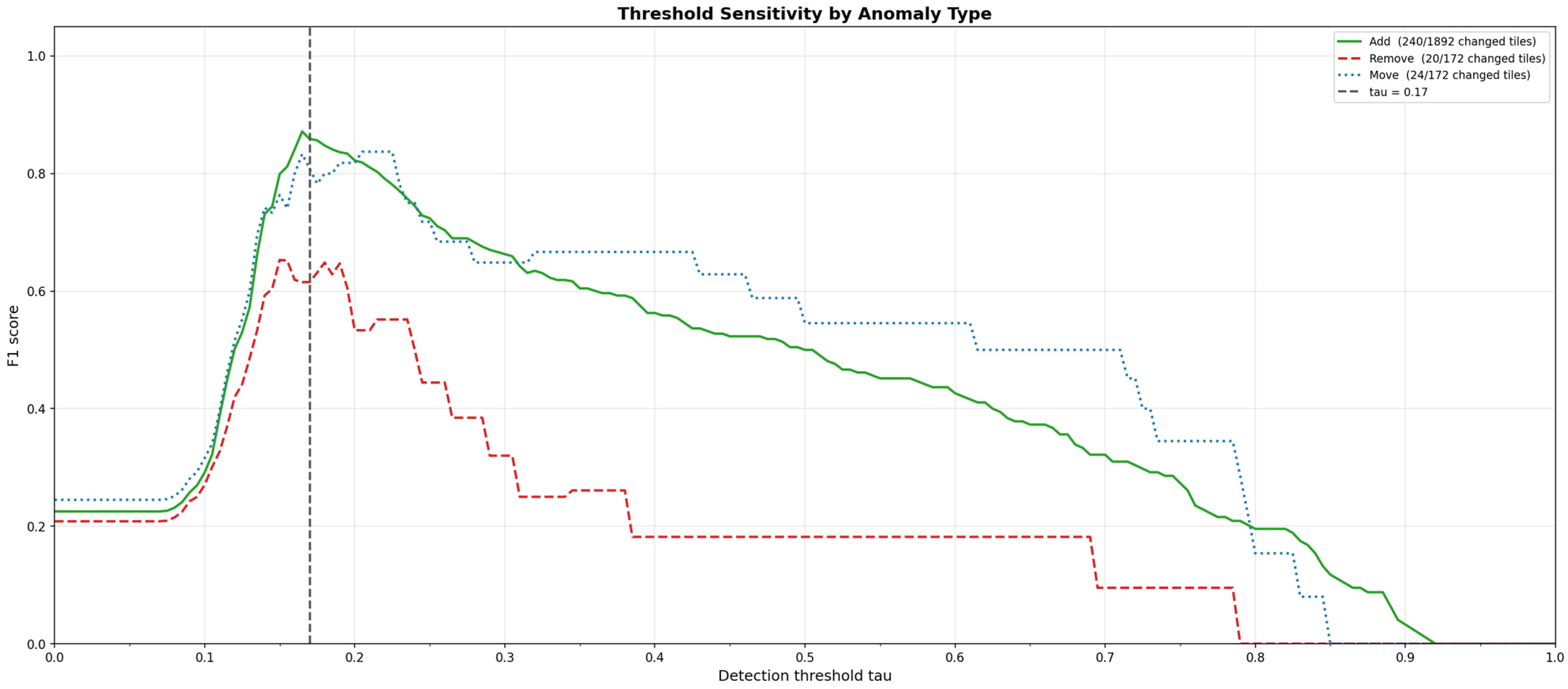
Figure 7.
Threshold sensitivity of F1-score stratified by anomaly type (add, remove, move). The add and move conditions remain stable across a wide threshold range, while remove achieves a substantially lower peak F1 (≈0.65) and exhibits greater sensitivity to threshold choice, consistent with the weaker geometric evidence produced by point removal under fixed-size patch resampling.
Figure 7.
Threshold sensitivity of F1-score stratified by anomaly type (add, remove, move). The add and move conditions remain stable across a wide threshold range, while remove achieves a substantially lower peak F1 (≈0.65) and exhibits greater sensitivity to threshold choice, consistent with the weaker geometric evidence produced by point removal under fixed-size patch resampling.
Figure 8.
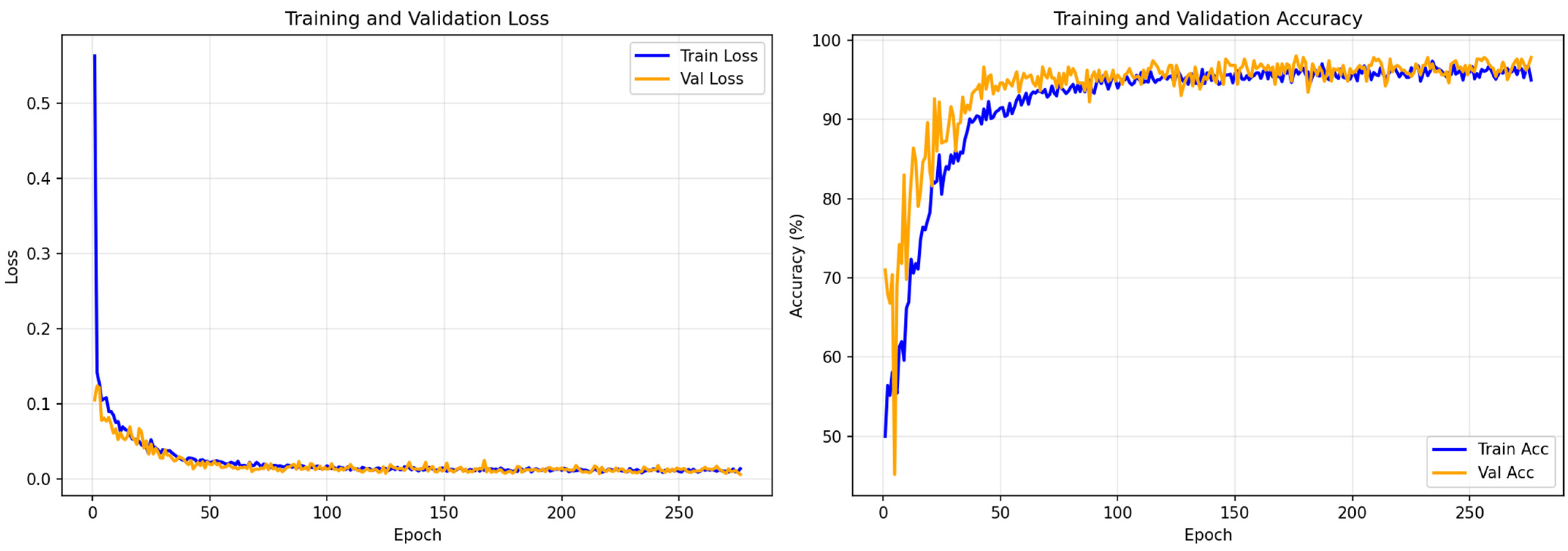
Training and validation curves showing focal loss convergence and classification accuracy over epochs, demonstrating stable optimization and absence of overfitting. Left: focal loss. Right: classification accuracy (%). Both curves converge without overfitting, indicating effective generalization from synthetic training pairs to held-out spatial regions.
Figure 8.
Training and validation curves showing focal loss convergence and classification accuracy over epochs, demonstrating stable optimization and absence of overfitting. Left: focal loss. Right: classification accuracy (%). Both curves converge without overfitting, indicating effective generalization from synthetic training pairs to held-out spatial regions.
Figure 9.
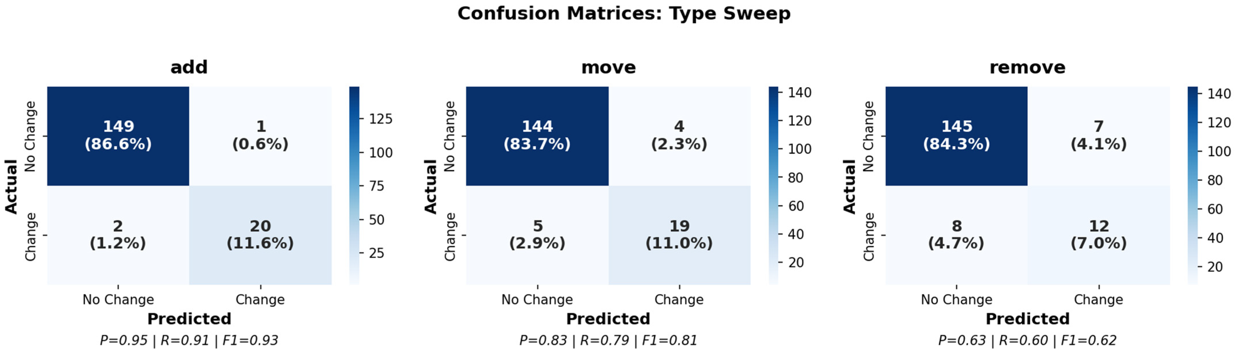
Confusion matrices for the change type series. The add operation (F1 = 0.93) substantially outperforms move (F1 = 0.81) and remove (F1 = 0.62), revealing an asymmetry in detection difficulty across change types.
Figure 9.
Confusion matrices for the change type series. The add operation (F1 = 0.93) substantially outperforms move (F1 = 0.81) and remove (F1 = 0.62), revealing an asymmetry in detection difficulty across change types.
Figure 10.
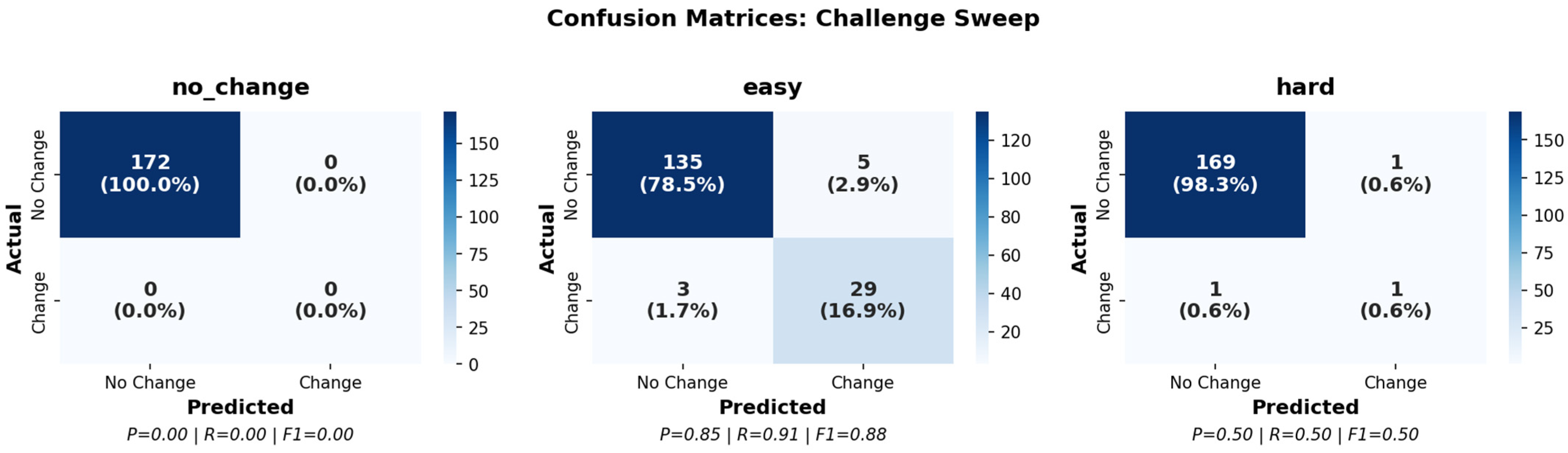
Confusion matrices for the baseline and challenge experiments. The baseline achieves zero false positives, while the easy challenge (F1 = 0.88) and hard challenge (F1 = 0.50) define the system’s operational range.
Figure 10.
Confusion matrices for the baseline and challenge experiments. The baseline achieves zero false positives, while the easy challenge (F1 = 0.88) and hard challenge (F1 = 0.50) define the system’s operational range.
Figure 11.
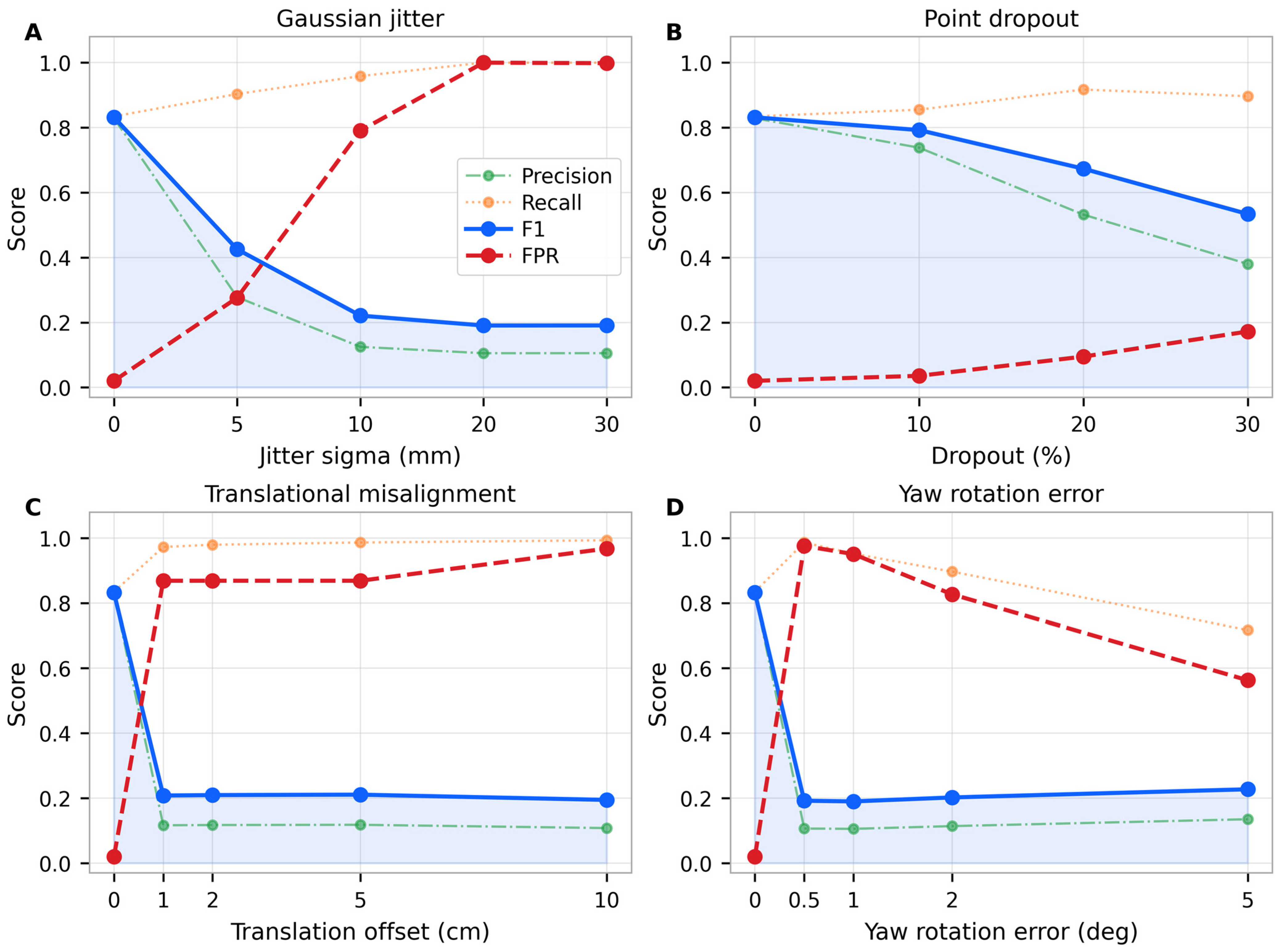
Robustness of SPICD-Net under explicit inference-time perturbations. (A) Gaussian coordinate jitter, (B) random point dropout, (C) translational misalignment, and (D) yaw rotation error. Each panel reports precision, recall, F1-score, and false positive rate (FPR) as the perturbation magnitude increases. Results are aggregated over the selected robustness-evaluation experiment subset.
Figure 11.
Robustness of SPICD-Net under explicit inference-time perturbations. (A) Gaussian coordinate jitter, (B) random point dropout, (C) translational misalignment, and (D) yaw rotation error. Each panel reports precision, recall, F1-score, and false positive rate (FPR) as the perturbation magnitude increases. Results are aggregated over the selected robustness-evaluation experiment subset.
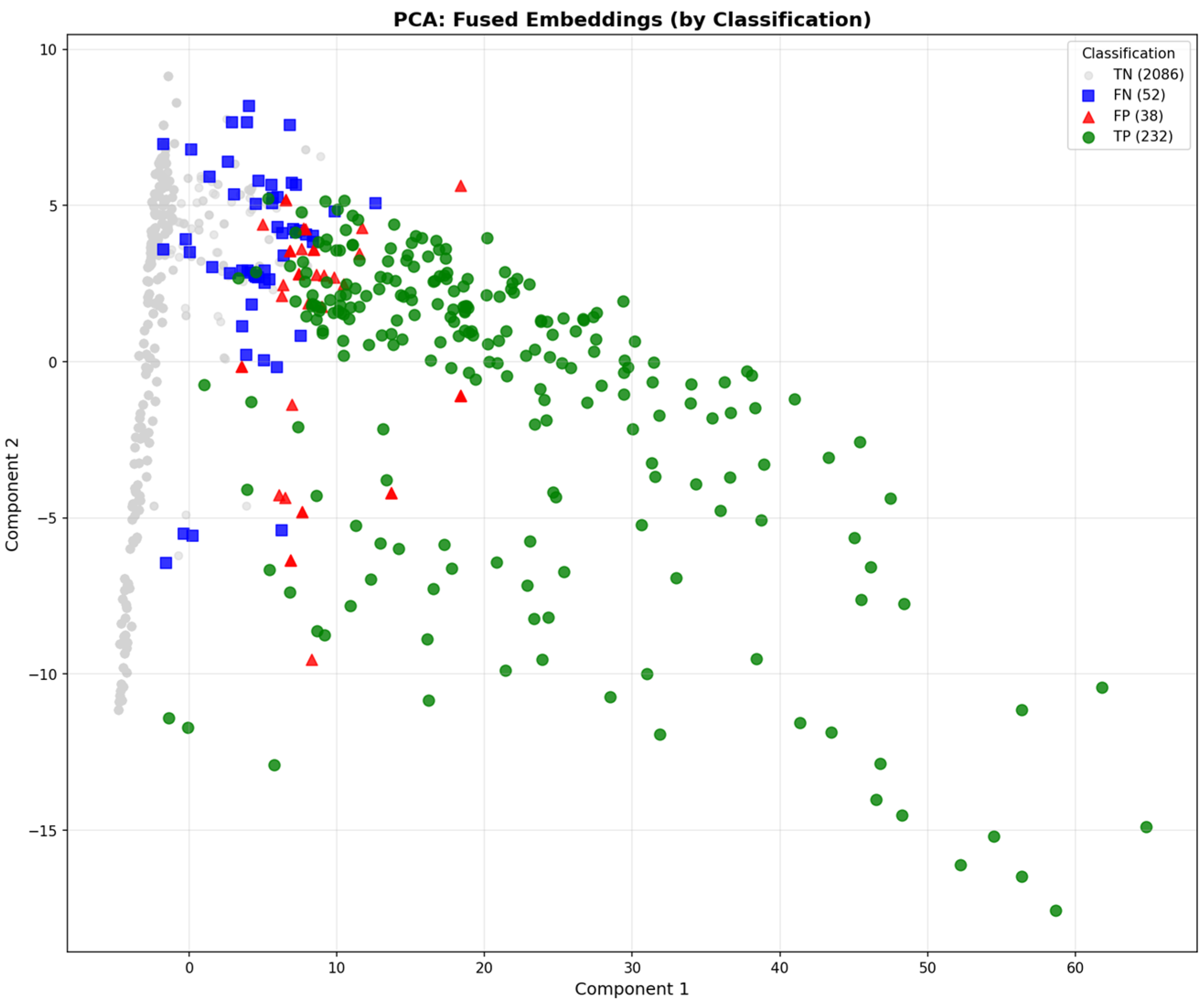
Figure 12.
PCA projection of fused embeddings colored by classification outcome. True negatives (gray) cluster at low PC1 values; true positives (green) extend to high PC1 values. FN (blue) and FP (red) occupy the boundary region, consistent with their near-threshold prediction.
Figure 12.
PCA projection of fused embeddings colored by classification outcome. True negatives (gray) cluster at low PC1 values; true positives (green) extend to high PC1 values. FN (blue) and FP (red) occupy the boundary region, consistent with their near-threshold prediction.
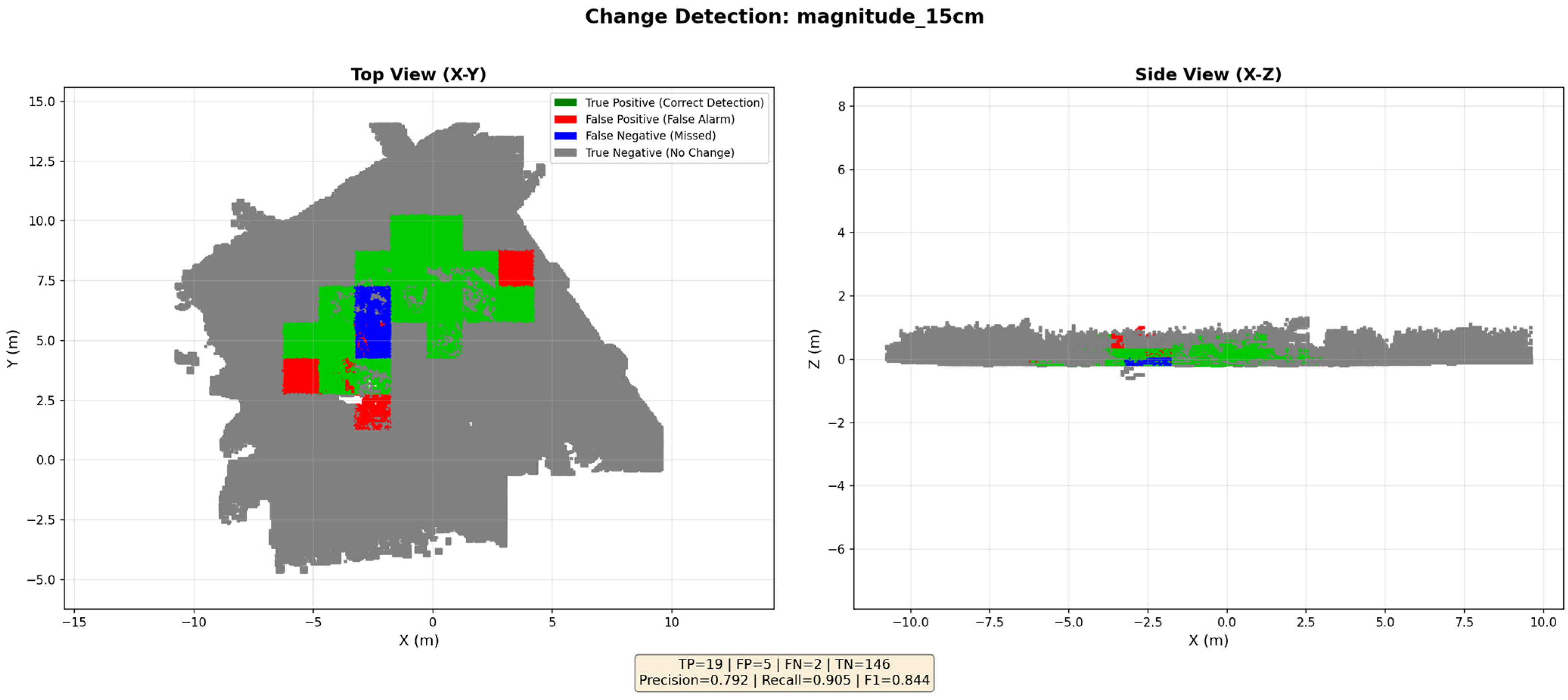
Figure 13.
Spatial change detection for the magnitude_15 cm experiment (P = 0.79, R = 0.90, F1 = 0.84). True positives (green) correctly identify the region of injected change, while false positives (red) are isolated and sparse.
Figure 13.
Spatial change detection for the magnitude_15 cm experiment (P = 0.79, R = 0.90, F1 = 0.84). True positives (green) correctly identify the region of injected change, while false positives (red) are isolated and sparse.
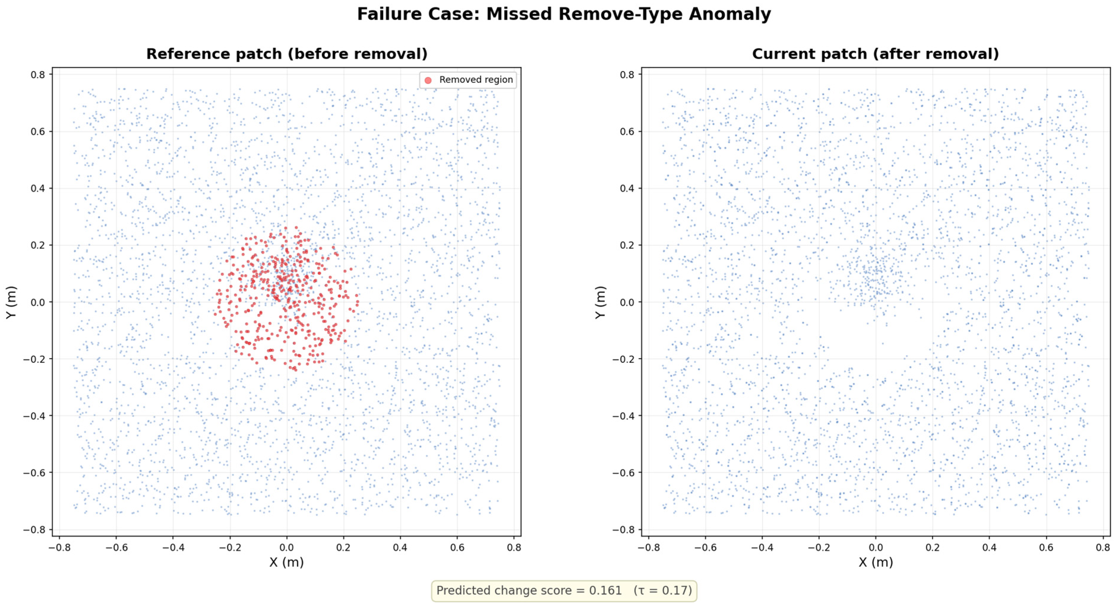
Figure 14.
Representative failure case from the type remove experiment (tile (9, 7, 0)). Left: reference patch with the removed region highlighted in red (blue points indicate retained geometry). Right: current patch after removal; the absent structure produces only a sparse geometric discrepancy under fixed-size (N = 4096) patch resampling, yielding a predicted change score of 0.161 (operating threshold τ = 0.17), resulting in a missed detection (false negative).
Figure 14.
Representative failure case from the type remove experiment (tile (9, 7, 0)). Left: reference patch with the removed region highlighted in red (blue points indicate retained geometry). Right: current patch after removal; the absent structure produces only a sparse geometric discrepancy under fixed-size (N = 4096) patch resampling, yielding a predicted change score of 0.161 (operating threshold τ = 0.17), resulting in a missed detection (false negative).
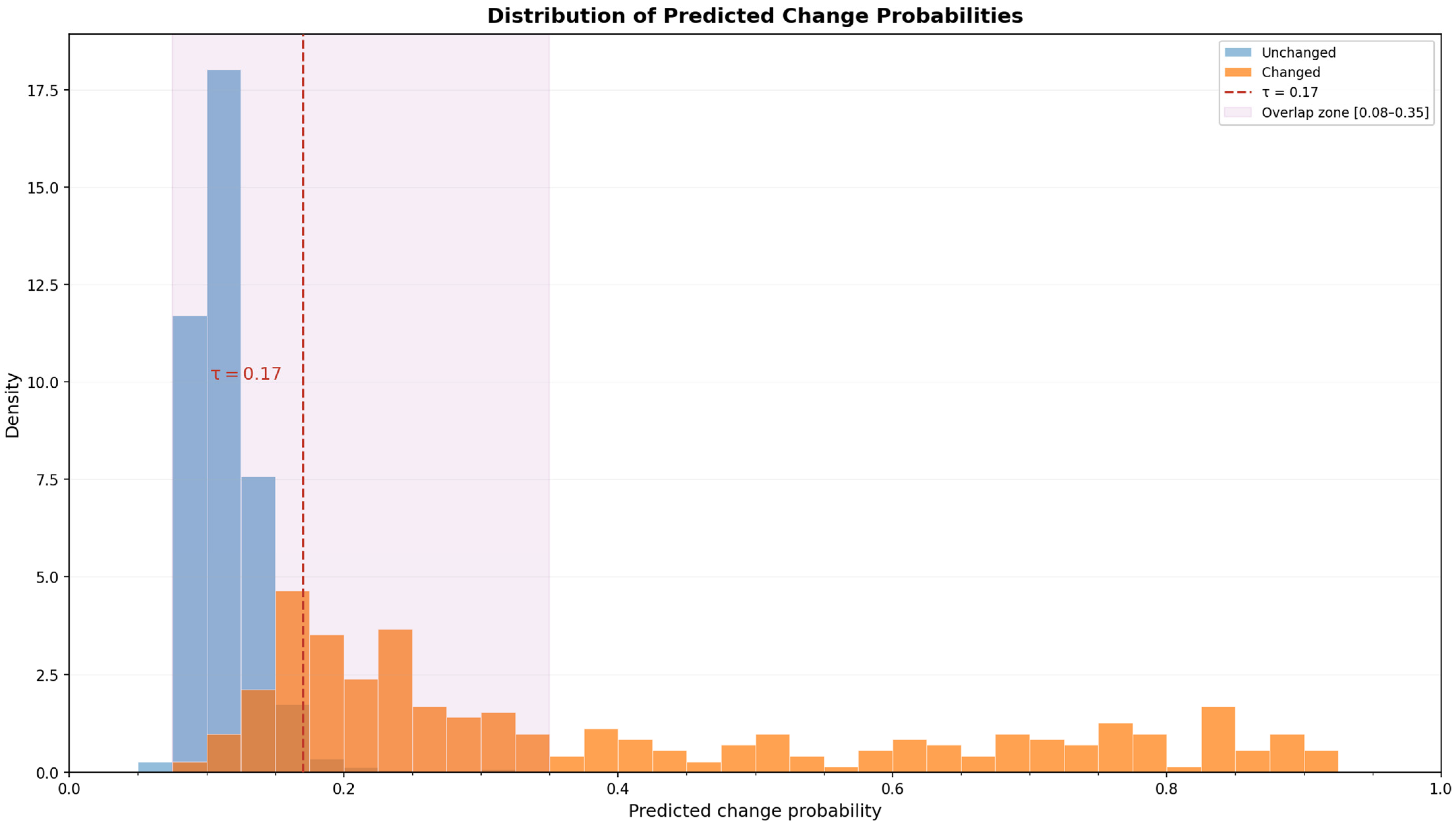
Figure 15.
Distribution of predicted change probabilities (p1) for changed tiles and unchanged tiles, pooled across all 14 simulation experiments. The dashed vertical line marks the operating threshold τ = 0.17. The prominent low-score spike in the changed-tile distribution corresponds to remove-type anomalies that receive near-zero confidence, reflecting the representational asymmetry between additive and subtractive changes under fixed-size point-cloud patch resampling.
Figure 15.
Distribution of predicted change probabilities (p1) for changed tiles and unchanged tiles, pooled across all 14 simulation experiments. The dashed vertical line marks the operating threshold τ = 0.17. The prominent low-score spike in the changed-tile distribution corresponds to remove-type anomalies that receive near-zero confidence, reflecting the representational asymmetry between additive and subtractive changes under fixed-size point-cloud patch resampling.
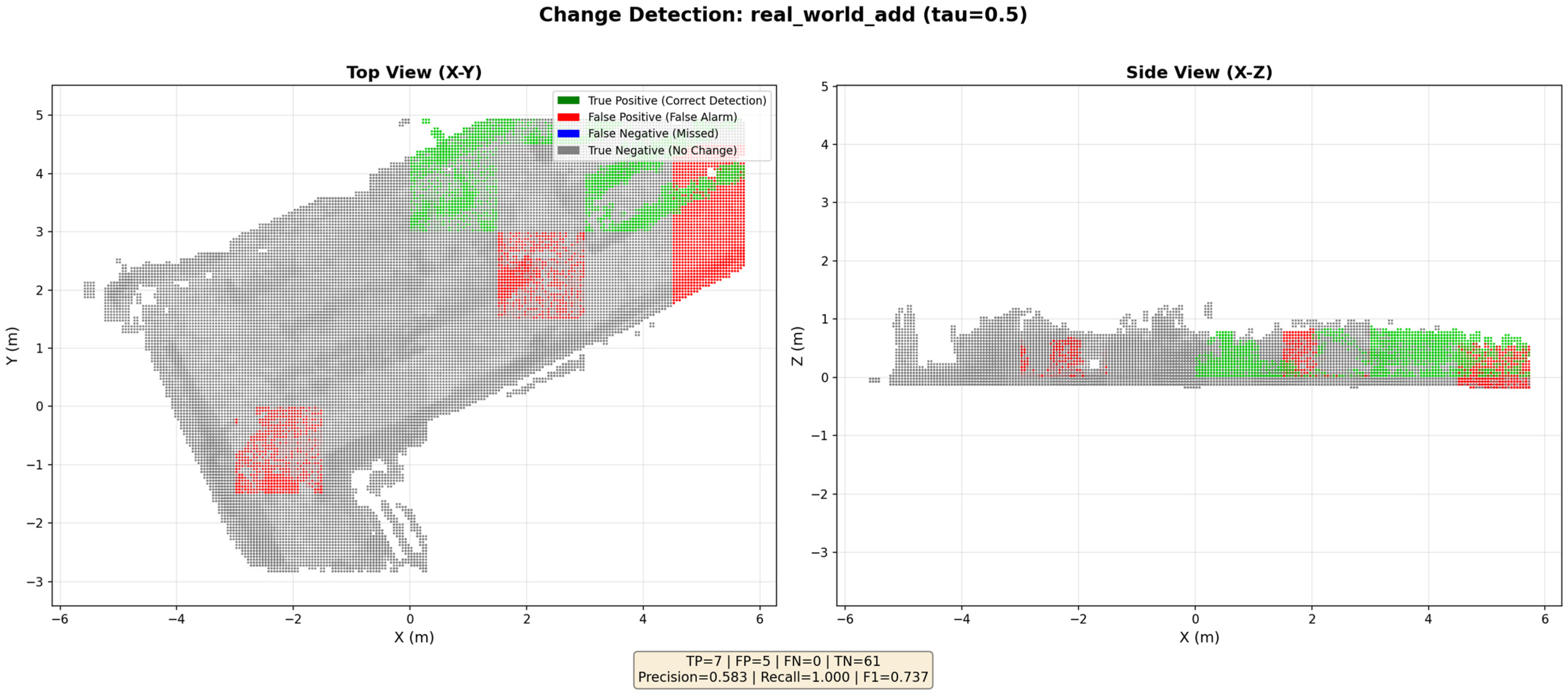
Figure 16.
Small-scale real-world validation in an unseen indoor room. The figure shows tile-level detections for an add-object case obtained from paired LiDAR scans acquired before and after inserting a box into the scene. Green denotes true positives, red false positives, blue false negatives, and gray true negatives. The model detects all annotated changed tiles (Recall = 1.00), while several false positives remain in nearby unchanged areas.
Figure 16.
Small-scale real-world validation in an unseen indoor room. The figure shows tile-level detections for an add-object case obtained from paired LiDAR scans acquired before and after inserting a box into the scene. Green denotes true positives, red false positives, blue false negatives, and gray true negatives. The model detects all annotated changed tiles (Recall = 1.00), while several false positives remain in nearby unchanged areas.
Table 1.
Registration pipeline settings used in Stage 1.
Table 1.
Registration pipeline settings used in Stage 1.
| Parameter | Value |
|---|
| ICP variant | Point-to-Plane |
| Correspondence distance threshold | 0.05 m |
| Normal estimation radius | 0.10 m |
| Normal estimation max neighbors | 30 |
| Acceptance threshold—fitness | >0.55 |
| Acceptance threshold—RMSE | <0.05 m |
| Voxel size before ICP | 0.05 m |
| Initial transformation | Identity ) |
Table 2.
Registration quality statistics for the Stage 1 map-construction pipeline.
Table 2.
Registration quality statistics for the Stage 1 map-construction pipeline.
| Statistic | Value |
|---|
| Total scans collected | 42 |
| Successful ICP registrations | 25 scans in main connected component |
| Discarded registrations | 17 scans |
| Average alignment RMSE (main component) | 2.50 ± 0.45 cm |
| Average fitness (main component) | 0.592 ± 0.089 |
Table 3.
LiDAR dataset statistics and patch sampling parameters.
Table 3.
LiDAR dataset statistics and patch sampling parameters.
| Property | Value |
|---|
| Number of raw scans | 42 |
| Sensor | Unitree 4D LiDAR L1 |
| Voxel resolution | 5 cm |
| Tile dimensions | 1.5 × 1.5 × 1.0 m |
| Points per patch (N) | 4096 |
| Minimum points per tile | 512 |
| Train/validation split | 90%/10% (spatial) |
| Training pairs per epoch | 2000 |
| Validation pairs per epoch | 500 |
Table 4.
Simulation experiment matrix. All experiments use eight tiles per modified scan unless otherwise noted.
Table 4.
Simulation experiment matrix. All experiments use eight tiles per modified scan unless otherwise noted.
| Experiment | Change Type | Magnitude (cm) | Density (%) | Modified Scans | Tiles/Scan |
|---|
| Magnitude series |
| magnitude_5 cm | add | 5 | 30 | 3 | 8 |
| magnitude_10 cm | add | 10 | 30 | 3 | 8 |
| magnitude_15 cm | add | 15 | 30 | 3 | 8 |
| magnitude_20 cm | add | 20 | 30 | 3 | 8 |
| magnitude_30 cm | add | 30 | 30 | 3 | 8 |
| Density series |
| density_10 pct | add | 15 | 10 | 3 | 8 |
| density_30 pct | add | 15 | 30 | 3 | 8 |
| density_50 pct | add | 15 | 50 | 3 | 8 |
| Type series |
| type_add | add | 15 | 35 | 3 | 8 |
| type_remove | remove | 15 | 35 | 3 | 8 |
| type_move | move | 15 | 35 | 3 | 8 |
| Challenge |
| challenge_easy | add | 30 | 50 | 4 | 8 |
| challenge_hard | add | 5 | 10 | 2 | 1 |
| Baseline |
| baseline_no_change | - | - | - | - | - |
Table 5.
Tile-level change detection results for all 14 simulation experiments at the optimized detection threshold τ = 0.17. TP: true positives; FP: false positives; FN: false negatives; TN: true negatives. The aggregated row pools confusion matrix counts across all experiments.
Table 5.
Tile-level change detection results for all 14 simulation experiments at the optimized detection threshold τ = 0.17. TP: true positives; FP: false positives; FN: false negatives; TN: true negatives. The aggregated row pools confusion matrix counts across all experiments.
| Experiment | Type | Mag. (cm) | Dens. (%) | TP | FP | FN | TN | Precision | Recall | F1 | Accuracy |
|---|
| Magnitude series |
| magnitude_5 cm | add | 5 | 30 | 18 | 1 | 6 | 147 | 0.95 | 0.75 | 0.84 | 0.96 |
| magnitude_10 cm | add | 10 | 30 | 19 | 5 | 4 | 144 | 0.79 | 0.83 | 0.81 | 0.95 |
| magnitude_15 cm | add | 15 | 30 | 19 | 5 | 2 | 146 | 0.79 | 0.90 | 0.84 | 0.96 |
| magnitude_20 cm | add | 20 | 30 | 19 | 1 | 1 | 151 | 0.95 | 0.95 | 0.95 | 0.99 |
| magnitude_30 cm | add | 30 | 30 | 20 | 3 | 4 | 145 | 0.87 | 0.83 | 0.85 | 0.96 |
| Density series |
| density_10 pct | add | 15 | 10 | 17 | 2 | 7 | 146 | 0.89 | 0.71 | 0.79 | 0.95 |
| density_30 pct | add | 15 | 30 | 21 | 2 | 3 | 146 | 0.91 | 0.88 | 0.89 | 0.97 |
| density_50 pct | add | 15 | 50 | 18 | 1 | 6 | 147 | 0.95 | 0.75 | 0.84 | 0.96 |
| Type series |
| type_add | add | 15 | 35 | 20 | 1 | 2 | 149 | 0.95 | 0.91 | 0.93 | 0.98 |
| type_remove | remove | 15 | 35 | 12 | 7 | 8 | 145 | 0.63 | 0.60 | 0.62 | 0.91 |
| type_move | move | 15 | 35 | 19 | 4 | 5 | 144 | 0.83 | 0.79 | 0.81 | 0.95 |
| Challenge |
| challenge_easy | add | 30 | 50 | 29 | 5 | 3 | 135 | 0.85 | 0.91 | 0.88 | 0.95 |
| challenge_hard | add | 5 | 10 | 1 | 1 | 1 | 169 | 0.50 | 0.50 | 0.50 | 0.99 |
| Baseline |
| baseline_no_change | - | - | - | 0 | 0 | 0 | 172 | - | - | - | 1.00 |
| Aggregated | 232 | 38 | 52 | 2086 | 0.86 | 0.82 | 0.84 | 0.96 |
Table 6.
Benchmark comparison under the unified indoor tile-level protocol. All methods were evaluated on 14 simulation experiments with the same reference tiling, current-map construction, and changed-tile ground truth. Values are micro-aggregated at the best threshold per method. M3C2-approx is a PCA-normal point-to-plane approximation, not the official CloudCompare implementation. Inference time: 172 tiles, single NVIDIA GTX 1650 (4 GB VRAM).
Table 6.
Benchmark comparison under the unified indoor tile-level protocol. All methods were evaluated on 14 simulation experiments with the same reference tiling, current-map construction, and changed-tile ground truth. Values are micro-aggregated at the best threshold per method. M3C2-approx is a PCA-normal point-to-plane approximation, not the official CloudCompare implementation. Inference time: 172 tiles, single NVIDIA GTX 1650 (4 GB VRAM).
| Method | Best τ | Precision | Recall | F1 | Accuracy | TP | FP | FN | TN | Mean Infer. (s) |
|---|
| SPICD-Net (ours) | 0.17 | 0.859 | 0.817 | 0.838 | 0.963 | 232 | 38 | 52 | 2086 | 22.4 |
| Siamese-PointNet++ | 0.20 | 0.930 | 0.845 | 0.886 | 0.974 | 240 | 18 | 44 | 2106 | 131.1 |
| Siamese-KPConv | 0.40 | 0.564 | 0.849 | 0.678 | 0.905 | 241 | 186 | 43 | 1938 | 126.1 |
| C2C | 0.01 | 0.972 | 0.366 | 0.532 | 0.924 | 104 | 3 | 180 | 2121 | 25.8 |
| M3C2-approx | 0.03 | 0.000 | 0.000 | 0.000 | 0.882 | 0 | 0 | 284 | 2124 | 23.1 |




 ,
,