1. Introduction
The rapid advancement of artificial intelligence (AI) has enabled significant progress across a wide range of domains, including autonomous systems, signal processing, healthcare, and scientific computing. However, these advances have been accompanied by a substantial increase in computational and energy demands, particularly for data-driven models deployed in large-scale data centers and high-performance computing systems [
1]. As AI workloads continue to grow, the associated power consumption and hardware costs have emerged as critical bottlenecks, motivating the development of more energy-efficient computational paradigms.
Beyond large-scale computing infrastructure, energy efficiency is an even more stringent requirement for edge and embedded applications such as wearable devices, biomedical monitoring systems, Internet-of-Things (IoT) platforms, and autonomous vehicles [
2]. In these settings, power, memory, and latency constraints limit the feasibility of conventional deep neural networks, which rely heavily on dense matrix–vector multiplications and high-precision arithmetic [
3]. Addressing these constraints requires computational models that can process temporal information efficiently while reducing hardware complexity and energy consumption.
RC has emerged as a promising framework for efficient temporal processing [
4]. In RC systems, a recurrent dynamical reservoir projects input signals into a high-dimensional state space, while only a simple readout layer is trained. By keeping the reservoir fixed and limiting training to the output layer, RC significantly reduces training complexity and computational overhead [
5]. These properties make RC particularly attractive for real-time and hardware-constrained applications [
6].
Two prominent classes of RC models are Echo State Networks (ESNs) and Liquid State Machines (LSMs) [
5]. ESNs employ continuous-valued artificial neurons with randomly initialized recurrent connections, offering efficient training through closed-form or regression-based readout solutions. In contrast, LSMs are based on spiking neural networks, where information is represented and processed through discrete spike events. The spiking dynamics of LSMs provide a biologically inspired and event-driven computational model that is naturally compatible with neuromorphic hardware platforms [
7].
To systematically evaluate the trade-offs between these two RC paradigms, this work focuses on the Mackey–Glass chaotic time-series prediction task, a widely adopted benchmark for temporal modeling and nonlinear dynamical systems [
8]. RC avoids training recurrent weights by keeping a fixed recurrent reservoir and only training a readout layer [
9]. The Mackey–Glass time series exhibits long-term temporal dependencies and chaotic behavior, making it a standard benchmark for assessing memory capacity and generalization in recurrent models.
In this paper, we present a comprehensive experimental comparison between ESNs and LSMs on two public time-series prediction tasks: the Mackey–Glass and NARMA10 datasets, with particular emphasis on scalability, overfitting behavior, and robustness to reduced numerical error precision. We evaluate model performance across varying reservoir sizes and quantization levels, analyzing both training and testing error to assess generalization. Our results show that while ESNs achieve lower prediction error with relatively small reservoirs, their performance saturates early and exhibits signs of overfitting as model size increases. In contrast, LSMs demonstrate improved scalability, greater resistance to overfitting, and strong robustness under aggressive reservoir quantization, highlighting their potential for energy-efficient and neuromorphic computing applications.
In addition to algorithmic performance, this work explicitly considers hardware implications arising from reduced numerical error precision in reservoir computation. By analyzing the impact of reservoir quantization on both ESN and LSM performance, we provide insight into how architectural choices influence memory usage, arithmetic complexity, and robustness in hardware implementations, supporting the broader goal of hardware–software co-design for practical deployment.
2. Background
2.1. Neural Network for Artificial Intelligence
Artificial Neural Networks (ANNs), inspired by the neuron connections of the human brain, have become a cornerstone of modern artificial intelligence. These models are typically organized in several layers where each layer contains a number of nodes, i.e., neurons, and are trained to perform specific tasks by adjusting the strengths, or weights, which exist between neurons of two consecutive layers [
10]. A common architecture is the feed-forward neural network (FNN), where information flows in one direction from an input layer, through one or more hidden layers, to an output layer. Although FNNs are powerful for static pattern recognition, they are inherently limited in processing sequential or temporal data, as they lack an internal memory of past events [
11].
To address this issue, recurrent neural networks (RNNs) were developed. RNNs introduce recurrent connections that form an internal state or memory which allows them to process sequences of data of arbitrary lengths [
11]. This ability makes them theoretically well suited for tasks such as speech recognition, natural language processing, and time-series analysis. However, training traditional RNNs using standard backpropagation-through-time (BPTT) is notoriously difficult [
5]. This method is computationally expensive and suffers from the vanishing and exploding gradients problem, where the error signals either shrink to zero or grow uncontrollably as they propagate through many time steps, making it difficult to learn long-term dependencies [
10]. These challenges have historically limited the practical application of RNNs, reserving state-of-the-art performance for experts in the field [
5,
11].
2.2. Reservoir Computing (RC)
RC emerged as an example to harness the power of RNNs while bypassing their difficult training procedures [
11]. The core principle of RC is to decouple the recurrent part of the network from the trained output layer [
12]. An RC system consists of a “reservoir”, i.e., a large, fixed, and randomly connected set of neurons in the hidden layer and a “trainable” readout layer [
9]. The input neuron sends the data signal to the complex dynamics of the reservoir, which acts as a nonlinear temporal filter. This process maps the low-dimensional input signal into a high-dimensional feature space, where the information becomes much easier to decode [
11]. A crucial distinction of the RC hidden layer is that the connections within the reservoir are not trained; they are initialized randomly and remain fixed. The only part of the system that undergoes training is the readout layer, which learns to map the reservoir’s dynamic states to the desired output, typically through a simple and efficient method like linear regression.
This approach offers significant advantages, including drastically faster training times, lower computational complexity, and a natural suitability for hardware implementation [
6]. Two primary models dominate the RC field: ESNs [
12], which typically use analog, rate-based neurons, and LSMs [
5], which are based on more biologically realistic spiking neurons. Despite their different neuron models, both architectures share the fundamental principle of using a fixed, dynamic reservoir to transform inputs for simplified and efficient learning at the output stage [
11].
2.3. Recent Developments of RC
Recent advancements in RC have been closely tied to the growth of neuromorphic computing [
1], which seeks to develop hardware that emulates the brain’s energy efficiency and parallel processing capabilities [
1]. The inherent hardware-friendliness of RC makes it well suited for different temporal applications [
3]. Significant progress in emerging physical substrates has enabled the creation of diverse and powerful RC architectures. These include devices based on memristors [
1], photonics [
2], spintronics [
3], and mixed-signal CMOS [
4], which can implement RC with extremely low power consumption, making them suitable for real-time embedded intelligence [
13]. Hardware platforms like Intel’s Loihi neuromorphic research chip have demonstrated the practical feasibility of deploying large-scale spiking reservoir systems in practice [
3]. This convergence of RC principles with novel neuromorphic hardware is paving the way for a new generation of low-power, event-driven, and intelligent systems capable of processing complex, real-world temporal data [
3,
9,
11,
14,
15].
Ongoing research developments in RC, particularly in the genre of neuromorphic computing, have demonstrated growing momentum toward physical and efficient implementations. Hardware platforms like Intel’s Loihi chip have shown the feasibility of spiking RC in practice [
5]. Recent work has explored hardware-friendly RC systems spanning memristive, photonic, and spintronic substrates, as well as spiking reservoir implementations on neuromorphic processors. These developments suggest that RC can provide competitive temporal processing performance while reducing training complexity and enabling efficient deployment on low-power hardware platforms [
3,
6,
9,
11,
12,
13,
14,
15].
RC has been proven highly effective across a broad range of applications, especially where temporal or sequential data is involved. In autonomous systems, RC has been combined with temporal-aware machine learning to enhance driving behavior analysis [
14], enabling systems to better recognize and respond to time-sensitive patterns. RC models also excel in spectrum sensing [
14], robotics [
1], time-series forecasting [
8] and speech recognition domains [
15] that require real-time processing with low computational overhead. The RC framework’s ability to process time-dependent data without extensive backpropagation training makes it particularly suitable for energy-constrained environments and edge AI applications. The flexibility to implement RC in both digital and analog hardware further broadens its utility in scenarios where speed, latency, and power are critical constraints.
2.4. Challenges of RC
Despite all the mentioned advances and diverse applications, challenges persist in scaling and stabilizing RC for practical deployment. Physical implementations often suffer from hardware variability, limited control over reservoir dynamics, and non-ideal reproducibility [
6,
9,
15]. Once deployed, tuning hyperparameters or modifying architecture is typically difficult, especially in analog systems. The lack of standardized benchmarks for neuromorphic RC also complicates performance evaluation across platforms [
6,
7]. Furthermore, real-world deployment of RC demands integration of adaptive and online learning mechanisms, such as biologically inspired synaptic plasticity, which remains largely underexplored in hardware systems [
8,
15]. Addressing these challenges will be key to advancing RC from a promising research tool to a mainstream solution in neuromorphic and embedded AI systems.
3. Development of RC
The contribution of this work is not the proposal of a novel reservoir architecture, but a rigorous, hardware-aware benchmarking study of the state-of-the-art RC frameworks evaluated under identical experimental conditions. By systematically analyzing the impact of reservoir size and weight precision on prediction accuracy and generalization, this study provides insights that are directly relevant to efficient neuromorphic hardware–software co-design development for time-series applications. This section discusses the state-of-the-art algorithmic design of two fundamental RC architectures: ESN and LSM.
3.1. Theory Development of RC
RC emerged as a framework for temporal information processing that avoids the instability and computational burden of training fully recurrent networks. Its defining principle is the separation of a fixed, nonlinear dynamical reservoir from a simple, trainable readout layer. Two canonical models dominate the RC landscape: the ESN, which employs rate-based neurons and discrete-time dynamics, and the LSM, which uses biologically inspired spiking neurons and continuous-time membrane dynamics. This section develops the theoretical foundations of both models, establishing their computational properties, mathematical formulations, and relevance for neuromorphic implementation [
5,
8].
3.2. ESN
3.2.1. Theory Derivative of ESN
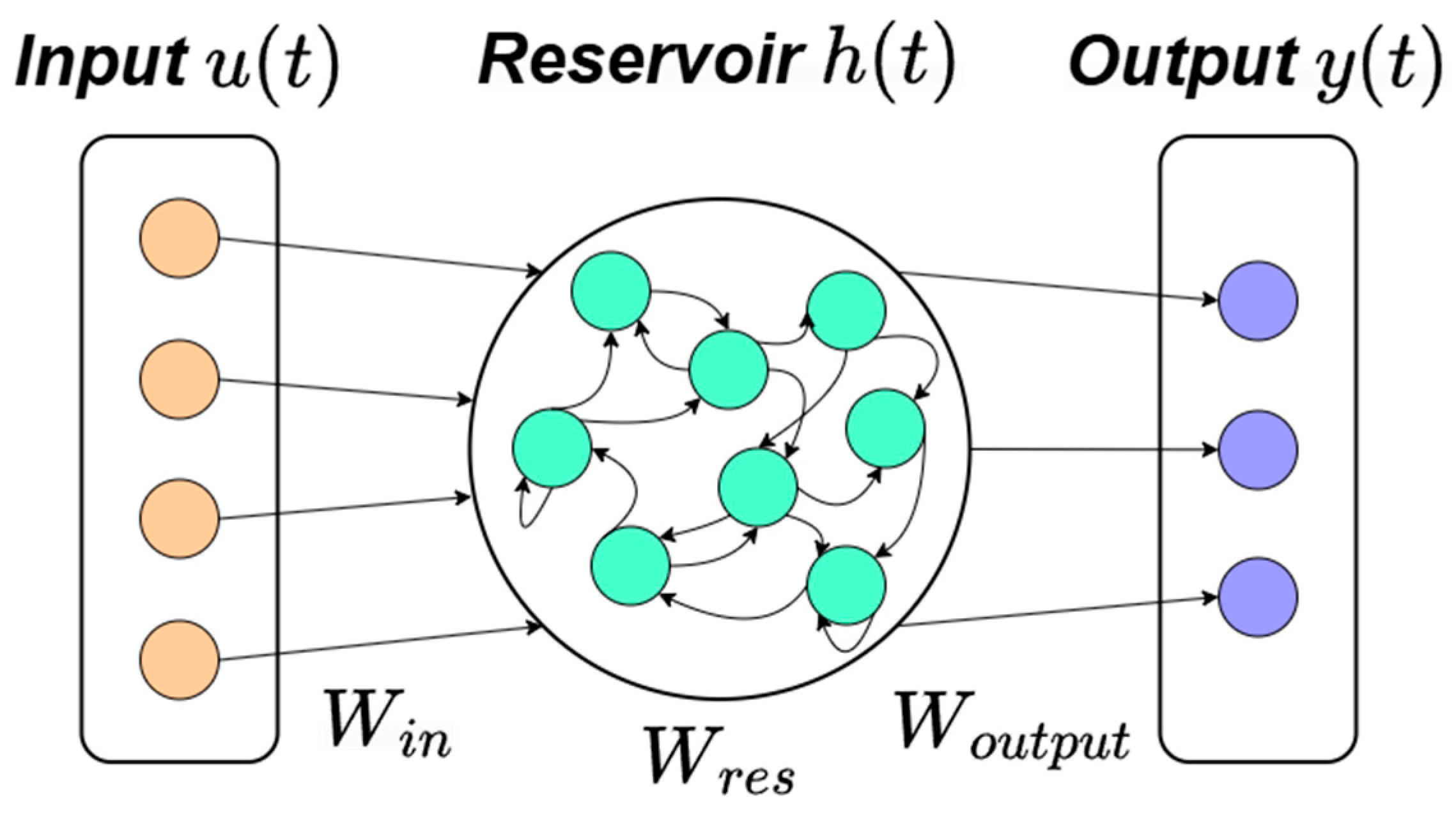
The ESN as illustrated in
Figure 1, represents the canonical artificial-neuron formulation of RC. It consists of a fixed, recurrent reservoir whose internal weights are initialized randomly and remain unchanged throughout training, while only the readout weights are adapted. This design dramatically simplifies learning and avoids the instability issues that arise in fully trained recurrent neural networks. Formally, the reservoir state evolves according to the discrete-time update equation in Equation (1):
where
denotes the reservoir state at time
,
is the input signal,
is the input weight matrix,
is the recurrent reservoir weight matrix,
is an optional feedback matrix, and
is typically a tanh activation.
A fundamental requirement for ESNs is the echo state property (ESP), which ensures that the influence of initial conditions diminishes over time, making the reservoir state determined solely by the input history. A sufficient practical condition for the ESP is to scale the reservoir such that its spectral radius satisfies
, although tasks requiring long temporal memory sometimes benefit from values slightly above unity to place the reservoir near the “edge of chaos” [
9,
12].
Key hyperparameters governing ESN behavior include the reservoir size
, input scaling, reservoir sparsity, and spectral radius. These parameters shape the richness and stability of internal dynamics and strongly affect the model’s ability to capture long-range temporal dependencies. Once the reservoir states are collected, the output is computed through a linear readout of the form
with
obtained by ridge regression
where
is the matrix of collected reservoir states,
is the target output matrix, and
is the regularization parameter [
9]. This closed-form update avoids the need for backpropagation-through-time, making ESNs both computationally efficient and hardware-friendly.
3.2.2. Neuromorphic Computing of ESN
The structure of ESNs aligns naturally with neuromorphic and hardware-accelerated computing models. Because the reservoir is fixed, ESNs avoid continuous weight updates during training, which significantly reduces hardware complexity. ESN and RC approaches have been explored for low-power and hardware-friendly deployment, including FPGA-based acceleration for wireless communications tasks such as OFDM symbol detection [
2,
16].
In hardware, the reservoir dynamics can be implemented using lightweight multiply–accumulate blocks, or even analog charge-based circuits, while the readout—being linear—can be trained offline and deployed as a low-cost, feed-forward module. Such implementations enable high-throughput, low-latency temporal inference while consuming substantially less power than conventional deep learning models. These properties position ESNs as a strong candidate for edge-intelligent systems operating under the stringent latency and power constraints of Next-G wireless communication.
3.3. LSM
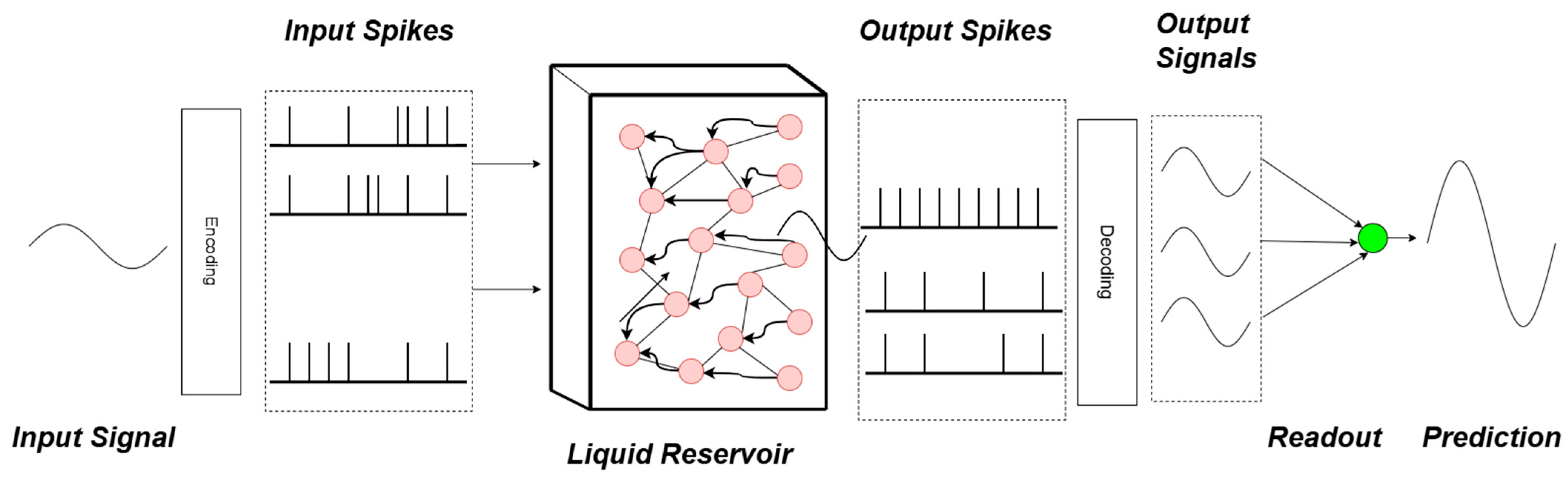
LSMs (shown in
Figure 2) generalize the RC paradigm into the domain of spiking neural networks, using biologically inspired neuron models and continuous-time membrane dynamics rather than analog activations. Whereas ESNs rely on discrete-time rate neurons, LSMs operate on event-based spike interactions, allowing them to encode fine temporal detail and enabling high degrees of sparsity and computational efficiency. The theoretical foundations of LSMs were established by Maass et al. [
14], who demonstrated that spiking reservoirs satisfy universal computation properties when equipped with separation and fading-memory dynamics. As in ESNs, the reservoir (liquid) is fixed after initialization, and only the readout layer is trained. The resulting high-dimensional temporal representation is particularly effective for chaotic time-series modeling, real-time edge inference, and neuromorphic deployment. Quantized variants have further shown that LSMs retain performance even under reduced bit precision, strengthening their suitability for low-power hardware [
9,
17].
3.3.1. Theory Derivative of LSM
An LSM consists of an encoding stage that converts the continuous input signal
into spike trains, a recurrent spiking reservoir whose dynamics evolve through membrane and synaptic interactions, and a linear readout layer that maps reservoir activity into the final output. The computational capability of the liquid depends on two key properties introduced by Maass et al. [
14]: the separation property, which requires that different inputs generate distinguishable liquid trajectories, and the fading-memory property, which ensures that remote past inputs gradually lose influence over the reservoir state.
The reservoir is typically composed of leaky integrate-and-fire (LIF) neurons. For neuron
, the membrane potential is governed by Equation (4):
where
is the membrane time constant,
is the resting potential,
is the membrane resistance, and
denotes the total synaptic input current [
11]. A spike is emitted when
after which the neuron may enter a refractory period.
The synaptic current aggregates contributions from all presynaptic neurons according to
where
is the synaptic weight and
is a postsynaptic kernel, typically modeled as
with synaptic time constant
.
Because the liquid only processes spikes, the analog input must be encoded into spike trains. In rate encoding, spikes are generated according to a Poisson process with instantaneous rate
whereas temporal encoding emits spikes only when the input signal changes by more than a threshold, producing separate streams for positive and negative variations. These encoding mechanisms follow the formulation described in the quantized LSM framework [
17].
For training, the reservoir’s spiking output must be transformed into a continuous representation. A common approach is Gaussian smoothing of each neuron’s spike train:
where
is the
-th spike of neuron
and
controls the smoothing window [
17]. After decoding, the LSM produces a continuous reservoir state vector
that summarizes recent spiking activity. The readout is implemented as a single linear regressor,
where
are the only trainable parameters. Unlike ESNs (which often use a closed-form ridge solution), we optimize the LSM readout by minimizing the mean squared error over the training sequence in Equation (11)
using the Adam optimizer with mini-batch updates. This loss-based training setup follows the quantized LSM evaluation pipeline, where predictive accuracy is reported via MSE-based readout performance [
17].
3.3.2. Neuromorphic Computing of LSM
Neuromorphic hardware is especially well aligned with LSM computation due to its sparse, event-driven nature. Unlike ESNs, which require continuous-valued multiply–accumulate operations, LSM reservoirs operate through membrane integration, threshold crossings, and spike-driven synaptic updates, with these operations efficiently implemented in mixed-signal CMOS neurons, memristive crossbars, and digital neuromorphic processors such as Intel Loihi [
3,
7,
9]. Quantized LSM implementations further demonstrate that membrane potentials, thresholds, and synaptic weights may be stored using as few as 2–3 bits while preserving predictive performance. Voshol [
17] shows that 3-bit LSMs maintain accuracy comparable to 16-bit implementations while reducing computational activity by over 50%, supporting their use in resource-constrained edge environments.
4. Experimentation and Results
This section evaluates the performance of ESNs and LSMs on the Mackey–Glass chaotic time-series prediction task. The experiments are designed to analyze predictive accuracy, scalability with respect to reservoir size, and robustness to reduce error precision. All results are reported using mean squared error (MSE) and mean absolute error (MAE). For the ESN, the readout is trained by ridge regression with fixed reservoir dynamics. For the LSM, the spiking reservoir is fixed after initialization, and the readout is optimized to minimize MSE using the Adam optimizer.
4.1. Hyperparameter Selection and Fair Comparison
To ensure a fair comparison between ESN and LSM architectures, the dataset split, prediction range, and evaluation metrics were kept consistent across all experiments. Both models performed one-step-ahead prediction on the same Mackey–Glass segment, and preprocessing was applied consistently within each model using parameters computed on the training split and applied to the test split. Random seeds were fixed to ensure reproducibility across reservoir initializations.
Hyperparameters were selected via manual hyperparameter tuning through exhaustive experiments. For each model family, we conducted controlled sweeps over performance-critical parameters (summarized in
Table 1) while keeping all other settings fixed. For each reservoir size and quantization level, we selected the configuration based on performance trends observed across exhaustive experiments under identical train/test splits and reported final MSE on the test set using the selected configuration.
To maintain fairness, we used the same prediction range, data split, preprocessing, and evaluation metric for both models. Hyperparameter search effort was comparable across ESN and LSM, and selection was based on performance trends observed across exhaustive experiments under identical train/test splits.
It can be noted from
Table 1 that ESN uses only 1 epoch for training, whereas LSM requires iterative training. This is due to the training procedure of the readout layer. In terms of updated weight parameter calculation for ESN, a closed ridge regression is used that uses a pseudo-inverse operation, as mentioned in Equation (3). Such an operation can analytically compute the optimal weights of the readout layer by collecting reservoir states and target outputs, which eliminates the need for multiple iterations for tuning. This contrasts with LSMs, which employ adaptive training requiring repeated exposure to data for effective learning. Using each model’s standard training approach ensures optimal performance and maintains methodological rigor in comparison.
4.2. Dataset Description
To evaluate the ESN and LSM architectures under consistent preprocessing, target signals, and fixed random seeds, we use the Mackey–Glass time-delay dynamical system, a standard benchmark for testing nonlinear time-series prediction models. The continuous-time Mackey–Glass system is defined as
with commonly used parameters
,
, and
and a time delay of
. The resulting trajectory exhibits stable chaotic dynamics, making it an ideal test for temporal memory and nonlinear modeling capacity [
5,
8].
To evaluate ESN and LSM architectures under consistent preprocessing and target signals, we use the Mackey–Glass time series from the Mackey–Glass Anomaly Benchmark (MGAB) repository [
18]. MGAB provides Mackey–Glass trajectories generated from the Mackey–Glass time-delay differential equation originally introduced in [
19]. In this work, we use the MGAB time-series values (the value column) as a chaotic prediction benchmark and do not use the anomaly labels.
For the segment used in our experiments (6000 samples), the Mackey–Glass values have a minimum of 0.2682, maximum of 1.6472, mean of 0.9605, and variance of 0.1014. We apply normalization prior to training using parameters computed on the training split and applied consistently to the test split.
We use a consistent split for both ESN and LSM experiments, 5000 training samples and 1000 testing samples, and perform one-step-ahead prediction throughout.
To ensure fair comparison, all experiments use fixed random seeds and identical target signals. Model performance is evaluated using both training and testing MSE to assess fitting capacity and generalization behavior.
4.3. ESN Experimental Results
The ESN is evaluated across reservoir sizes of neurons. For each configuration, the reservoir weights are initialized randomly and scaled to satisfy the echo state property, while the readout layer is trained using ridge regression. In addition to the full-precision baseline, the ESN reservoir weights are quantized to 2-bit, 3-bit, 6-bit, and 16-bit precision to evaluate sensitivity to numerical error precision.
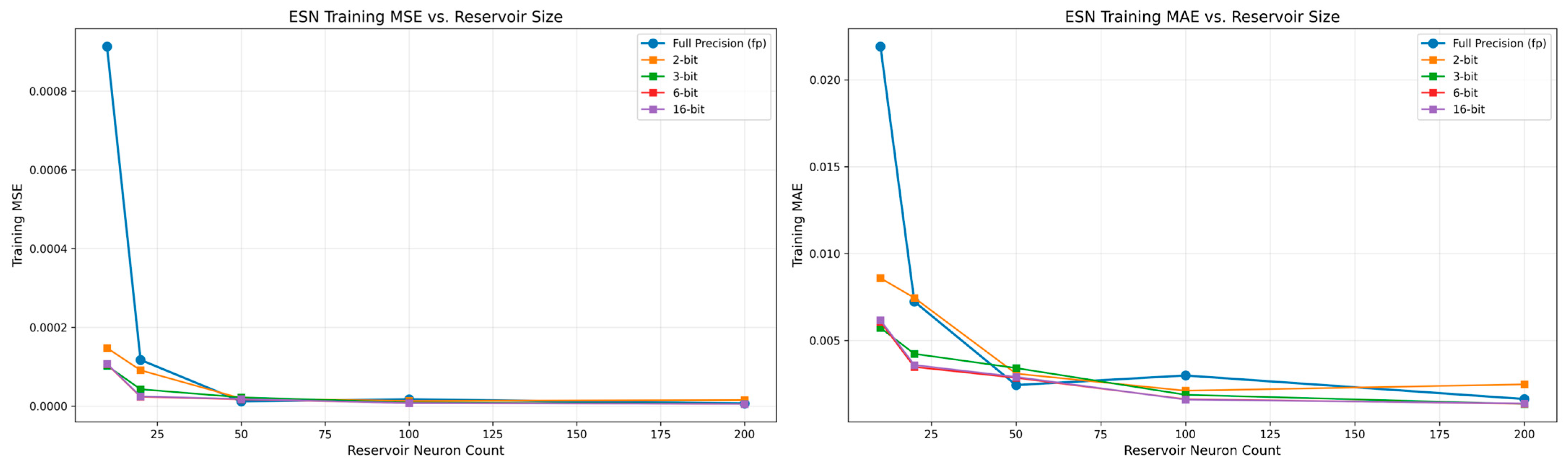
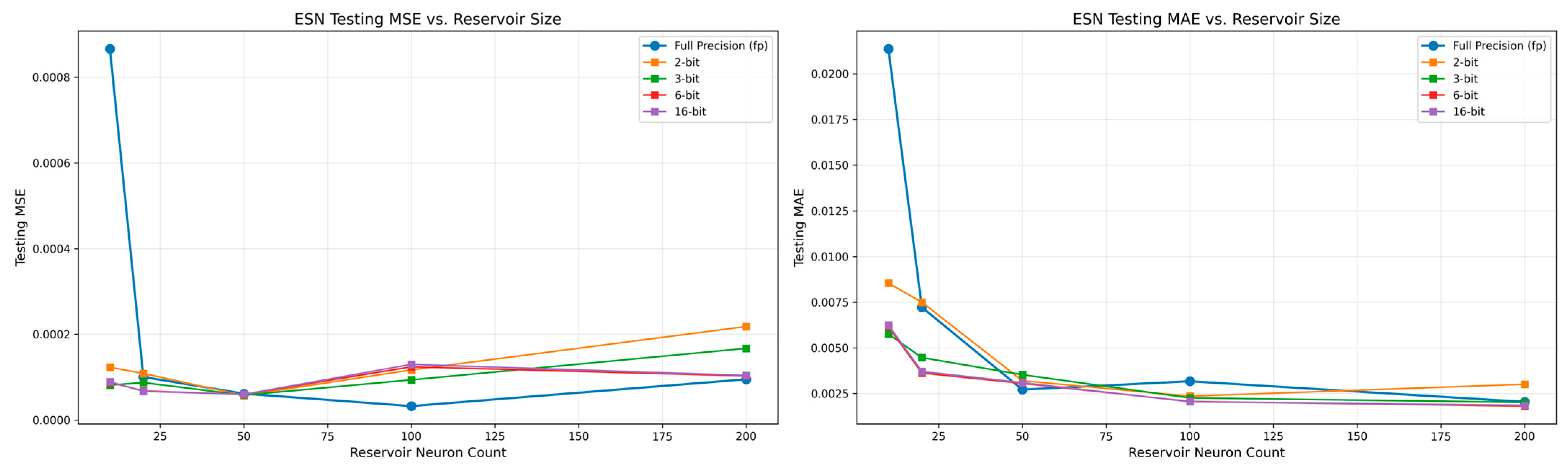
Across all configurations, both training MSE and MAE decrease rapidly as reservoir size increases, with diminishing improvements beyond approximately 50 neurons. On the test set evaluations, more distinctions can be inferred from the MSE compared to the MAE graph. The MSE plot reveals that the ESN performance on unseen data is more prone to reduced accuracy at lower reservoir bit widths, as evidenced by the 2-bit reservoir ESN, whose test MSE begins to increase at significantly smaller reservoir sizes compared to ESNs with higher bit precisions. Although quantizing the reservoir weights (2-bit, 3-bit, 6-bit, 16-bit) introduces only minor variation in training, the testing MSE/MAE perspective suggests that ESNs are more likely to result in less accurate performance on unseen data over reduced reservoir bit-precision size.
Regularization Tuning
Because the ESN readout is trained using ridge regression, we explicitly sweep the ridge regularization coefficient
(implemented as alpha in the Ridge regressor) to examine whether stronger regularization can mitigate the observed saturation/mild overfitting trend at larger reservoir sizes. Using the same Mackey–Glass split and the same ESN configuration as the main experiments, we evaluate multiple
values for a representative large reservoir size (
N = 200) under both full precision and low-bit quantization (2-bit).
Table 2 reports the resulting test MSE across
. The best-performing β is selected and used as the default regularization setting in the ESN experiments.
As shown in
Table 2, performance is highly sensitive to
. The lowest test MSE occurs at
for both full precision and 2-bit quantization, while both weaker and stronger regulation degrade performance. We therefore use
as the default ESN regularization setting in subsequent ESN experiments.
4.4. LSM Experimental Results
The LSM is evaluated using reservoir (liquid) sizes of neurons. The input signal is converted into three spike train channels using a combination of rate-based and temporal spike encoding (positive and negative threshold-based spike trains). The spiking reservoir consists of leaky integrate-and-fire neurons with sparse recurrent connectivity. Spike outputs are transformed into continuous-valued state representations using Gaussian decoding prior to readout training.
For each liquid size, experiments are conducted using reservoir state quantization at 2-bit, 3-bit, 6-bit, and 16-bit precision.
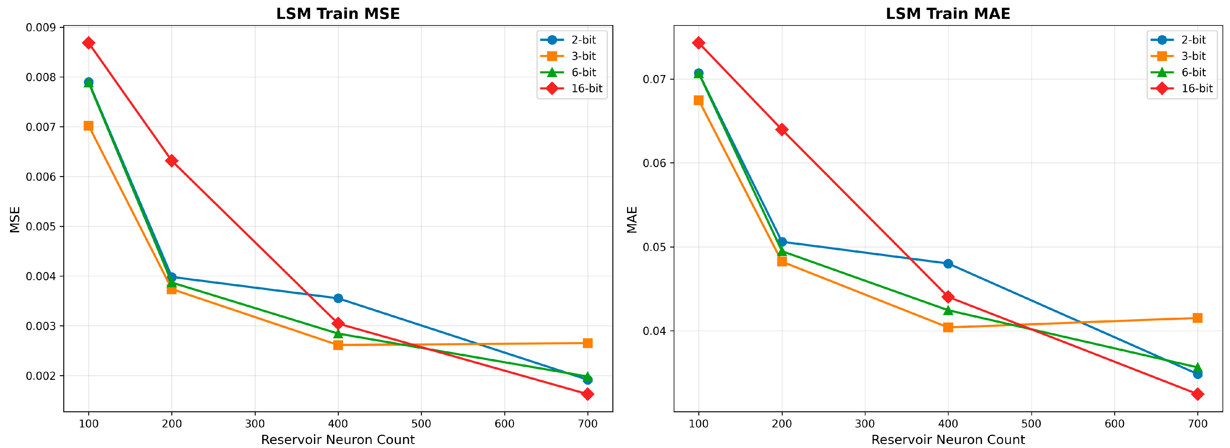
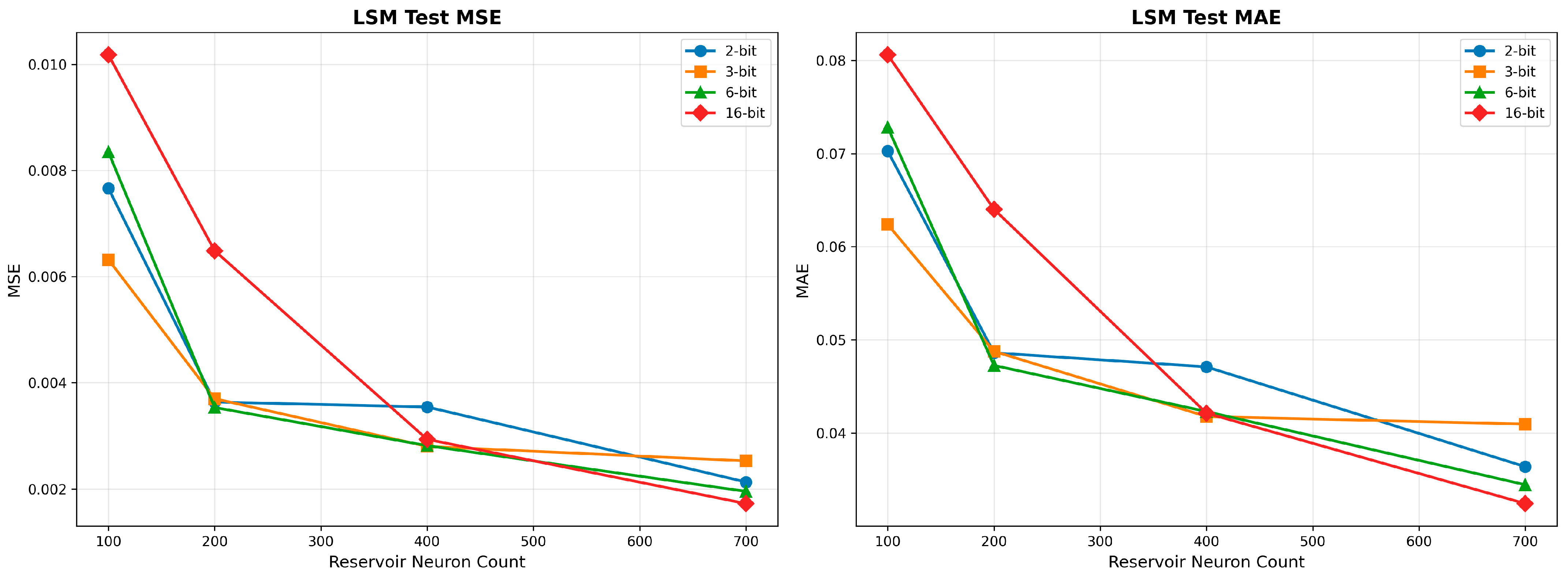
Training and testing MSE and MAE decrease steadily as the liquid size increases across all quantization levels. As the reservoir neuron count increases, higher-precision bit-width reservoirs consistently achieve slightly lower MSE compared to their lower-precision counterparts. In contrast to the ESN, a key characteristic of the LSM is that the testing MSE continues to decrease with increasing reservoir size regardless of the quantization level. Overall, the LSM shows consistent improvement in both MSE/MAE with increased liquid size, supporting its scalability under reduced precision.
Overfitting and Generalization Behavior
Overfitting is indicated when training error continues to decrease while testing error stagnates or increases, reflecting reduced predictive performance on unseen data.
In the case of the ESN,
Figure 3 and
Figure 4 show that increasing the reservoir size rapidly reduces training errors in both MSE and MAE. However, beyond approximately 50 to 100 neurons, the testing MSE and MAE exhibit limited improvement and in some configurations begin to increase. This divergence between training and testing performance indicates the onset of overfitting, where the ESN increasingly memorizes the training sequence without corresponding gains in generalization.
In contrast, the LSM demonstrates a different scaling behavior. As shown in
Figure 5 and
Figure 6, both training and testing error decrease consistently in terms of MSE and MAE as the liquid size increases from 100 to 700 neurons. No pronounced divergence between training and testing MSE/MAE is observed within the evaluated range, suggesting that the LSM is more resistant to overfitting under increasing model capacity.
These observations highlight a key distinction between ESN and LSM architectures: while ESNs achieve low error with relatively small reservoirs, their generalization performance saturates early, whereas LSMs benefit more directly from increased reservoir size while maintaining stable generalization. This difference is particularly relevant for hardware-constrained and neuromorphic systems, where model robustness and scalability are critical considerations.
4.5. ESN-LSM Comparative Analysis
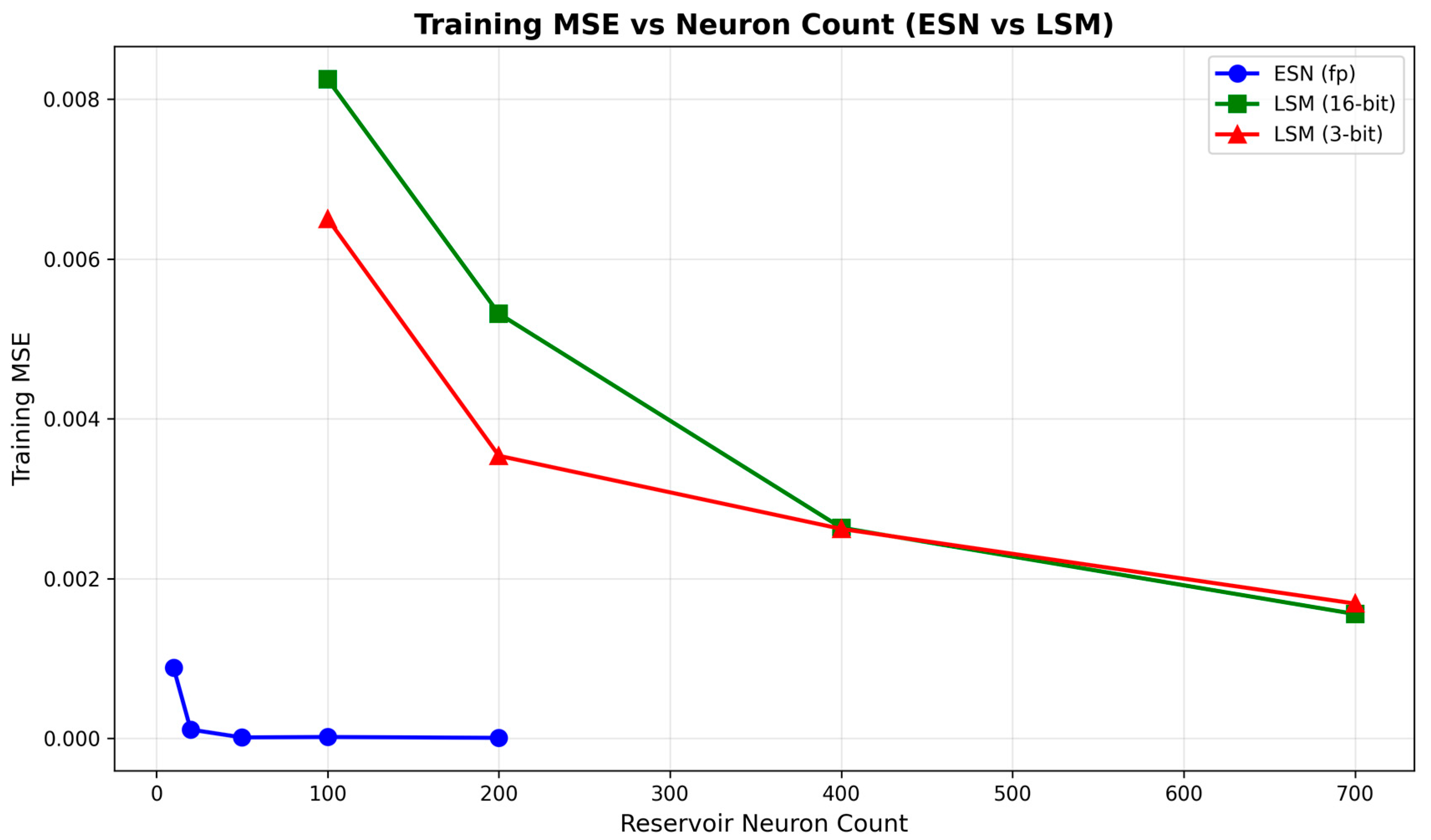
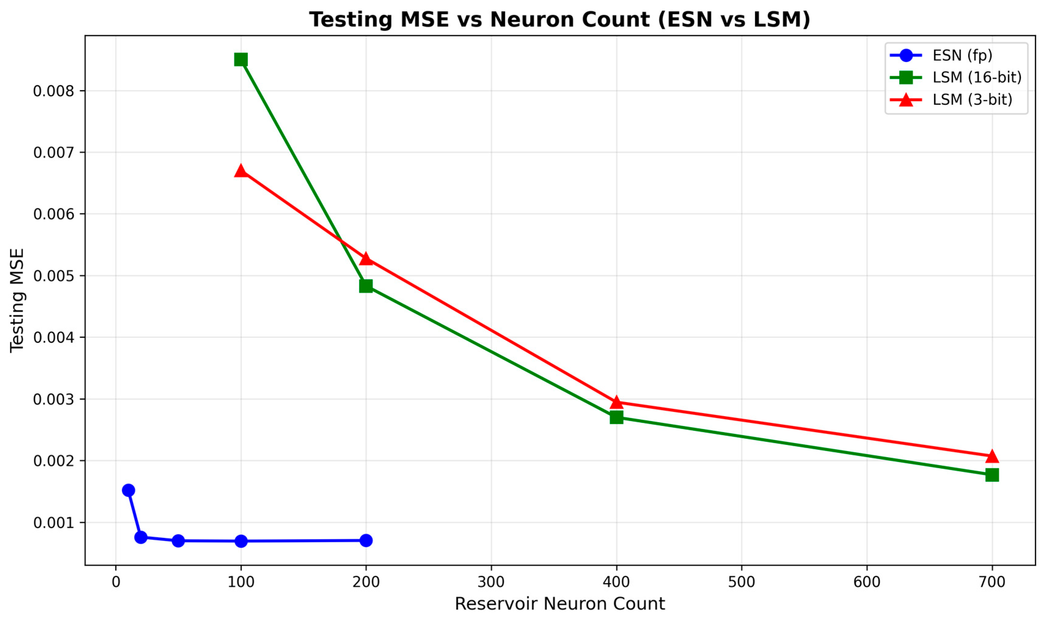
A direct comparison between ESN and LSM performance highlights differences in scaling behavior and robustness, as shown in
Figure 7 and
Figure 8. While the ESN achieves lower absolute MSE with relatively small reservoirs, its testing performance saturates early and shows limited improvement with increasing reservoir size. In contrast, the LSM exhibits a more gradual reduction in both training and testing MSE as the liquid size increases, indicating that larger spiking reservoirs continue to improve temporal representation. Consistent trends are also observed under MAE in the per-model results (
Figure 3,
Figure 4,
Figure 5 and
Figure 6), supporting the same conclusions regarding scalability and robustness.
Although the ESN achieves lower testing MSE in these experiments, the LSM exhibits more consistent performance trends across increasing reservoir size and reduced precision.
4.6. Hardware Implications of Reservoir Quantization
Beyond predictive accuracy, the observed robustness of RC models to reduced error precision has important implications for hardware-efficient implementation. Quantization directly impacts memory footprint, arithmetic complexity, and power consumption in digital and mixed-signal systems, making bit-width sensitivity a critical metric for hardware–software co-design.
For the ESN,
Figure 3 and
Figure 4 show that reducing reservoir weight precision from full precision to as low as 2-bit introduces only minor variation in training MSE and MAE. However, for testing MSE, lower-precision reservoirs exhibit a clearer degradation in generalization performance, with the 2-bit ESN showing an earlier increase in error as the reservoir size grows, indicating a stronger tendency toward overfitting compared to higher-precision implementations. This behavior suggests that ESN reservoirs tolerate moderate quantization without catastrophic degradation, particularly at small to medium reservoir sizes. However, ESNs rely on continuous-valued state updates and dense matrix–vector multiplications, which remain computationally expensive even under reduced precision. As a result, while quantization reduces memory usage, ESN inference still incurs significant arithmetic overhead in hardware implementations.
In contrast, the LSM demonstrates strong robustness to aggressive reservoir quantization across all evaluated liquid sizes, as shown in
Figure 5 and
Figure 6. Notably, the 3-bit LSM closely tracks the performance of the 16-bit configuration in both training and testing MSE and MAE, with performance gaps diminishing as liquid size increases. This behavior indicates that LSM dynamics are inherently resilient to low-precision representations, owing to their event-driven spiking activity, threshold-based computation, and sparse synaptic interactions.
From a hardware perspective, these results suggest that LSM reservoirs can be implemented using low-bit-width memory for synaptic weights, membrane potentials, and thresholds without significant loss in predictive performance. Such reductions translate directly into lower memory bandwidth requirements, reduced switching activity, and simplified arithmetic units. When combined with event-driven computation, low-precision LSMs offer a compelling pathway toward energy-efficient neuromorphic and edge computing systems. In contrast, while ESNs remain attractive for compact, high-accuracy deployments, their continuous-valued computation limits the achievable hardware efficiency gains from quantization alone.
4.7. Additional Benchmark (NARMA-10)
To further evaluate the performance and generalization capability of the ESN and the LSM under different dynamical conditions, we additionally benchmark both models using the NARMA-10 task.
4.7.1. Dataset
The NARMA-10 dataset is generated using the following nonlinear recurrence equation:
where u(n) denotes the input sequence drawn from an independent and identically distributed uniform distribution and y(n) represents the target output. The output at step n + 1 depends on the previous ten output values as well as delayed input terms, which imposes a strict requirement on the short-term memory and nonlinear processing capability of the reservoir.
For the segment used in our experiments (6000 samples), the NARMA-10 values have a minimum of 0.1711, maximum of 0.8110, mean of 0.3609, and variance of 0.0098. We applied normalization prior to training using parameters computed on the training split and applied consistently to the test split.
4.7.2. Evaluation for NARMA10 for ESN vs. LSM
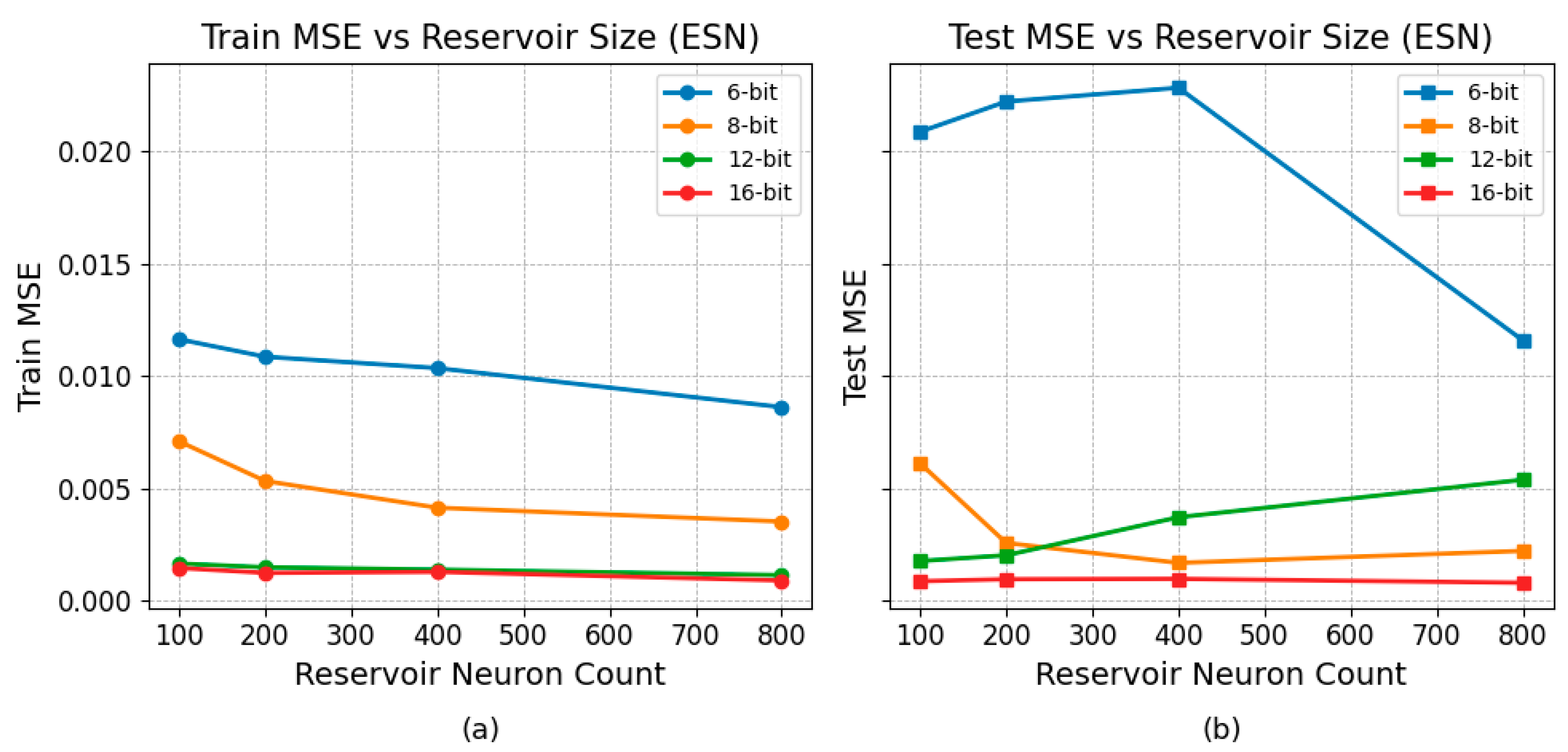
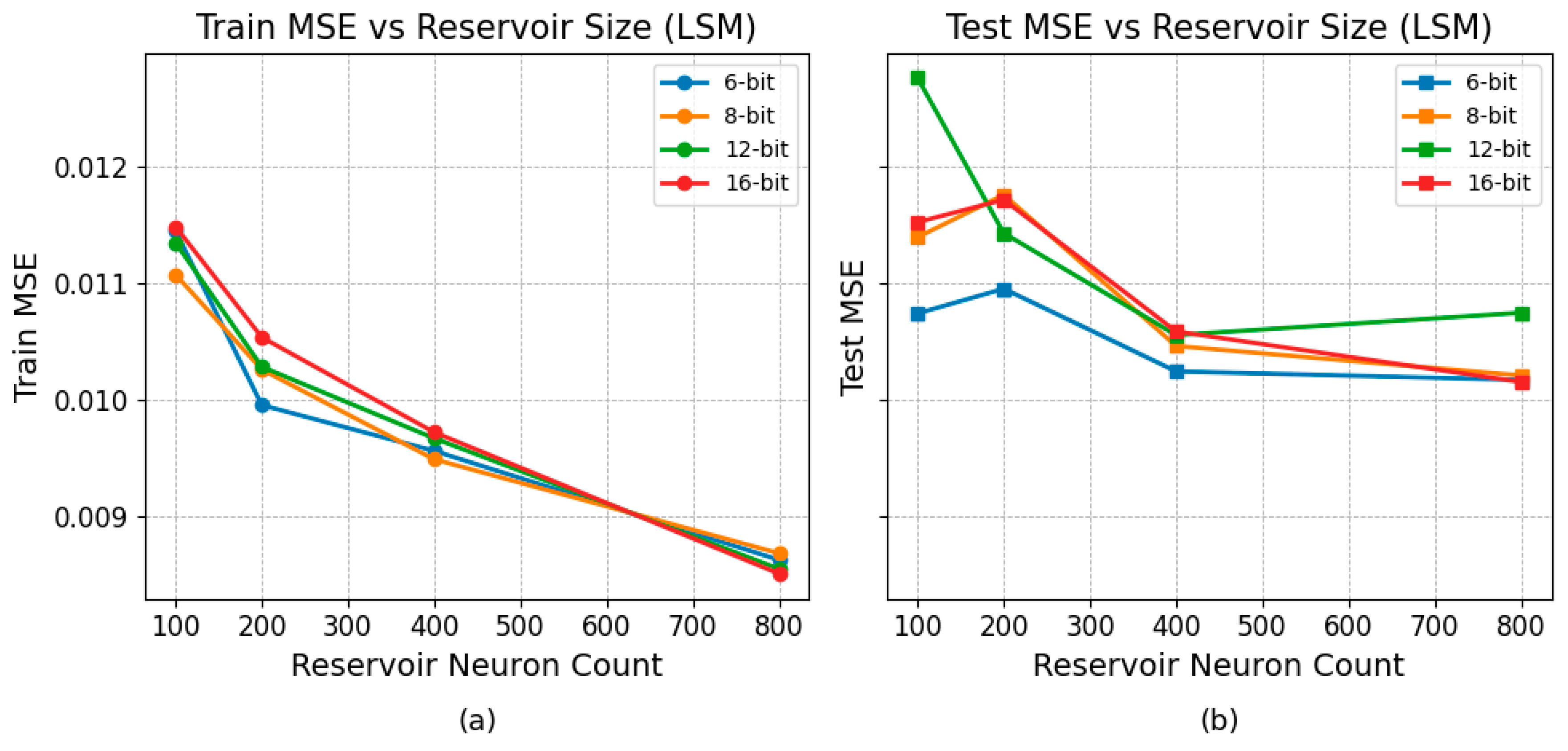
Figure 9 and
Figure 10 illustrate the training and testing MSE of the ESN and LSM on the NARMA-10 benchmark under varying reservoir sizes (100, 200, 400, 800) and weight quantization levels (6-bit, 8-bit, 12-bit, and 16-bit). Overall, the trends observed on the NARMA-10 dataset are highly consistent with those reported for the Mackey–Glass benchmark, indicating that the comparative behaviors of ESN and LSM generalize across different nonlinear temporal tasks.
For the ESN,
Figure 9a shows that increasing the reservoir size can reduce training MSE at the beginning, and it becomes stable when the size is large. Also, the corresponding testing MSE in
Figure 9b shows limited improvement and, in some cases, a mild increase as the reservoir grows, due to overfitting.
In contrast, the LSM exhibits a more balanced scaling behavior. As illustrated in
Figure 10, both training and testing MSE decrease steadily with increasing liquid reservoir size, and no significant separation between the two curves is observed.
Regarding the impact of weight quantization, its effect remains limited across the evaluated precision levels for the LSM, whereas a more noticeable influence is observed for the ESN.
Overall, the NARMA-10 results reinforce the key distinction between the two RC paradigms. These observations, consistent across both Mackey–Glass and NARMA-10 benchmarks, highlight fundamental differences in how continuous-valued and spiking reservoirs exploit increased model capacity for temporal modeling.
5. Discussion
The experimental results demonstrate distinct trade-offs between ESNs and LSMs when applied to chaotic time-series prediction.
An important observation is the tendency of ESNs to overfit under certain configurations, particularly when operating with reduced precision of reservoir weights. Although this behavior is often regarded as an inherent limitation of ESNs, it may be mitigated through stronger regularization techniques or sparsity-aware optimization methods.
Because the ESN readout is trained by ridge regression, we also swept the ridge regularization coefficient (
) during manual hyperparameter tuning through exhaustive experiments (see
Table 2 in
Section 4.3). Notably,
Table 2 confirms an appropriate β choice at a representative large reservoir size (
N = 200), but it does not change the broader trend that increasing ESN size yields limited additional test set gains beyond moderate reservoir sizes. Increasing
reduced variance in some settings, but it did not remove the early saturation/mild increase in test MSE observed at larger reservoir sizes, especially under low-bit quantization. This suggests that despite optimization of regularization parameters, the performance still depends upon quantization of reservoir as well as reservoir dynamics/sizes.
In contrast, the spiking nature of LSMs provides an implicit form of regularization, as information is encoded temporally through discrete events rather than continuous-valued activations. This characteristic has been shown to enhance robustness to noise and quantization in spiking neural networks and spiking reservoirs, making LSMs particularly suitable for deployment in low-power and resource-constrained environments [
7,
11,
17].
To examine whether these observations are task-dependent, we evaluated both models on the NARMA-10 benchmark and the Mackey–Glass chaotic time series, which are two widely adopted benchmarks for evaluating temporal prediction, nonlinear dynamics, and memory capacity in recurrent models [
5,
8,
18].
From a hardware perspective, the quantization resilience demonstrated by LSMs suggests potential advantages for neuromorphic and edge AI systems, where reduced memory precision and event-driven computation are critical for energy efficiency [
3,
11,
15]. Nevertheless, the present analysis focuses on algorithmic-level performance and does not explicitly account for full hardware-level costs. A comprehensive evaluation of these factors on pure hardware-based designs such as ASIC or FPGA prototype accelerators is necessary to fully characterize the end-to-end efficiency of spiking RC systems.
6. Conclusions, Limitations and Future Work
This study presents a systematic comparison between quantized Echo State Networks and Liquid State Machines for chaotic time-series prediction, with a particular focus on robustness to reduced numerical error precision and implications for neuromorphic and edge AI systems. By evaluating both models under identical experimental conditions, the study highlights fundamental trade-offs between predictive accuracy and hardware-oriented efficiency that are often overlooked in conventional full-precision evaluations.
The results indicate that while ESNs can achieve strong predictive performance under favorable conditions, their sensitivity to quantization and potential for overfitting may limit their suitability for low-power or resource-constrained deployments. In contrast, LSMs demonstrate greater robustness to reduced precision, benefiting from event-driven computation and spiking dynamics that naturally align with neuromorphic hardware architectures [
3,
7,
11]. These findings suggest that spiking RC models offer a promising pathway toward efficient temporal processing in edge and neuromorphic computing scenarios.
The novelty of this study lies in its unified benchmarking framework for comparing quantized ESN and LSM models, providing insights into how architectural and numerical limitation of reservoir weights manifest under realistic time-series applications. Rather than optimizing for absolute accuracy alone, this work emphasizes the importance of evaluating RC models through the lens of hardware efficiency, robustness, and deployability for practical time-series problems.
Future work will focus on validating these findings on real hardware. Although our analysis models hardware constraints by quantizing reservoir states/weights at different bit precisions, all experiments were conducted at an algorithmic level and therefore do not capture full-system effects such as communication overhead, memory access, timing, and on-chip learning feasibility. The next step is to implement ESN and LSM designs using RTL/HDL-based development flows and deploy FPGA prototypes to evaluate real-time hardware behavior.
This work contributes to the growing body of research on RC by clarifying the strengths and limitations of artificial and spiking reservoir models under quantization, and by providing guidance for selecting appropriate architectures as well as hyperparameter configurations in energy-constrained and hardware-oriented applications.
Author Contributions
Conceptualization, Y.Y.; methodology, A.L., M.F.A. and C.L.; software, A.L., M.F.A. and C.L.; validation, A.L., M.F.A. and C.L.; formal analysis, A.L., M.F.A. and C.L.; investigation, A.L., M.F.A. and C.L.; writing—original draft preparation, A.L., M.F.A. and C.L.; writing—review and editing, A.L., M.F.A., C.L. and Y.Y.; supervision, Y.Y.; project administration, Y.Y. All authors have read and agreed to the published version of the manuscript.
Funding
This research received no external funding.
Institutional Review Board Statement
Not applicable.
Informed Consent Statement
Not applicable.
Data Availability Statement
Conflicts of Interest
The authors declare no conflict of interest.
References
- Yan, M.; Huang, C.; Bienstman, P.; Tino, P.; Lin, W.; Sun, J. Emerging opportunities and challenges for the future of RC. Nat. Commun. 2024, 15, 2056. [Google Scholar] [CrossRef] [PubMed]
- Wahid, S.A.A.; Asad, A.; Mohammadi, F. A Survey on Neuromorphic Architectures for Running Artificial Intelligence Algorithms. Electronics 2024, 13, 2963. [Google Scholar] [CrossRef]
- Davies, M.; Srinivasa, N.; Lin, T.-H.; Chinya, G.; Cao, Y.; Choday, S.H.; Dimou, G.; Joshi, P.; Imam, N.; Jain, S.; et al. Loihi: A Neuromorphic Manycore Processor with On-Chip Learning. IEEE Micro 2018, 38, 82–99. [Google Scholar] [CrossRef]
- Akopyan, F.; Sawada, J.; Cassidy, A.; Alvarez-Icaza, R.; Arthur, J.; Merolla, P.; Imam, N.; Nakamura, Y.; Datta, P.; Nam, G.-J.; et al. TrueNorth: Design and Tool Flow of a 65 mW 1 Million Neuron Programmable Neurosynaptic Chip. IEEE Trans. Comput. Des. Integr. Circuits Syst. 2015, 34, 1537–1557. [Google Scholar] [CrossRef]
- Benjamin, B.V.; Gao, P.; McQuinn, E.; Choudhary, S.; Chandrasekaran, A.R.; Bussat, J.-M.; Alvarez-Icaza, R.; Arthur, J.V.; Merolla, P.A.; Boahen, K. Neurogrid: A Mixed-Analog-Digital Multichip System for Large-Scale Neural Simulations. Proc. IEEE 2014, 102, 699–716. [Google Scholar] [CrossRef]
- Qiao, N.; Mostafa, H.; Corradi, F.; Osswald, M.; Stefanini, F.; Sumislawska, D.; Indiveri, G. A reconfigurable on-line learning spiking neuromorphic processor comprising 256 neurons and 128K synapses. Front. Neurosci. 2015, 9, 141. [Google Scholar] [CrossRef]
- EChicca, E.; Stefanini, F.; Bartolozzi, C.; Indiveri, G. Neuromorphic Electronic Circuits for Building Autonomous Cognitive Systems. Proc. IEEE 2014, 102, 1367–1388. [Google Scholar] [CrossRef] [PubMed]
- Antonelo, E.A.; Schrauwen, B.; Stroobandt, D. Event detection and localization for small mobile robots using RC. Neural Netw. 2008, 21, 862–871. [Google Scholar] [CrossRef] [PubMed]
- Jaeger, H. The ‘Echo State’ Approach to Analysing and Training Recurrent Neural Networks; GMD Report 148; German National Research Center for Information Technology (GMD): Sankt Augustin, Germany, 2001. [Google Scholar]
- Goodfellow, I.; Bengio, Y.; Courville, A. Deep Learning; MIT Press: Cambridge, MA, USA, 2016; Available online: https://www.deeplearningbook.org (accessed on 9 February 2026).
- Bohte, S.M.; Kok, J.N.; La Poutre, H. Error-backpropagation in temporally encoded networks of spiking neurons. Neurocomputing 2002, 48, 17–37. [Google Scholar] [CrossRef]
- Jaeger, H.; Haas, H. Harnessing nonlinearity: Predicting chaotic systems and saving energy in wireless communication. Science 2004, 304, 78–80. [Google Scholar] [CrossRef] [PubMed]
- Indiveri, G.; Linares-Barranco, B.; Legenstein, R.; Deligeorgis, G.; Prodromakis, T. Integration of nanoscale memristor synapses in neuromorphic computing architectures. Front. Neurosci. 2013, 24, 384010. [Google Scholar] [CrossRef] [PubMed]
- Maass, W.; Natschläger, T.; Markram, H. Real-time computing without stable states: A new framework for neural computation based on perturbations. Neural Comput. 2002, 14, 2531–2560. [Google Scholar] [CrossRef] [PubMed]
- Deckers, L.; Tsang, I.J.; Van Leekwijck, W.; Latré, S. Extended Liquid State Machines for Speech Recognition. Front. Neurosci. 2022, 16, 1023470. [Google Scholar] [CrossRef] [PubMed]
- Gan, V.M.; Liang, Y.; Li, L.; Liu, L.; Yi, Y. A Cost-Efficient Digital Echo State Network Architecture on FPGA for OFDM Symbol Detection. ACM J. Emerg. Technol. Comput. Syst. 2021, 17, 34. [Google Scholar] [CrossRef]
- Voshol, J.M. Quantized Liquid State Machines. GitHub Repository, 2025. Available online: https://github.com/m4urin/quantized-liquid-state-machines (accessed on 9 February 2026).
- Thill, M.; Konen, W.; Bäck, T. MarkusThill/MGAB: The Mackey-Glass Anomaly Benchmark. Zenodo, version v1.0.1. 2020. Available online: https://zenodo.org/records/3762385 (accessed on 9 February 2026).
- Mackey, M.; Glass, L. Oscillation and chaos in physiological control systems. Science 1977, 197, 287–289. [Google Scholar] [CrossRef] [PubMed]
Figure 1.
Echo State Network (ESN) architecture illustrating the transformation from the input signal , through the recurrent reservoir state , to the output . The diagram highlights the fixed input weights , recurrent reservoir weights , and trained readout weights , which together enable nonlinear temporal processing through high-dimensional reservoir dynamics.
Figure 1.
Echo State Network (ESN) architecture illustrating the transformation from the input signal , through the recurrent reservoir state , to the output . The diagram highlights the fixed input weights , recurrent reservoir weights , and trained readout weights , which together enable nonlinear temporal processing through high-dimensional reservoir dynamics.
Figure 2.
LSM processing pipeline for temporal signal prediction. A continuous-valued input signal is first converted into spike trains through an encoding stage. The resulting input spikes drive a recurrent spiking reservoir (the liquid), where leaky integrate-and-fire neurons generate rich spatio-temporal dynamics. Reservoir spike activity is subsequently decoded into continuous-valued state representations, which are mapped to the final output through a linear readout layer to produce the predicted signal.
Figure 2.
LSM processing pipeline for temporal signal prediction. A continuous-valued input signal is first converted into spike trains through an encoding stage. The resulting input spikes drive a recurrent spiking reservoir (the liquid), where leaky integrate-and-fire neurons generate rich spatio-temporal dynamics. Reservoir spike activity is subsequently decoded into continuous-valued state representations, which are mapped to the final output through a linear readout layer to produce the predicted signal.
Figure 3.
Training MSE and MAE versus reservoir neuron count for the ESN on the Mackey–Glass task. Results are shown for full-precision and quantized reservoir weights.
Figure 3.
Training MSE and MAE versus reservoir neuron count for the ESN on the Mackey–Glass task. Results are shown for full-precision and quantized reservoir weights.
Figure 4.
Testing MSE and MAE versus reservoir neuron count for the ESN on the Mackey–Glass task. Quantized reservoir weights maintain comparable generalization performance to full precision.
Figure 4.
Testing MSE and MAE versus reservoir neuron count for the ESN on the Mackey–Glass task. Quantized reservoir weights maintain comparable generalization performance to full precision.
Figure 5.
Training MSE and MAE versus liquid neuron count for the LSM under different quantization levels. Larger liquid sizes consistently reduce training error.
Figure 5.
Training MSE and MAE versus liquid neuron count for the LSM under different quantization levels. Larger liquid sizes consistently reduce training error.
Figure 6.
Testing MSE and MAE versus liquid neuron count for the LSM under different quantization levels. Low-precision LSMs closely track full-precision performance as liquid size increases.
Figure 6.
Testing MSE and MAE versus liquid neuron count for the LSM under different quantization levels. Low-precision LSMs closely track full-precision performance as liquid size increases.
Figure 7.
Training MSE versus reservoir neuron count comparing ESN (full precision) and LSM (16-bit and 3-bit). The ESN converges rapidly, while the LSM improves gradually with size.
Figure 7.
Training MSE versus reservoir neuron count comparing ESN (full precision) and LSM (16-bit and 3-bit). The ESN converges rapidly, while the LSM improves gradually with size.
Figure 8.
Testing MSE versus reservoir neuron count comparing ESN and LSM. The LSM demonstrates scalable generalization and robustness to low-precision reservoir representations.
Figure 8.
Testing MSE versus reservoir neuron count comparing ESN and LSM. The LSM demonstrates scalable generalization and robustness to low-precision reservoir representations.
Figure 9.
The (a) training performance and (b) testing performance of ESN at different reservoir sizes and different quantization bits.
Figure 9.
The (a) training performance and (b) testing performance of ESN at different reservoir sizes and different quantization bits.
Figure 10.
The (a) training performance and (b) testing performance of LSM at different reservoir sizes and different quantization bits.
Figure 10.
The (a) training performance and (b) testing performance of LSM at different reservoir sizes and different quantization bits.
Table 1.
Hyperparameters and experimental settings used in ESN and LSM experiments.
Table 1.
Hyperparameters and experimental settings used in ESN and LSM experiments.
| Category | ESN | LSM |
|---|
| Train/test split | 5000/1000 (contiguous) | 5000/1000 (contiguous) |
| Reservoir sizes swept | | |
| Quantization levels swept | -bit | -bit |
| Random seeds | Fixed seed (SEED = 42) | Fixed seed (SEED = 42) |
| State update/leak parameter | | |
| Reservoir weights | , signed by neuron type | , signed by neuron type |
| Regularization/optimizer | | Adam optimizer |
| Training epochs | 1 epoch (closed-form ridge solve) | 500 epochs |
Table 2.
ESN ridge regularization sweep () at N = 200 under full precision and 2-bit quantization (test MSE).
Table 2.
ESN ridge regularization sweep () at N = 200 under full precision and 2-bit quantization (test MSE).
| (Ridge) | Test MSE (Full Precision) | Test MSE (2-bit) |
|---|
| | |
| | |
| | |
| | |
| | |
| | |
| | |
| | |
| Disclaimer/Publisher’s Note: The statements, opinions and data contained in all publications are solely those of the individual author(s) and contributor(s) and not of MDPI and/or the editor(s). MDPI and/or the editor(s) disclaim responsibility for any injury to people or property resulting from any ideas, methods, instructions or products referred to in the content. |