Detection of Cracks in Low-Power Wind Turbines Using Vibration Signal Analysis with Empirical Mode Decomposition and Convolutional Neural Networks

Abstract

Condition monitoring and fault detection in wind turbines are essential for reducing repair and maintenance costs. Early detection of faults enables timely interventions before the damage worsens. However, existing methods often rely on costly scheduled inspections or lack the ability to effectively detect early stage damage, particularly under different operational speeds. This article presents a methodology based on convolutional neural networks (CNNs) and empirical mode decomposition (EMD) of vibration signals for the detection of blade crack damage. The proposed approach involves acquiring vibration signals under four conditions: healthy, light, intermediate, and severe damage. EMD is then applied to extract time–frequency representations of the signals, which are subsequently converted into images. These images are analyzed by a CNN to classify the condition of the wind turbine blades. To enhance the final CNN architecture, various image sizes and configuration parameters are evaluated to balance computational load and classification accuracy. The results demonstrate that combining vibration signal images, generated using the EMD method, with CNN models enables accurate classification of blade conditions, achieving 99.5% accuracy while maintaining a favorable trade-off between performance and complexity.

1. Introduction

In recent decades, the use of renewable energy has steadily increased as a strategy to reduce dependence on fossil fuels and mitigate the rise in carbon dioxide emissions [1]. Currently, renewables account for approximately 30% of global electricity generation, with wind energy representing one of the most significant contributors, supplying around 7.8% [2,3]. However, the operational challenges and maintenance costs associated with wind turbines, particularly concerning blade integrity, remain significant obstacles to wider adoption [4,5]. Existing methods for blade damage detection often rely on costly scheduled inspections or lack the sensitivity to identify early stage damage effectively [6,7]. This highlights a critical research gap: the need for automated, cost-effective, and sensitive methods for detecting blade cracks in wind turbines, enabling proactive maintenance and minimizing downtime [8,9,10].

Several factors can compromise the structural integrity of wind turbine blades, including temperature fluctuations, mechanical loads, harsh environmental conditions such as humidity, dust, and icing, as well as interactions with birds or other wildlife. These factors may lead to crack formation, which, if not detected early, can propagate and result in catastrophic failure [11,12,13]. Traditionally, basic damage inspection has been performed through periodic visual analysis. However, some faults, especially in their early stages, are not visible to the naked eye [14,15]. As a result, the analysis and detection of incipient damage in wind turbines have become increasingly relevant for implementing effective preventive maintenance strategies.

Vibration signal analysis provides valuable insights into the structural condition of turbine blades by capturing their dynamic response to wind profiles. Given the high information content in these signals, they are widely used for structural health monitoring and fault diagnosis in wind turbines [16,17]. Among the different types of faults, this work specifically focuses on blade damage, which accounts for 19.4% of all reported faults in wind turbines [9,18]. Considering that vibration signals contain dynamic characteristics of the system, they are particularly suitable for analyzing rotating components such as turbine blades [19].

In general, two main approaches are commonly used in wind turbine fault analysis: machine learning (ML) and deep learning. In the context of ML, Xu et al. [20] conducted structural health monitoring using acoustic signals, applying algorithms such as support vector machines (SVM) and distributed acoustic sensing (DAS). Similarly, Tang et al. [21] used the k-nearest neighbors (KNN) algorithm combined with generalized fractal dimensions (GFD) to detect blade damage. Despite obtaining promising results, the effectiveness of ML models depends heavily on the selection of input features, which poses a significant challenge due to the vast number of possible descriptors that can be extracted, including statistical indices, fractal-based measures, entropy metrics, and more [6]. To overcome these limitations, deep learning techniques have gained prominence. Unlike traditional ML methods, deep learning models can automatically extract relevant features during training. In this regard, deep learning has been extensively applied in image recognition tasks, particularly using photographs captured by UAV for structural damage assessment. For instance, Xiang et al. [22] proposed a crack detection framework using UAV images, applying LogitBoost and SVM classifiers. Similarly, Reddy et al. [23] used convolutional neural networks (CNNs) to detect blade cracks in UAV images, while Tung-Chen et al. [24] developed a CNN-based system to detect damage in commercial wind turbines using acoustic signals and spectrograms. Finally, Shihavuddin et al. [25] also employed CNNs for comprehensive image-based damage detection in turbine structures.

Although these approaches have shown excellent results, continuous condition monitoring based on UAV is not always feasible due to operational constraints and high costs. As a result, research has increasingly focused on vibration-based monitoring, which allows for continuous data acquisition through fixed sensors and is more suitable for real-time applications. To leverage the advantages of deep learning in this context, a common strategy involves transforming vibration signals into time–frequency images, thereby enabling the use of image-based CNN architectures for effective fault classification. One widely used technique for this purpose is the short-time Fourier transform (STFT), which enables the generation of spectrograms that capture the time–frequency characteristics of non-stationary signals [26]. Among the advantages of STFT are its relatively simple implementation and its capacity to represent signal evolution over time. However, STFT also presents notable limitations, such as the fixed resolution trade-off between time and frequency, and potential loss of detail for rapidly changing signal components. To overcome these drawbacks, other signal processing techniques have been explored. One method that has shown promising results in a variety of domains is the empirical mode decomposition (EMD) and its extensions. EMD is a fully data-driven and adaptive approach capable of decomposing complex signals into intrinsic mode functions (IMFs) without requiring a predefined basis. These IMFs preserve local oscillatory modes without prior assumptions, which is particularly useful for detecting early stage damage. In particular, Dao et al. [27] proposed a method combining wavelet thresholding with ensemble EMD to characterize error signals, while Wang et al. [28] also used ensemble EMD in conjunction with blade natural frequencies to assess dynamic behavior. Given the effectiveness demonstrated by EMD-based approaches, it is scientifically relevant to explore EMD as a signal-to-image transformation method to feed CNN architectures for fault classification, particularly for detecting cracks in wind turbine blades at different severity levels, with emphasis on incipient damage. Moreover, considering that most existing studies are limited to fixed wind turbine speed conditions, evaluating the performance of such approaches under multiple wind turbine speed levels offers a valuable and relatively unexplored research direction.

Building upon the discussion above, this work proposes a methodology based on vibration signal analysis using EMD to generate images as input for a CNN aimed at detecting blade cracks at different severity levels. EMD decomposes the vibration signals into a set of IMFs, enabling an adaptive time–frequency representation of the signal. These IMFs are then used to construct images, which are processed by a CNN to classify the condition of the wind turbine blades under three different wind turbine angular speed levels (3, 7, and 12 revolutions per second, rps). The damage conditions considered correspond to the progression of a crack through four stages: healthy and light, intermediate, and severe damage. In addition, different CNN architectures and input image sizes were evaluated in order to reduce model complexity without compromising classification accuracy. The results demonstrate an average classification accuracy of 99.5% across all wind turbine angular speed levels, while maintaining a favorable trade-off between accuracy and complexity.

2. Theoretical Background

This section presents the key concepts underlying the present work, including a brief overview of wind turbines and the signal processing and classification techniques used for crack detection.

2.1. Wind Turbine

A wind turbine is a rotating machine that converts the kinetic energy of wind into electrical energy. The most common and efficient configuration is the horizontal axis wind turbine (HAWT), which is favored for its high energy conversion efficiency and substantial power generation capacity. In this design, the rotor’s axis of rotation is parallel to the ground [29]. Typically, the turbine includes a rotating shaft mounted at the top of a tower, which requires a yaw mechanism to align the rotor with varying wind directions.

The main components of a HAWT include the rotor blades and the rotor hub, which together form the primary power generating unit. The blades are susceptible to imbalance caused by various factors, such as manufacturing or installation defects, environmental interactions (e.g., bird strikes), and operational wear [30].

Vibration signals are widely used for monitoring the structural health of wind turbines. By analyzing these signals, faults such as imbalance, misalignment, and structural damage can be identified. It is therefore crucial to understand the characteristic patterns embedded in these vibratory responses.

One common source of vibration is the tower shadow effect, which occurs when the blades pass in front of the tower, causing periodic disturbances in the vibration signal. This phenomenon is commonly modeled as follows [31]:

$$v\left(t\right)=\sum _{m=1}^M{A}_m\mathrm{s}\mathrm{i}\mathrm{n}\left(m\omega t+{\phi }_m\right)+\sum _{n=1}^N{A}_n\sin \left(3n\omega t+{\phi }_n\right)$$

(1)

This equation is defined as follows:

• The first summation represents the imbalance of the rotating parts.
• The second summation represents the impact of the tower.
• $\omega$ and $t$ are the angular frequency and the time, respectively.
• $M$ and $N$ are the total number of components considered in each sum (rotor and tower, respectively).
• $m$ and $n$ are the indices of the sums for the rotor and the tower effect, respectively.
• $A_m$ and $A_n$ are the vibration amplitudes, while ${\phi }_m$ and ${\phi }_n$ represent the corresponding phase angles of the rotor and tower effects, respectively.

Once the vibration signals are captured, they are processed using the EMD technique to extract time–frequency features for fault detection and classification.

2.2. Empirical Mode Decomposition

The EMD method is a signal processing strategy suitable for the analysis of transient signals with nonlinear temporal and transient characteristics. EMD can decompose a time signal into a set of frequency bands called IMFs. Two conditions must be met for a set of frequency bands to be regarded as IMFs [32].

(a)

The number of zero crossings and extremes in the time signal should be at most equal to or different from 1.

(b)

The mean value of the upper and lower envelopes must be zero.

To extract each IMF, a procedure known as the sifting process is applied. This method is described below:

• Find the extremes (local high and low points) of the original signal $x\left(t\right)$.
• Connect the points shown in (i) with a cubic spline to find the upper and lower envelopes. The average of the two envelopes called $m_1$ is subtracted from the original time signal $x\left(t\right)$ to obtain a new time signal $h_1\left(t\right)$.

  $$h_1\left(t\right)=x\left(t\right)-m_1\left(t\right)$$

  (2)
• If $h_1 \left(t\right)$ does not satisfy conditions (a) and (b), steps (i) and (ii) are repeated until $h_k \left(t\right)$ satisfies both conditions. In this case, $h_k \left(t\right)$ is defined as the initial IMF:

  $$c_1\left(t\right)=h_k\left(t\right)={IMF}_1$$

  (3)
• After the first frequency band or ${IMF}_1$ is obtained, the signal $c_1\left(t\right)$ is subtracted from the original time signal $x\left(t\right)$ to calculate the remaining signal $r_1\left(t\right)$ as follows:

  $$r_1\left(t\right)=x\left(t\right)-c_1\left(t\right)$$

  (4)
• Prove that $r_1\left(t\right)$ is a monotonic function indicating that no more IMFs can be found. If $r_1\left(t\right)$ is not a unique function, treat it as a real-time signal and repeat steps (i) through (iii) to estimate other IMFs. The process terminates when $r_1\left(t\right)$ becomes a unitary function.
• Once the process is stopped, the original time signal $x\left(t\right)$ is decomposed into $N$ intrinsic modes, IMFs, and the last residue $r_N\left(t\right)$ as follows:

  $$x\left(t\right)=\sum _{n=1}^N{c}_n\left(t\right)+r_N\left(t\right)$$

  (5)

Thus, the EMD method is used to decompose the vibration signals into a set of IMFs, which are then used to construct time–frequency images that serve as input to a CNN for damage classification.

2.3. Convolutional Neural Networks

A CNN is a deep neural network architecture inspired by the human visual system. CNNs have been widely used since the early 2000s, achieving outstanding results in tasks such as segmentation, detection, and classification of objects and image regions [33]. This type of architecture is specifically designed to process structured data, particularly grid-like data such as images [33]. Compared to traditional ML algorithms, such as artificial neural networks, or recurrent neural networks (RNNs) and long short-term memory (LSTM) models, which are effective for sequential data, CNNs offer several advantages, including automatic feature extraction, strong representation capabilities, a deep hierarchical structure, nonlinear layers, pooling, and dropout mechanisms. Moreover, due to the local connectivity and weight sharing between neurons, a CNN requires fewer parameters, which reduces the complexity of optimization [34].

A typical CNN architecture consists of several stages. It begins with convolutional layers followed by pooling layers and ends with fully connected layers. A convolutional layer contains a set of filters (or kernels) $w$, which convolve over the input $x$ to generate a feature map through an activation function $f$. This operation can be mathematically described as follows:

$$y=f\left(\sum w\ast x+b\right)$$

(6)

where $b$ denotes the bias term.

After each convolutional operation, a pooling layer (typically max pooling) reduces the dimensionality of the feature map by retaining only the maximum value within each local region. This step reduces computational load and helps mitigate overfitting [26].

The output of the final pooling layer is flattened into a one-dimensional vector and passed to one or more fully connected layers, where each neuron is connected to every neuron in the previous layer. The final output layer computes class probabilities using an activation function such as ReLU or SoftMax. The SoftMax function normalizes the output into a probability distribution across $K$ classes, as expressed in the following equation [35]:

$$P\left(y=j|x;w_j,b_j\right)={\displaystyle \frac{e^{x\ast w_j+b_j}}{{\sum }_{k=1}^K{e}^{x\ast w_k+b_k}}}$$

(7)

Once the architecture and hyperparameters are defined, the network is trained using backpropagation, which computes gradients of the loss function to update weights across layers. CNN performance is typically evaluated using the root mean square (RMS) error and inter-class entropy. The training process aims to optimize learnable parameters such as the learning rate and the number of epochs. Figure 1 illustrates the architecture of the CNN used in this study.

3. Methodology

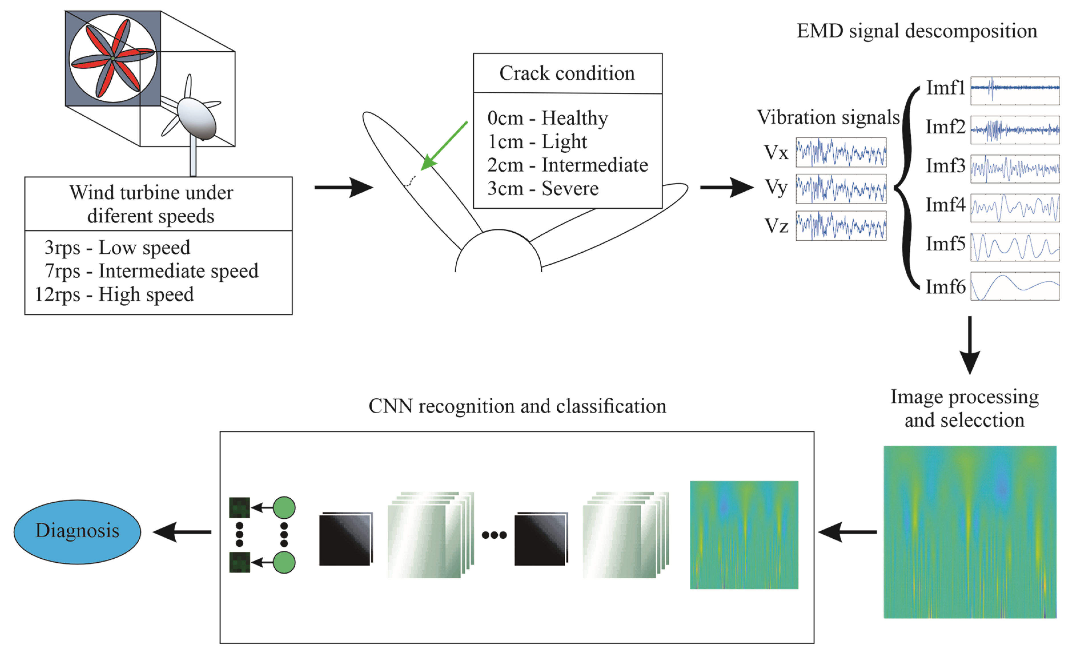
Figure 2 illustrates the proposed methodology, which is based on the analysis of vibration signals generated by crack damage in the blades of a low-power wind turbine. The study considers four blade conditions: healthy, light, intermediate, and severe damage which correspond to 0 cm, 1 cm, 2 cm, and 3 cm of crack longitude, respectively. Each condition is evaluated under three wind turbine angular speed levels, corresponding to the turbine’s start-up speed (3 rps), intermediate speed (7 rps), and maximum steady-state speed (12 rps). Vibration signals are captured using a tri-axial accelerometer mounted at the top of the wind turbine nacelle. These signals are then processed using EMD to extract IMFs, which are subsequently used to generate time–frequency images. Finally, the resulting images are analyzed by a CNN to identify the most suitable axis for fault classification.

To train the CNN, the largest image size (512 × 512 pixels) was used for each vibration signal axis, with the objective of identifying both the most informative axis and the optimal configuration for CNN training. During this process, the filter size and the number of filters were adjusted as tunable hyperparameters.

The experimental setup consists of a wind tunnel capable of generating three distinct wind speeds which produce three different angular speeds in the wind turbine: 3 rps, 7 rps, and 12 rps, corresponding to the turbine’s start-up, intermediate, and maximum steady-state speeds, respectively. The wind turbine used is a low-power air model rated at 12 V and 400 W. One of the blades was progressively damaged to simulate crack propagation. The entire turbine assembly was mounted on a rigid external base fixed to the ground to minimize turbulence generated during wind tunnel operation.

A Kistler 8395A10 accelerometer was installed over the turbine nacelle to capture vibration signals. Data acquisition was carried out using a National Instruments USB-6211 data acquisition (DAQ) board, with a sampling rate of 10,000 samples per second. All experiments were conducted on a computer equipped with a 2.30 GHz CPU, 16 GB of RAM, and a 64-bit operating system. Signal processing and CNN implementation were performed using MATLAB 2023a.

Figure 3 illustrates the experimental setup used in this study. The wind tunnel produces controlled airflow profiles, and the wind turbine is positioned at the outlet for testing. Two sets of blades were used: one in healthy condition and another exhibiting progressive levels of crack damage. To prevent external disturbances during testing, the turbine was securely mounted on a rigid base.

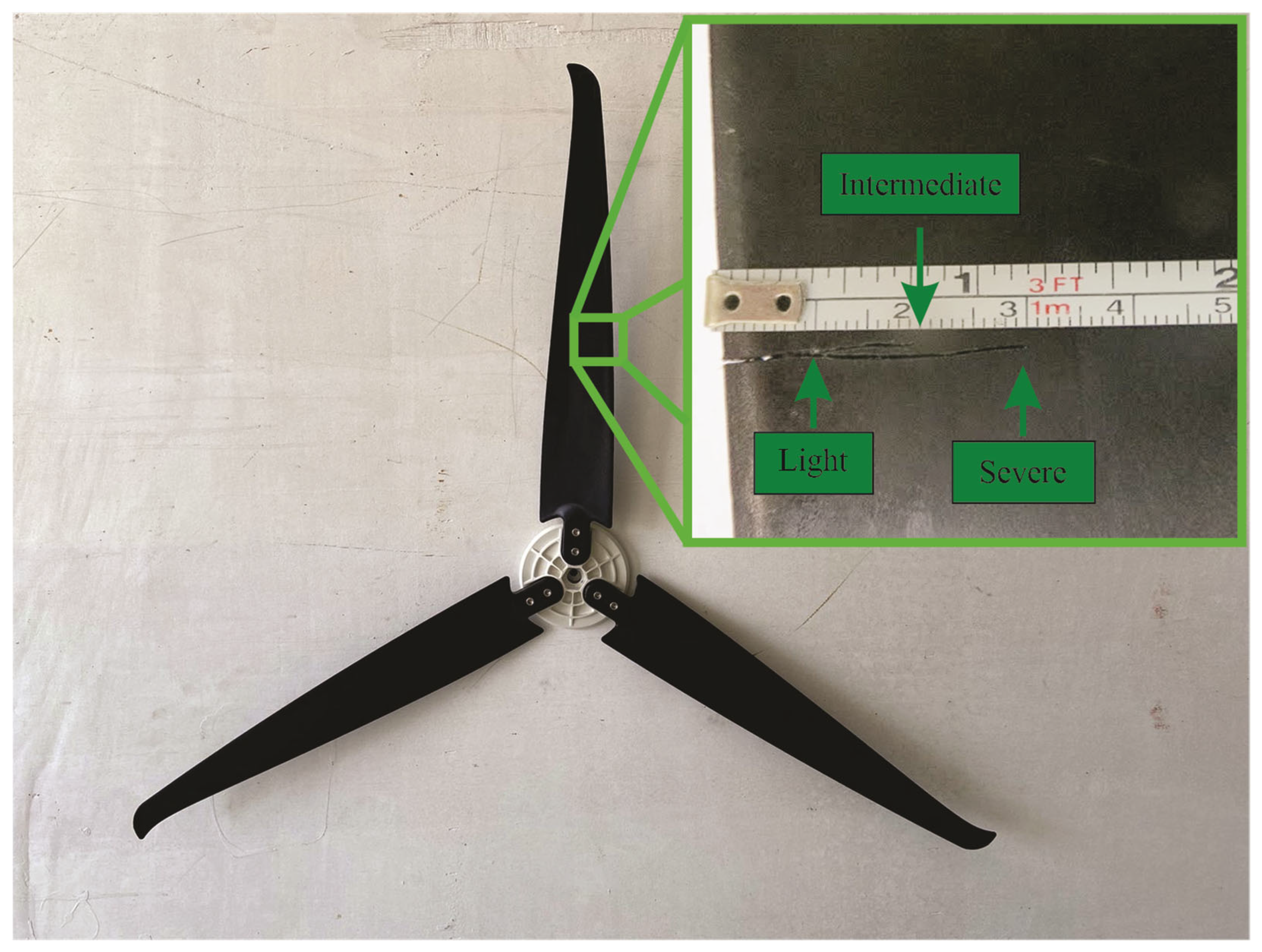
To simulate crack damage, one part of the wind turbine blade was progressively cut, as illustrated in Figure 4. Only one blade of the wind turbine was modified for this purpose. Tests were first conducted on the healthy blade (0 cm cut). Then, a 1 cm cut was introduced to simulate a light damage condition, and new tests were performed. Subsequently, the cut was deepened by an additional 1 cm to represent the next severity level, and the corresponding tests were carried out. This process was repeated until data were collected for all four damage classes. The procedure generated four distinct conditions representing increasing levels of damage:

• Healthy (0 cm);
• Light damage (1 cm);
• Intermediate damage (2 cm);
• Severe damage (3 cm).

These four cases, one non-damage (healthy) and three damage levels (light, intermediate and severe damage), were used for analysis. All cuts were made using a watchmaker’s wire saw. The length of each cut was gradually increased to emulate the progression of a crack, as stated above. The resulting fissures were subtle and, in some cases, nearly imperceptible to the naked eye, requiring close visual inspection to confirm their presence and extent. Figure 4 shows the visual appearance of the blade under each damage level.

4. Results

4.1. Vibration Signals

In this study, vibration signals were collected according to the test matrix presented in

Table 1. Test distribution.

Condition	Speed	X Axis	Y Axis	Z Axis
Healthy	3 rps	1000	1000	1000
	7 rps	1000	1000	1000
	12 rps	1000	1000	1000
Light damage	3 rps	1000	1000	1000
	7 rps	1000	1000	1000
	12 rps	1000	1000	1000
Intermediate damage	3 rps	1000	1000	1000
	7 rps	1000	1000	1000
	12 rps	1000	1000	1000
Severe damage	3 rps	1000	1000	1000
	7 rps	1000	1000	1000
	12 rps	1000	1000	1000
	Total	12,000	12,000	12,000

, which ensures a balanced dataset for each axis and damage level, enabling consistent evaluation of the classification model. Blade condition was divided into four levels: healthy and light, intermediate, and severe damage. Each condition was tested under three wind speed levels, i.e., low, intermediate, and high, with 1000 vibration signals acquired with 1200 samples per condition, resulting in a total of 12,000 signals. It is important to note, however, that while the tests were conducted under controlled conditions, each run inherently included acquisition and ambient noise, factors often overlooked in experimental setups. These sources of variation help simulate real-world system conditions, closely resembling the effects observed in data augmentation experiments, where the addition of Gaussian white noise produced results similar to those naturally present in the acquired data. The directions of the corresponding axes are shown in Figure 3.

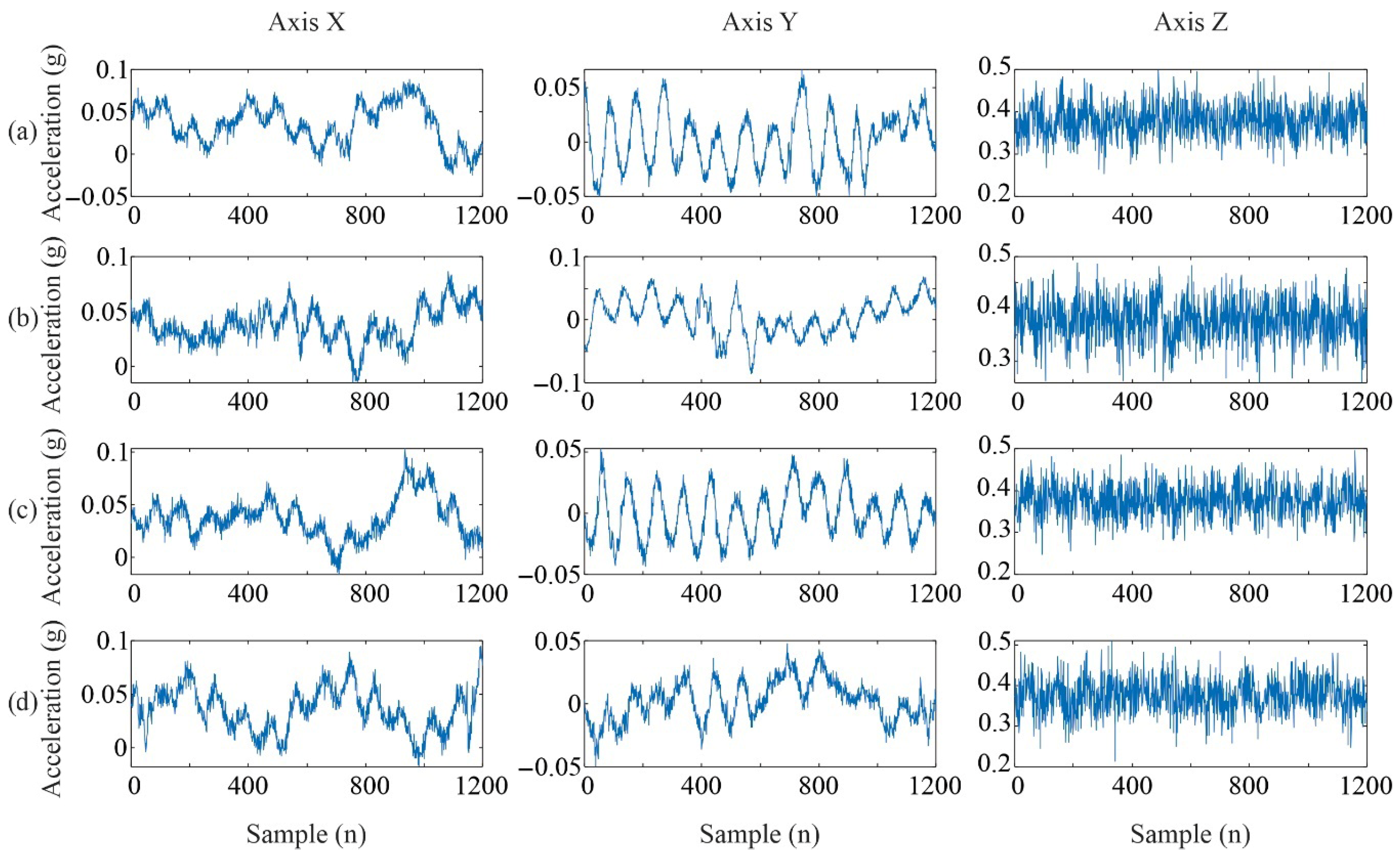
Figure 5 illustrates how the vibration signals vary depending on blade condition. As damage severity increases, differences in amplitude and signal shape become more noticeable. These patterns are later captured through EMD to generate the image representations used for classification.

The evaluated rotational speeds were 3 rps (180 rpm), 7 rps (420 rpm), and 12 rps (720 rpm), covering the full operational range of the wind turbine (~3 to 12 rps). In all tests, the turbine started from 0 rps, and data acquisition began once the system reached the target speed and a steady-state condition was achieved.

It is important to note that the crack simulation used in this study, introduced through precise cuts of 1 cm, 2 cm, and 3 cm at a fixed location, was designed to isolate the effect of damage severity on vibration signals. This simplified approach enabled the generation of controlled data to assess the feasibility of classification. Moreover, it provided a baseline understanding of the system’s vibrational response to varying degrees of crack severity, serving as a foundation for future, more complex analyses.

4.2. Pre-Processing of Vibration Signals and Image Generation

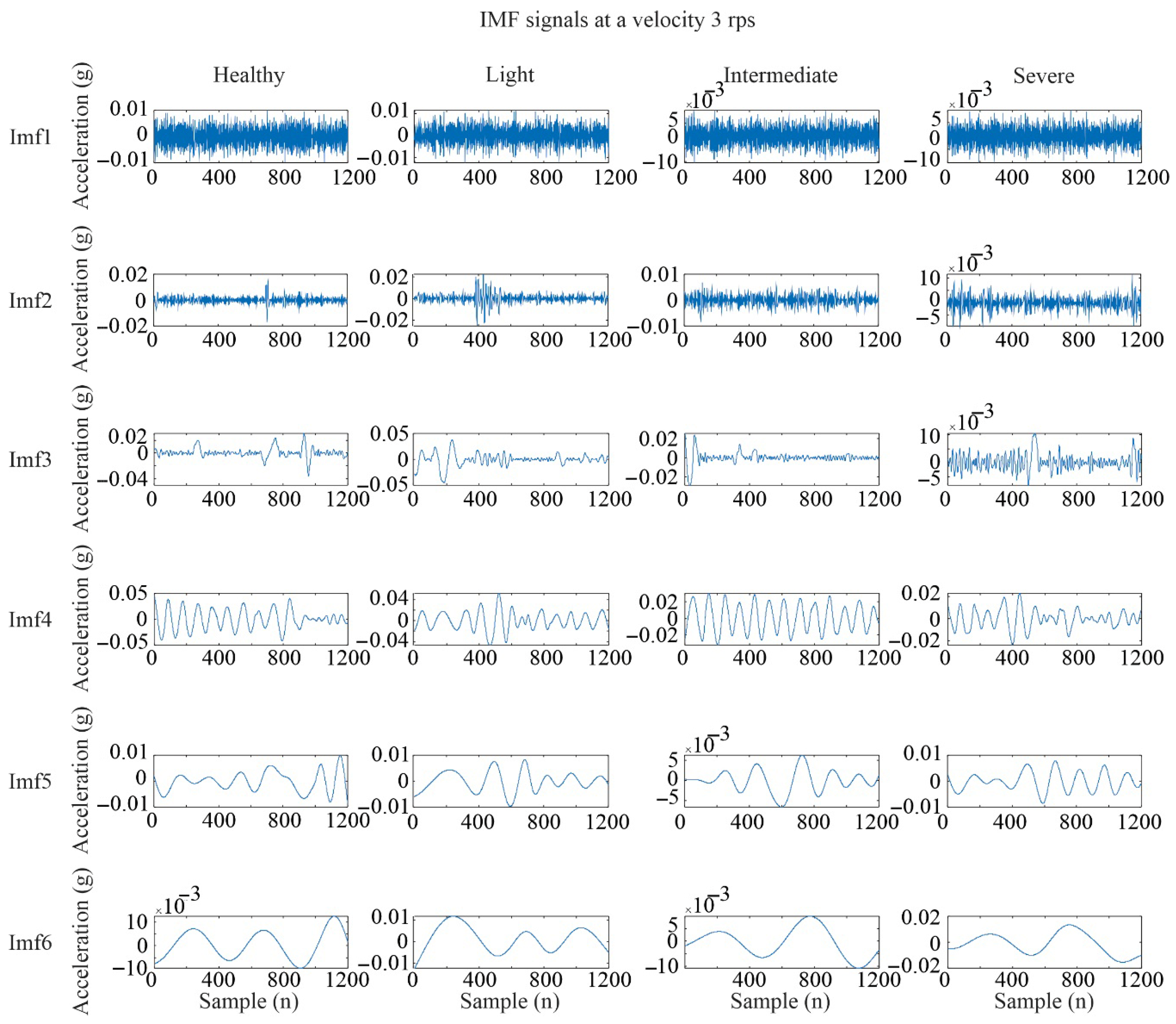
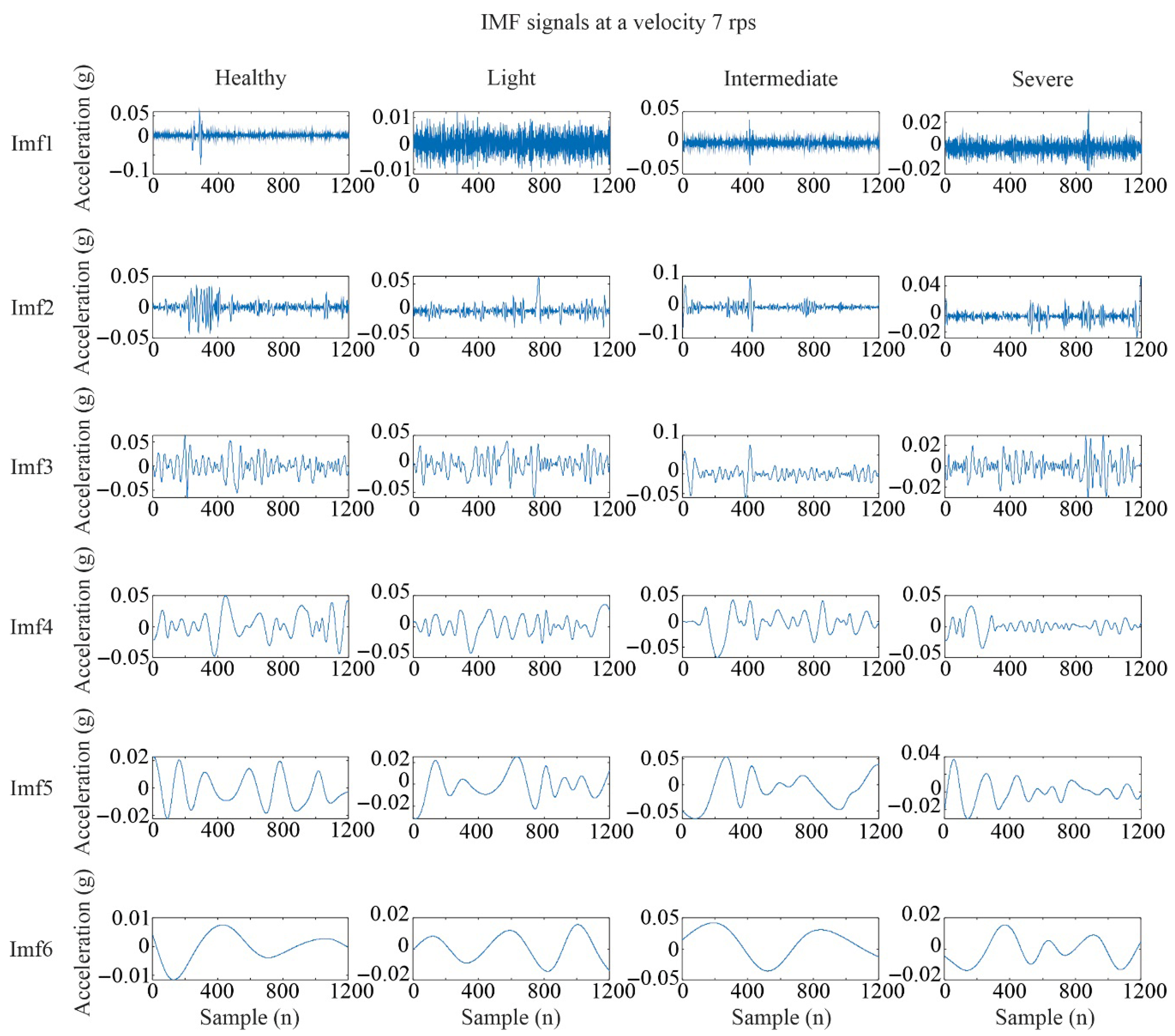
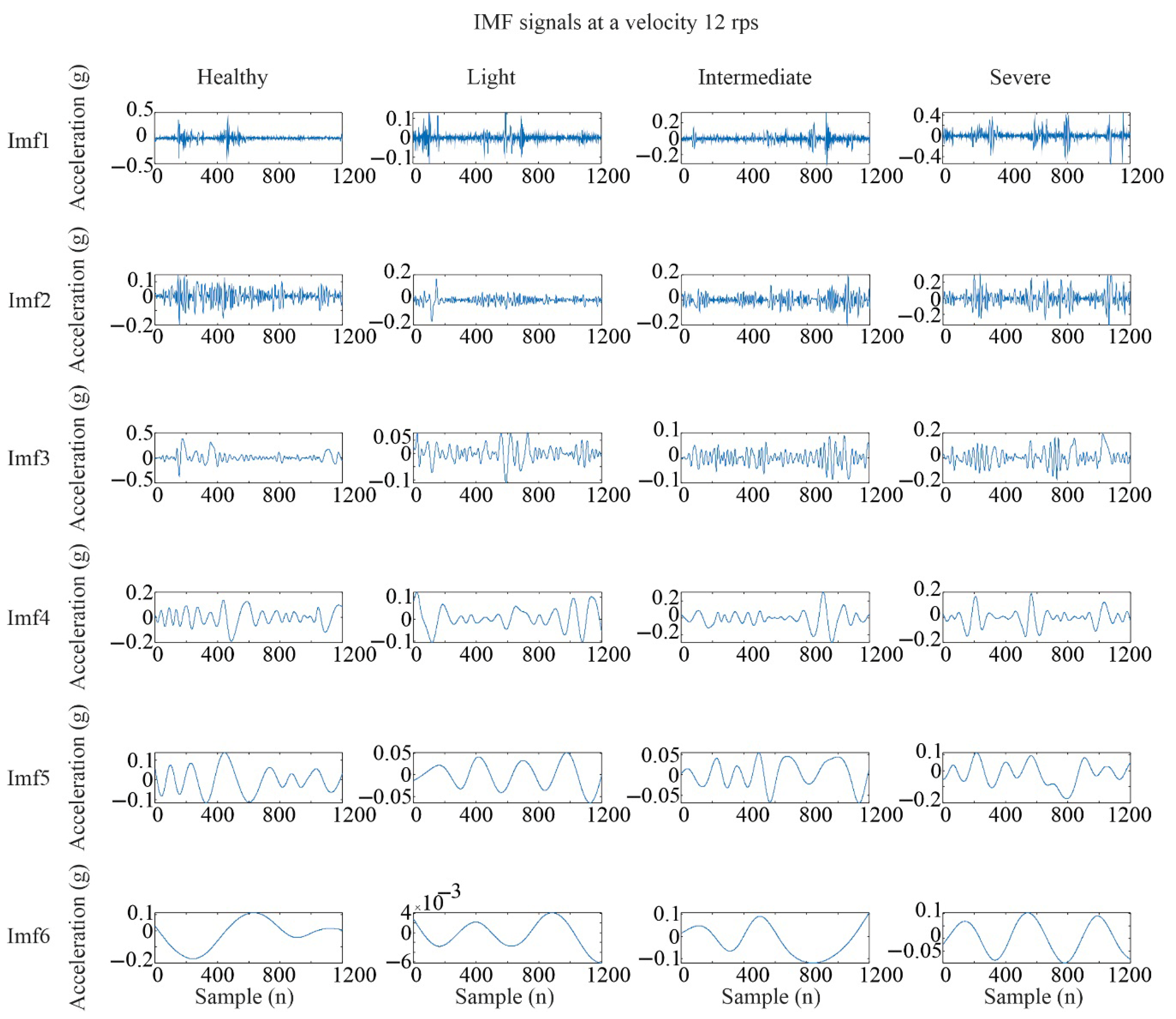
For image generation, the EMD algorithm was applied to each vibration signal, producing six IMFs per signal. Figure 6, Figure 7 and Figure 8 present a comparison of the IMFs obtained for the four blade conditions across the three rotational speed levels. Although in some cases more IMFs were obtained, a full analysis of the entire dataset revealed that six IMFs were sufficient to capture the relevant signal characteristics for all conditions. To avoid excessive plots, only the results from the Y axis are shown, as this axis yielded the best classification performance, as will be discussed later.

To construct the images, the IMFs corresponding to each condition were arranged side by side, forming a single composite image per case. Unlike traditional approaches that use only a single IMF, this method leverages multiple IMFs to generate a more comprehensive image representation of the vibration signal. Although the same procedure was applied to all three axes, only the results for the Y axis are shown, as it has yielded better results in previous studies [6]. Figure 9 displays the resulting images for all damage conditions at each speed for the Y axis, using the IMFs shown in Figure 6, Figure 7 and Figure 8. As a result, a total of 12,000 images at a resolution of 512 × 512 pixels were generated for each wind turbine angular speed level. The chosen resolution follows the criteria adopted in previous studies; nevertheless, further analyses using alternative image dimensions are included later in this work. Once the image datasets were constructed for each axis and speed, each set was classified using a baseline CNN configuration (to be detailed in a later section), with the goal of identifying the most informative axis and reducing the volume of data to be processed. The results showed that the Y axis provided the highest classification accuracy, achieving 99% compared to 96% for the X axis and 90% for the Z axis.

Although the Y axis already yielded excellent classification results, the next step involved testing different CNN parameters to determine whether the complexity of the baseline CNN could be reduced without compromising accuracy. This included evaluating different input image sizes and CNN configurations to achieve a more efficient model.

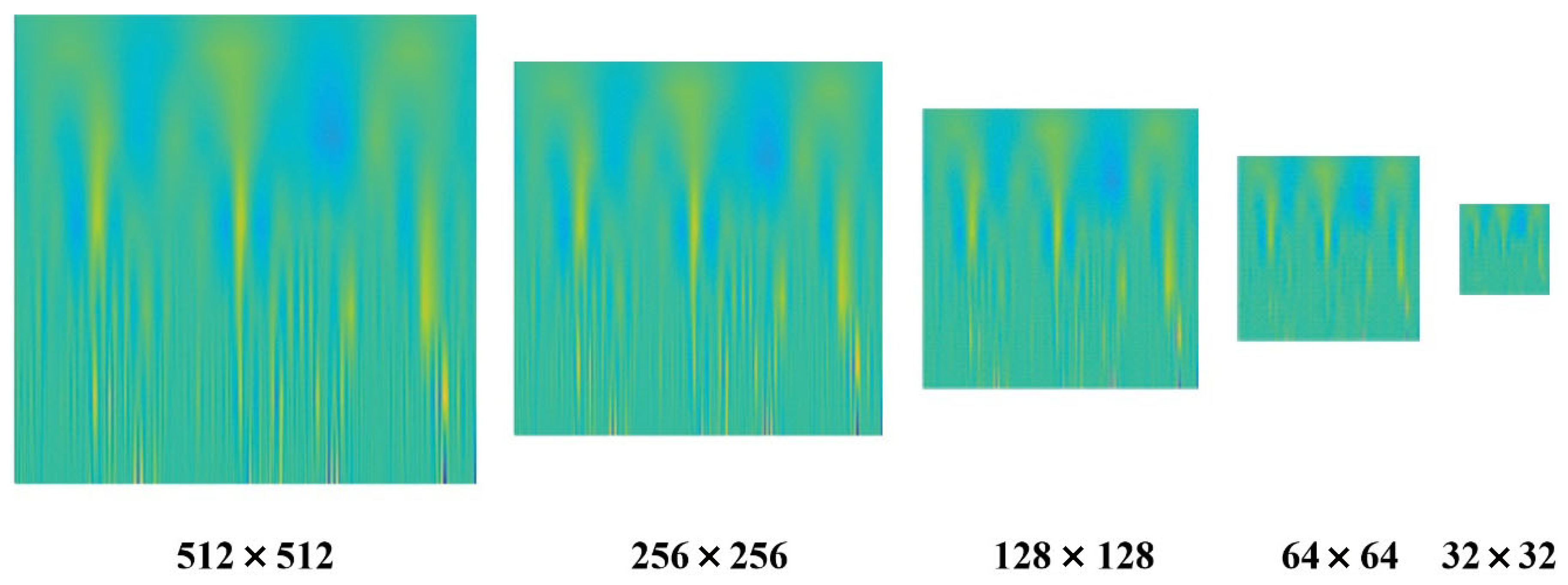
Once the most representative axis was selected, different image sizes were tested to reduce computational load while maintaining high classification accuracy. While smaller image sizes reduce the number of operations required, they may also cause loss of important features. At this stage, only the images from the Y axis were analyzed, resulting in 4000 images per rotational speed (see Table 1). Figure 10 illustrates the different image sizes evaluated in this work for the case of severe damage: 512 × 512, 256 × 256, 128 × 128, 64 × 64, and 32 × 32 pixels. The 128 × 128 resolution was selected as a suitable trade-off between image size and classification efficiency. Although larger image sizes do tend to preserve more detail and may lead to slightly improved classification accuracy, increasing image resolution significantly raises computational complexity, both in terms of memory requirements and processing time. This may hinder real-time implementation or deployment of low-power embedded systems. On the other hand, smaller image sizes offer the advantage of reduced computational load during training and inference, which is advantageous for microcontroller-based implementations. However, when the resolution is significantly reduced, important details may be lost due to pixel compaction, which can negatively impact performance.

4.3. Convolutional Neural Network

As previously mentioned, a total of 4000 images were used per axis. For this study, a static 60-20-20 split was employed, allocating 2400 images for training (60%), 800 for testing (20%), and 800 for validation (20%). This approach was adopted for the initial evaluation of the model due to its simplicity and reproducibility, also ensuring consistent class distribution across splits and enabling fair model evaluation and reproducible comparisons during architecture tuning; this is particularly important given the limited dataset size, which is relatively small for deep learning approaches such as CNNs. Future research will explore more robust validation strategies and include data from varied operating conditions to enhance and assess model generalizability.

The initial learning rate was set to 0.001, the maximum number of epochs to 4, and the mini-batch size to 50. Although these parameters were chosen empirically, they represent a reasonable starting point, as they are commonly used in similar classification tasks and help ensure stable convergence during training. After defining these training parameters, various CNN architectures were tested by varying the number of convolutional layers, the number of filters, and the filter sizes. 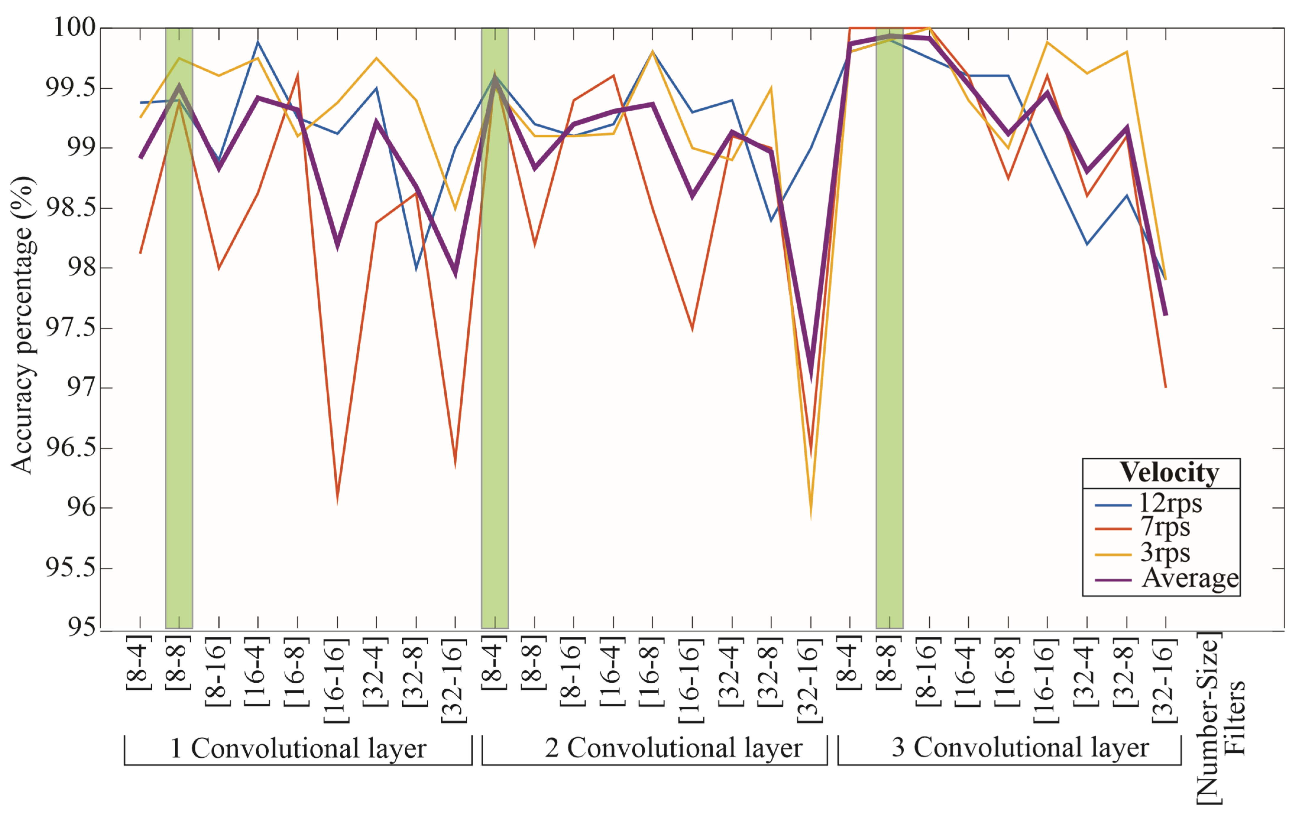Figure 11 presents the classification accuracy obtained with the different CNN configurations, considering combinations of filter numbers (i.e., 8, 16, and 32), filter sizes (i.e., 4, 8, and 16), and convolutional layers (i.e., one, two, and three layers). The best configuration for each layer count is highlighted with a green rectangle, based on the average accuracy obtained across all rotational speeds, which is indicated by the purple line.

Although no automated optimization algorithm was employed, the systematic evaluation of multiple configurations provides a comprehensive understanding of the architecture’s performance behavior. Furthermore, the selected values for the number and size of filters are widely used in lightweight CNN designs, making them suitable for exploring the trade-off between complexity and accuracy.

Although the results indicate that the configuration with three convolutional layers achieves the highest accuracy, it also entails a significantly higher computational cost. Therefore, a configuration with a single convolutional layer using eight filters of size 8 × 8 was selected as a compromise between classification performance and computational efficiency. This final architecture receives input images of size 128×128, applies a single convolutional layer followed by a max pooling operation, and uses the ReLU activation function to introduce nonlinearity. The output layer consists of four neurons, each corresponding to one of the defined classes. The final selected architecture is illustrated in Figure 12. Nevertheless, the other configurations remain valid alternatives in scenarios where maximizing accuracy is the primary objective.

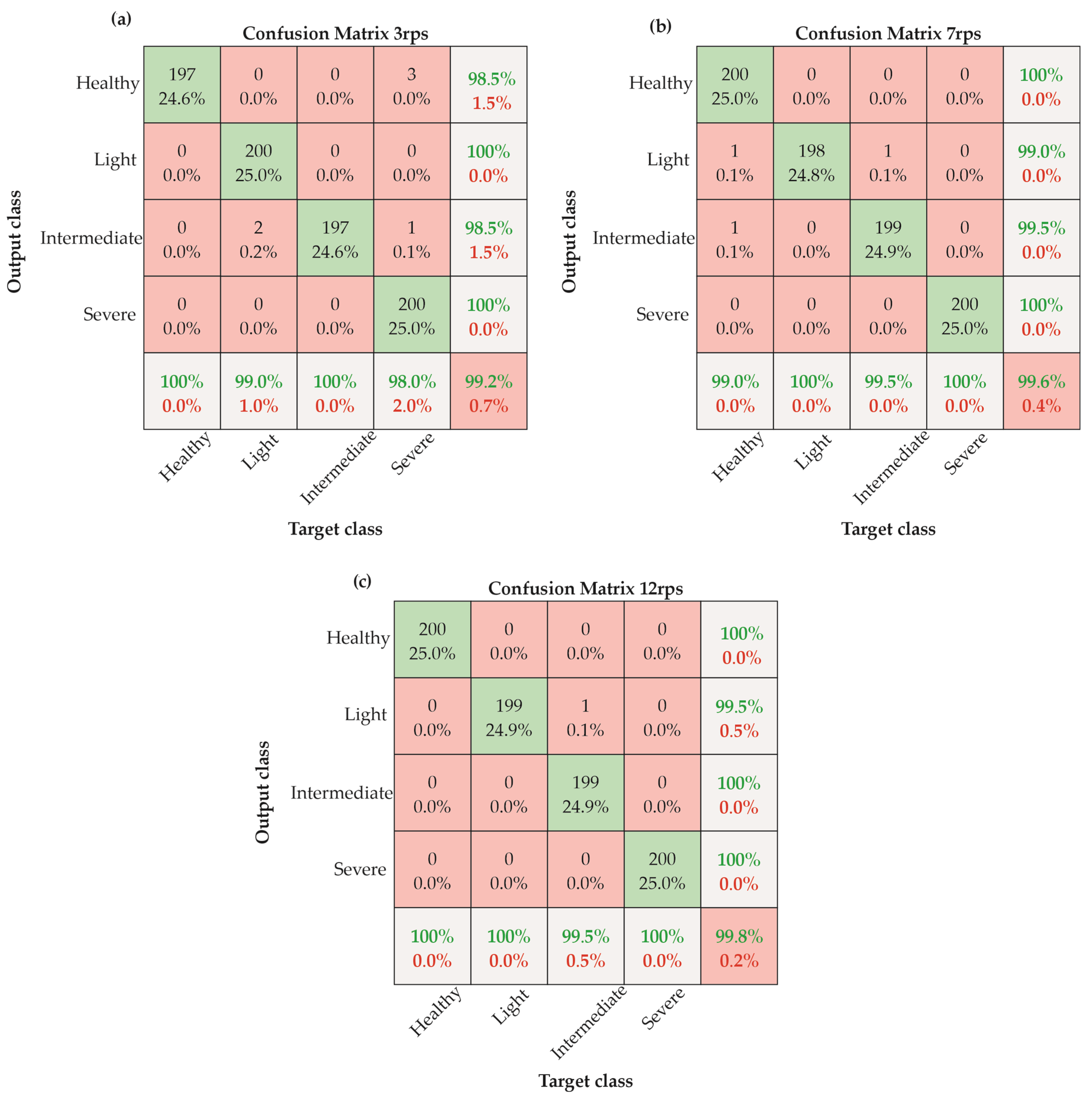
The final CNN configuration was applied to the different rotational speed levels considered in this study, yielding high classification performance. Figure 13 presents the confusion matrices obtained using the selected architecture, with classification accuracies of 99.2%, 99.6%, and 99.8% for 3 rps, 7 rps, and 12 rps, respectively. These results correspond to an average accuracy of 99.5% across all conditions.

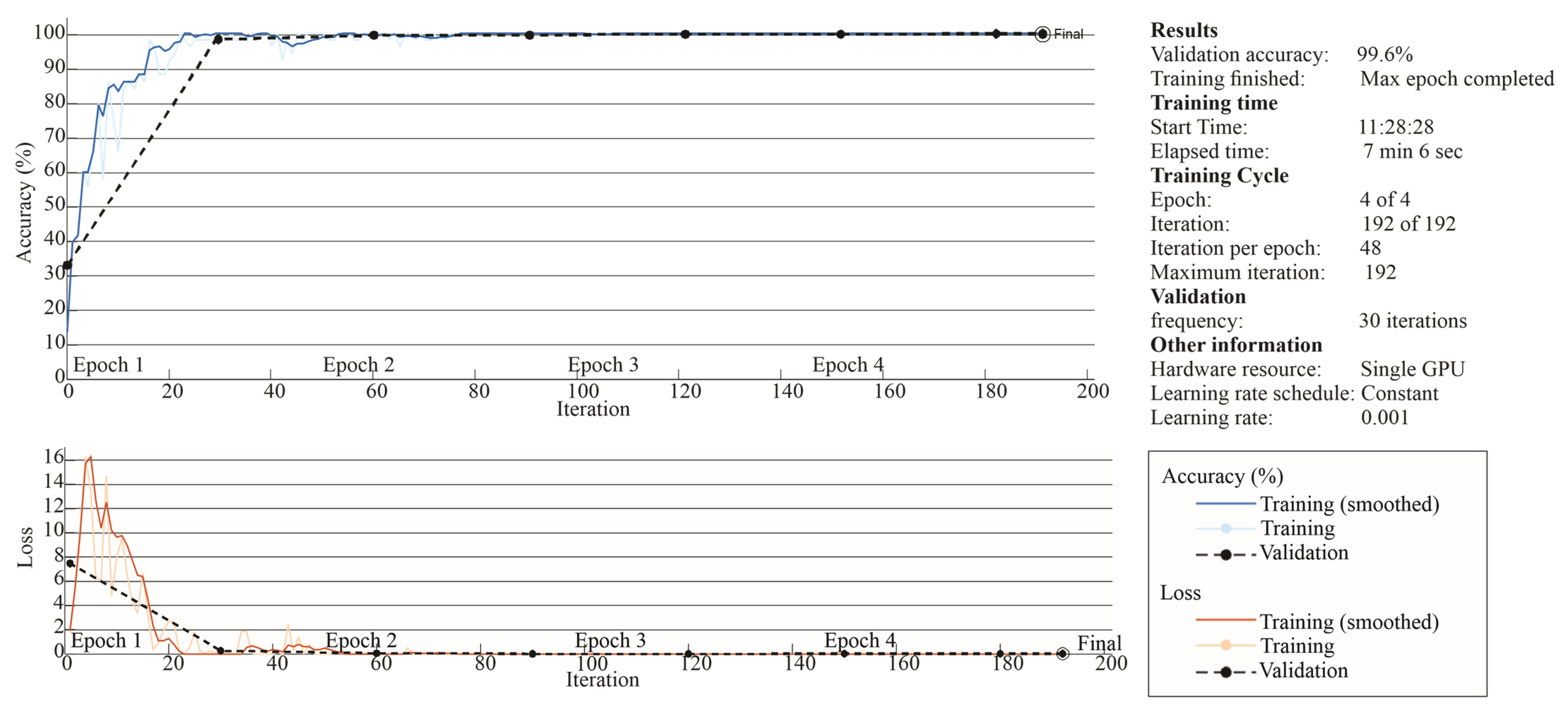
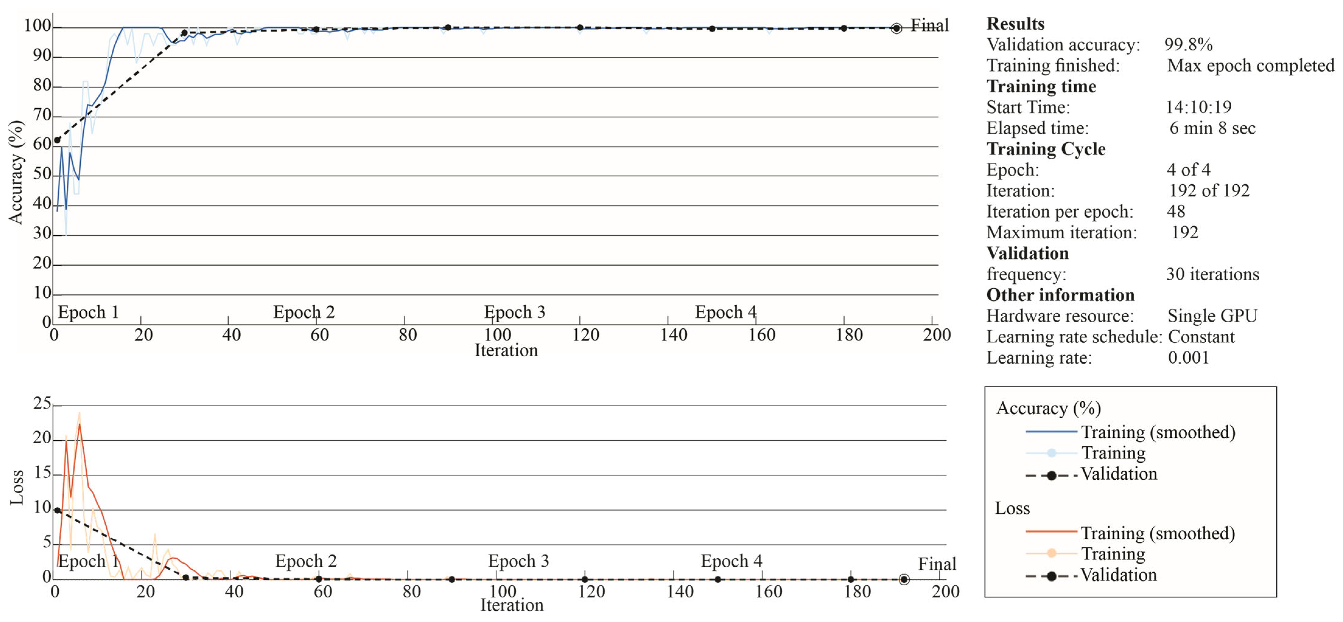
Figure 14, Figure 15 and Figure 16 show the corresponding accuracy and loss curves for each rotational speed level. The loss corresponds to the categorical cross-entropy function, which is commonly used for multi-class classification problems due to its ability to penalize incorrect class predictions more effectively. Additionally, the optimization process was carried out using the ADAM optimizer, which combines the advantages of both AdaGrad and RMSProp, allowing efficient and stable convergence during training.

The classification performance remained consistently high across the three tested rotational speeds: 99.2% at 3 rps, 99.6% at 7 rps, and 99.8% at 12 rps (see Figure 14, Figure 15 and Figure 16, respectively). These results confirm the robustness of the proposed method under varying operating conditions. Notably, accuracy exceeded 90% between epochs 20 and 40 for all cases, indicating rapid convergence and suggesting that the input data provide sufficient variability to allow clear class separation. Moreover, both the accuracy and loss curves stabilized as early as epochs 3 to 4, implying that the model required minimal training to achieve its final performance.

5. Discussion

Table 2. Comparison of the proposed work with similar works.

Work	Methodology	Signal	Number of Severity/Wind Velocity	Automatic Detection	Accuracy
[6]	Statistical indicators and machine learning	Vibrations	3/3	No	96%
[20]	Optical time domain reflectometry and Optical frequency domain reflectometry	Strain profiles	1/--	No	--
[21]	K-nearest neighbor and fractal dimension	Noise signals	1/1	No	98.9%
[22]	Unmanned aerial vehicles, Haar-like features, and logitboost, decision tree, and support vector machine	UAV images	--	Yes	--
[24]	Convolutional neural network, acoustic signals, and short time Fourier transform spectrograms	Acoustic	--	Yes	97.11%
[25]	Drone inspection images and convolutional neural network	Drone inspection images	4/1	Yes	81.1%
[28]	Ensemble Empirical Mode Decomposition, Videogrammetry, and finite element model	Videogrammetry Vibration	--	No	~95.75%
Proposed work	Empirical mode decomposition and convolutional neural network	Vibrations	3/3	Yes	~99.5%

presents a comparison between the proposed approach and several related works from the literature. The table includes the methodology used, the type of signal analyzed [6,28], the number of damage severity levels considered, the rotational speed conditions applied, whether feature extraction is performed automatically, and the classification accuracy reported in each study.

Among the reviewed works, vibration signals appear as the most commonly used data source, given their ability to capture informative patterns related to structural integrity [6,28]. However, the way these signals are processed varies significantly. In traditional ML approaches, signal characterization often relies on manually selected statistical features [6], which are not automatically extracted and may vary depending on the application or expert knowledge. In contrast, deep learning approaches, such as the one proposed in this study, automatically learn relevant features during the training process, reducing the need for manual feature engineering.

While deep learning techniques are typically applied to image-based inputs, the origin of these images differs across studies. In some cases, images are captured using cameras mounted on UAVs [22,25], which introduces additional challenges such as camera positioning errors, increased operational costs, and the fact that image acquisition is usually performed on a scheduled basis rather than continuously. In contrast, the proposed methodology generates images directly from vibration signals obtained via fixed sensors. By leveraging stationary vibration sensors, this method offers cost-effective and continuous monitoring, enabling timelier detection of incipient faults compared to the scheduled data acquisition of UAV-based methods.

Some works have also explored alternative signals such as optical measurements using DAS or AFDR systems [17], or even noise signals analyzed with KNN and fractal-based methods [20,21]; however, these approaches often lack scalability or automatic feature detection. Although spectrograms based on the STFT are frequently used for generating input images [24], this technique can incur higher computational complexity due to fixed resolution trade-offs. Instead, EMD has been used for image generation, offering an efficient, data-driven alternative well-suited for non-stationary signals such as those produced by vibration in rotating machinery. Moreover, unlike techniques such as the Multistage Algorithm, Prony or Matrix Pencil methods, which assume linearity or require predefined model orders, the extracted IMFs do not rely on predefined model orders and signal-specific oscillatory components, which makes them particularly suitable for identifying incipient damage.

Therefore, in summary, the proposed methodology demonstrates a favorable balance between accuracy and efficiency, making it a competitive option among existing approaches, particularly in applications requiring real-time or low-cost monitoring solutions. This is achieved through the combination of vibration signal analysis, EMD, and CNN, enabling automated feature extraction and continuous monitoring, thereby addressing limitations associated with methods relying on costly UAV inspections or manual feature engineering. Furthermore, the method was validated under multiple rotational speeds and four levels of damage severity, demonstrating high classification accuracy and consistent performance across varying operational conditions. To further enhance its practical application, future research will focus on scalability to larger turbines. While this study demonstrates the efficacy of the proposed methodology on a low-power turbine, scalability to larger turbines poses unique challenges. Increased turbine size correlates with greater vibration signal complexity, potentially necessitating more sensitive sensors and sophisticated CNN architectures. Future research will address these challenges by acquiring data from real-world operational environments and developing robust training techniques to ensure CNN adaptability to wind turbine speed variations and other environmental factors. Additionally, the correlation between crack position and vibration patterns will be investigated, hypothesizing that specific locations may enable crack localization for more efficient repairs. Moreover, future studies will propose fatigue-based testing and non-destructive evaluation (e.g., ultrasound or thermography) to validate severity beyond cut depth. This will further expand the contribution of the proposed methodology, potentially leading to more efficient and targeted maintenance strategies for wind turbines.

6. Conclusions

In this work, a method was developed to identify crack damage that could lead to catastrophic failures in wind turbines if not detected in time. To validate the proposed methodology, controlled damage was introduced into a blade of a low-power wind turbine. The results demonstrate that combining vibration signal images, generated using the EMD method and the first six IMFs, with CNN models enables accurate classification of blade conditions into four categories: healthy and light, intermediate, and severe damage.

Therefore, to determine the most convenient CNN training configuration, multiple architectures were evaluated under three different rotational speeds. Average classification accuracy was used as a criterion to select a configuration that offered a balanced performance across all cases. To enhance performance analysis, the architectures were grouped based on the number of convolutional layers, and the best-performing configuration within each group was selected according to its average accuracy.

A CNN architecture with a single convolutional layer and eight filters of size 8×8 achieved an average classification accuracy of 99.5% across 3 rps, 7 rps, and 12 rps. These results highlight the feasibility of an automated, low-complexity system for efficient vibration-based fault diagnosis. Although higher accuracy could be achieved by increasing network complexity, this would also raise computational costs. Even though the method was tested on a low-power wind turbine, the promising results suggest its potential scalability to larger wind turbine systems.

Future work will focus on analyzing additional fault types, including combined or compound defects, and exploring alternative optimization algorithms within deep learning to enhance diagnostic performance. One limitation of the present study is the use of fixed wind turbine angular speeds centered on steady-state conditions, which do not always reflect the variability of real-world operating environments. Additionally, the effect of crack position is another that can be studied, as it can significantly influence the dynamic response of the system and, consequently, the effectiveness of damage detection algorithms.

To further improve the practical applicability and robustness of the proposed methodology, future work will also address the following areas: implementing optimization algorithms, such as Bayesian optimization or genetic algorithms, for the automated selection of optimal CNN hyperparameters; testing the methodology on a wider range of wind turbine models, including those with different designs and power ratings, to assess its scalability and adaptability; investigating cracks with varying sizes and geometric shapes; and conducting field tests in real-world outdoor environments to evaluate the performance of the methodology under realistic operating conditions, including variable wind turbine speeds, turbulence, and environmental noise.