

Leveraging Spectral Neighborhood Information for Corn Yield Prediction with Spatial-Lagged Machine Learning Modeling: Can Neighborhood Information Outperform Vegetation Indices?

 , ,
, ,  and
and
Abstract
1. Introduction
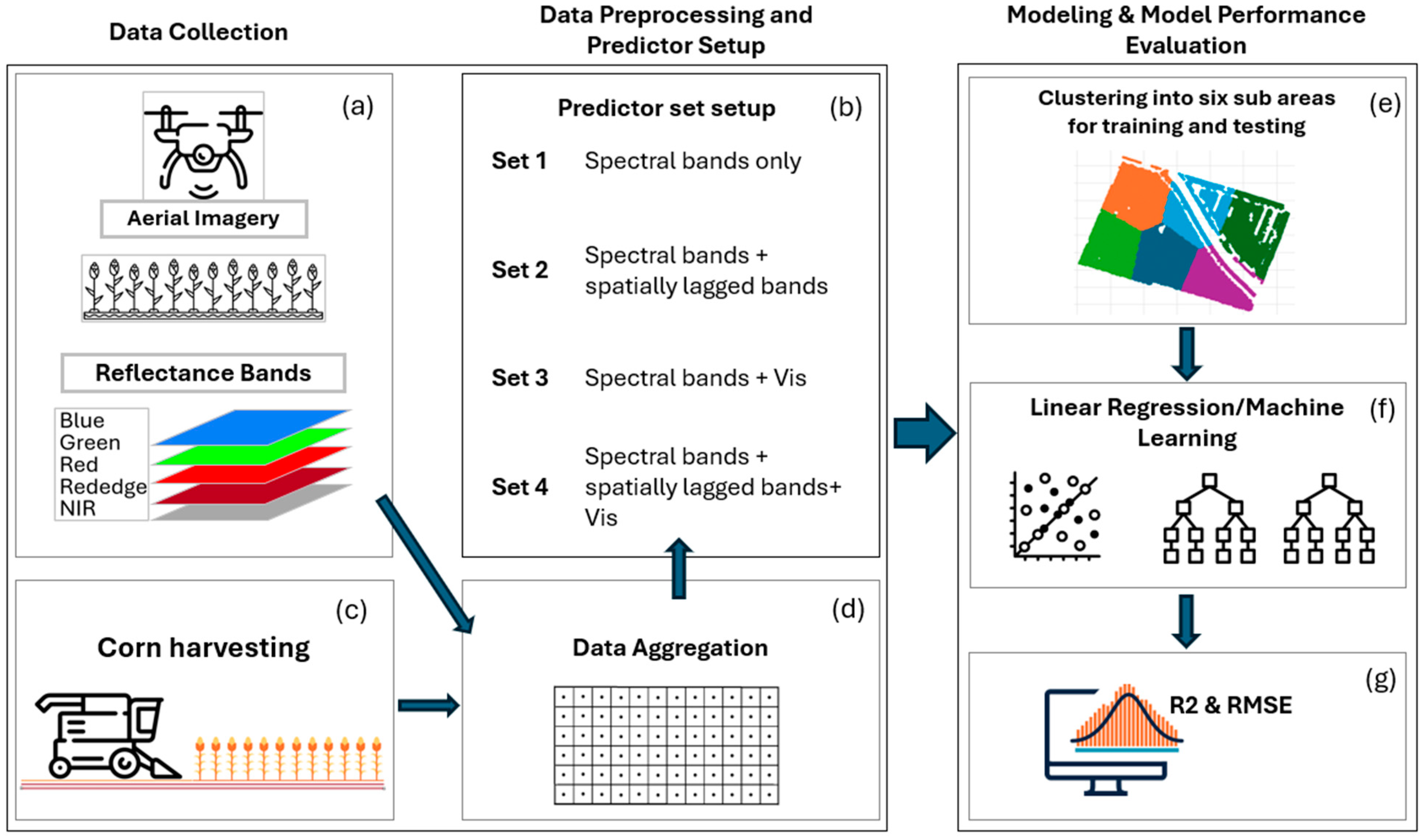
2. Methodology
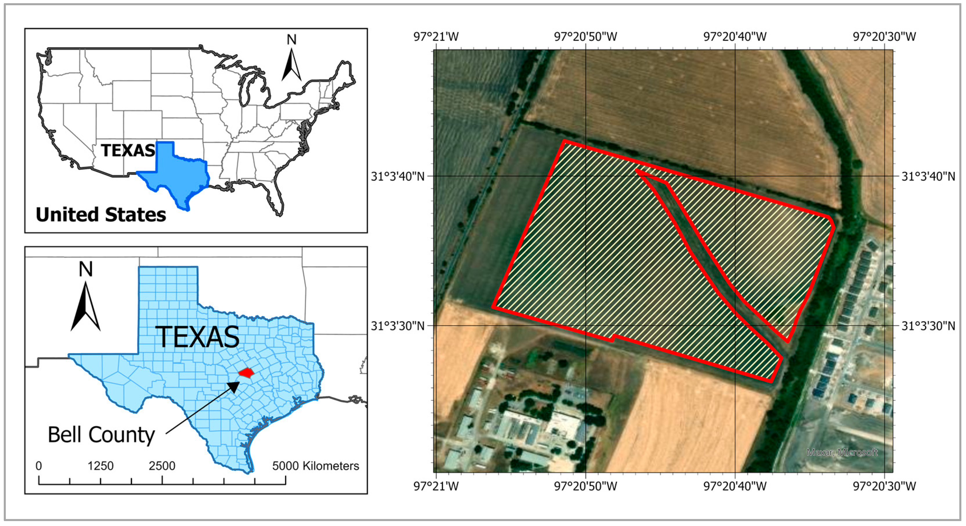
2.1. Study Area
2.2. Data Collection and Processing
2.2.1. Corn Yield Data Collection Processing
2.2.2. Imagery Processing
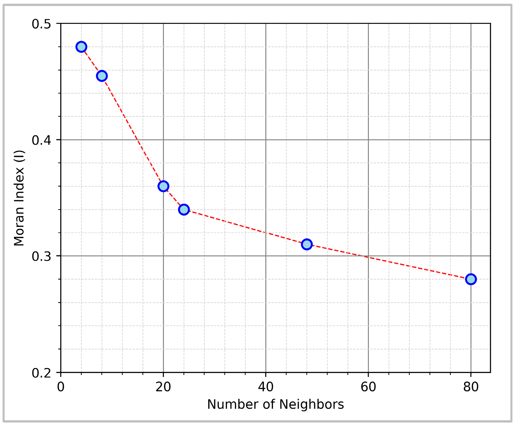
2.3. Spatial Autocorrelation Evaluation
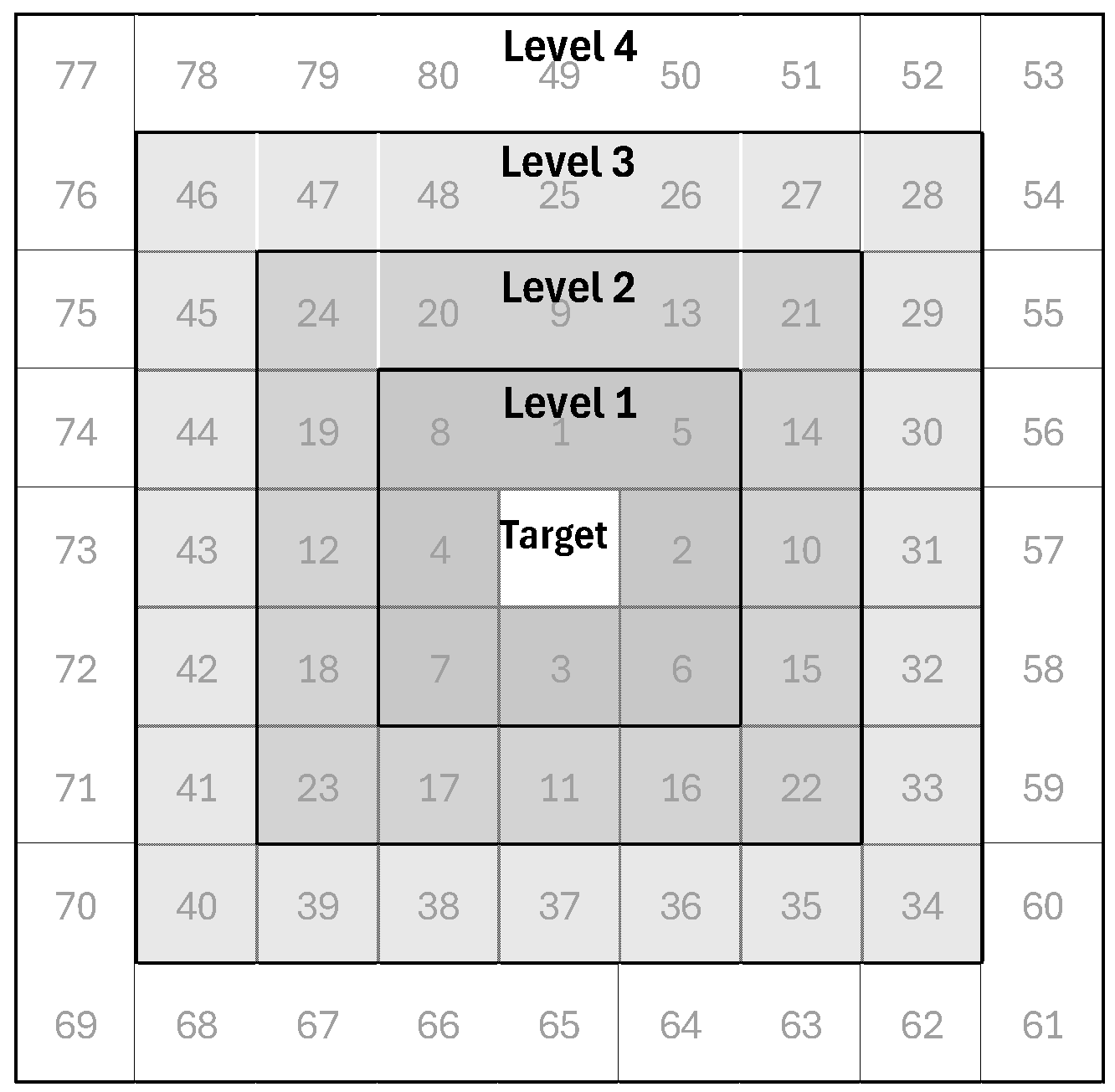
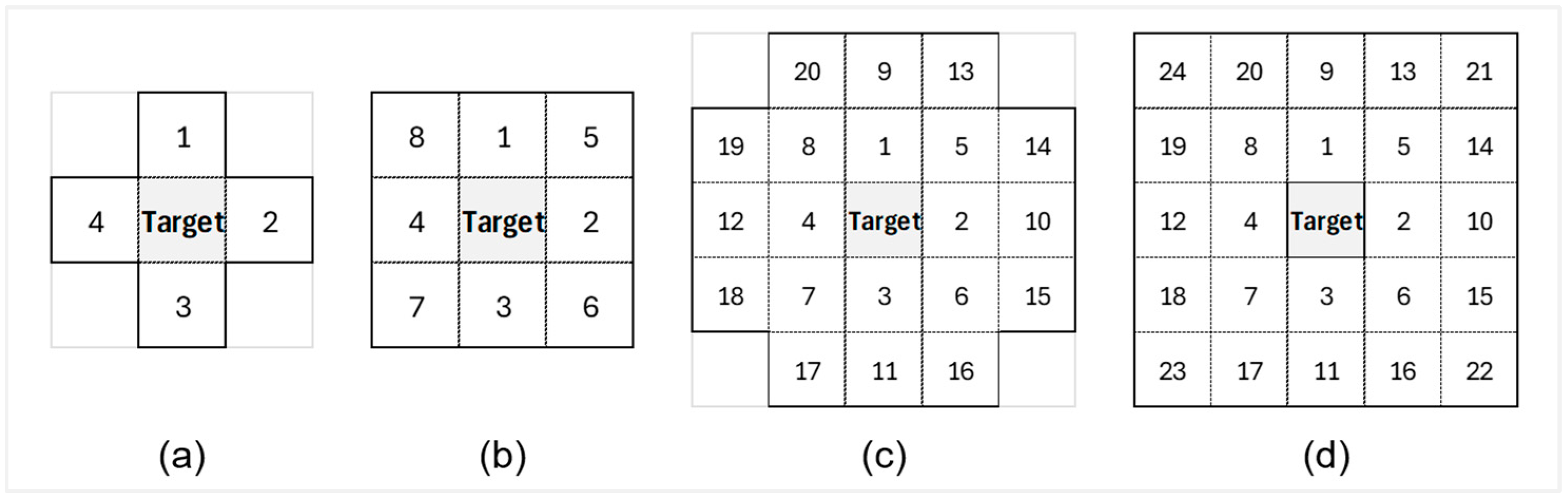
2.4. Setting up Predictor Sets for Modeling

| Vegetation Index | Name | Equation | Ref. |
|---|---|---|---|
| CREI | Chlorophyll red-edge index | [37] | |
| GCI | Green chlorophyll index | [37] | |
| NPCI | Normalized pigment chlorophyll index | [38] | |
| ARI | Anthocyanin reflectance index | [39] | |
| CCCI | Canopy chlorophyll content index | [40] | |
| EVI | Enhanced vegetation index | [41] | |
| MCARI | Modified chlorophyll absorption in reflectance index (red) | [42] | |
| MCCI | Modified chlorophyll content index | ||
| NDRE | Normalized difference red-edge index | [40] | |
| NG | Normalized green index | [43] | |
| BGI | Blue green pigment index | [44] | |
| NGRDI | Normalized green red difference index | [45] | |
| PPR | Plant pigment ratio | [46] | |
| PSRI | Plant senescence reflectance index | [47] | |
| TVI | Triangular vegetation index | [48] | |
| GNDVI | Green normalized difference vegetation index | [49] | |
| MTVI2 | Modified triangular vegetation index (TVI) 2 | [50] | |
| NDVI | Normalized difference vegetation index | [51] | |
| B-NDVI | Blue normalized difference vegetation index | [52] | |
| TCI | Triangular chlorophyl index | [50] | |
| MSAVI | Modified soil-adjusted vegetation index | [53] | |
| RDVI | Renormalized difference vegetation index | [54] | |
| SAVI | Soil-adjusted vegetation index | [41] | |
| TrVI | Transformed vegetation index | [51] | |
| TSAVI | Transformed soil-adjusted vegetation index | [55] |
2.5. Spatial Regression Modeling
2.5.1. Spatial Lag X Model (SLX)
2.5.2. Machine Learning Models
Random Forest
Extreme Gradient Boosting (XGB)
Extremely Randomized Tree Regression (ET)
Gradient Boosting Regressor (GBR)
2.6. Model Training and Testing
2.6.1. Computation Tools
2.6.2. Hyperparameter Tunning
2.7. Model Performance Evaluation
3. Results
3.1. Spatial Autocorrelation
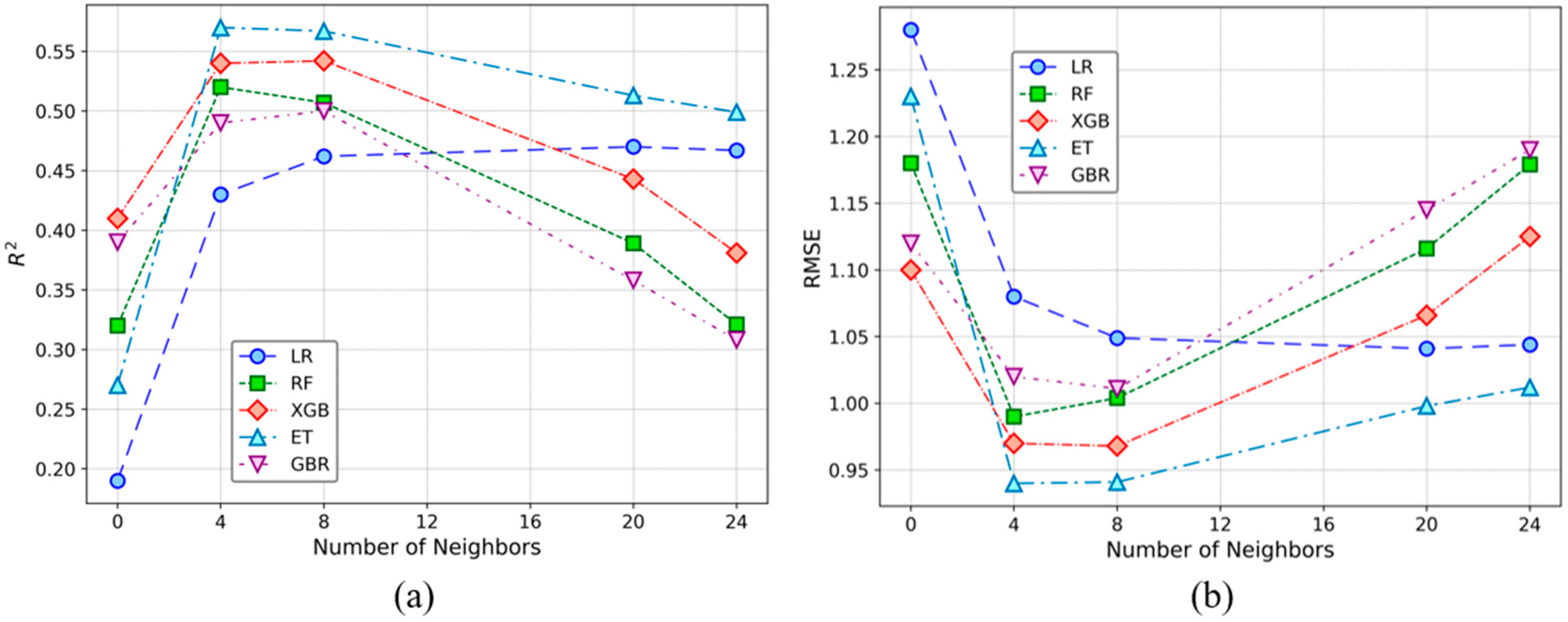
3.2. Model Performance With and Without Neighbor Information
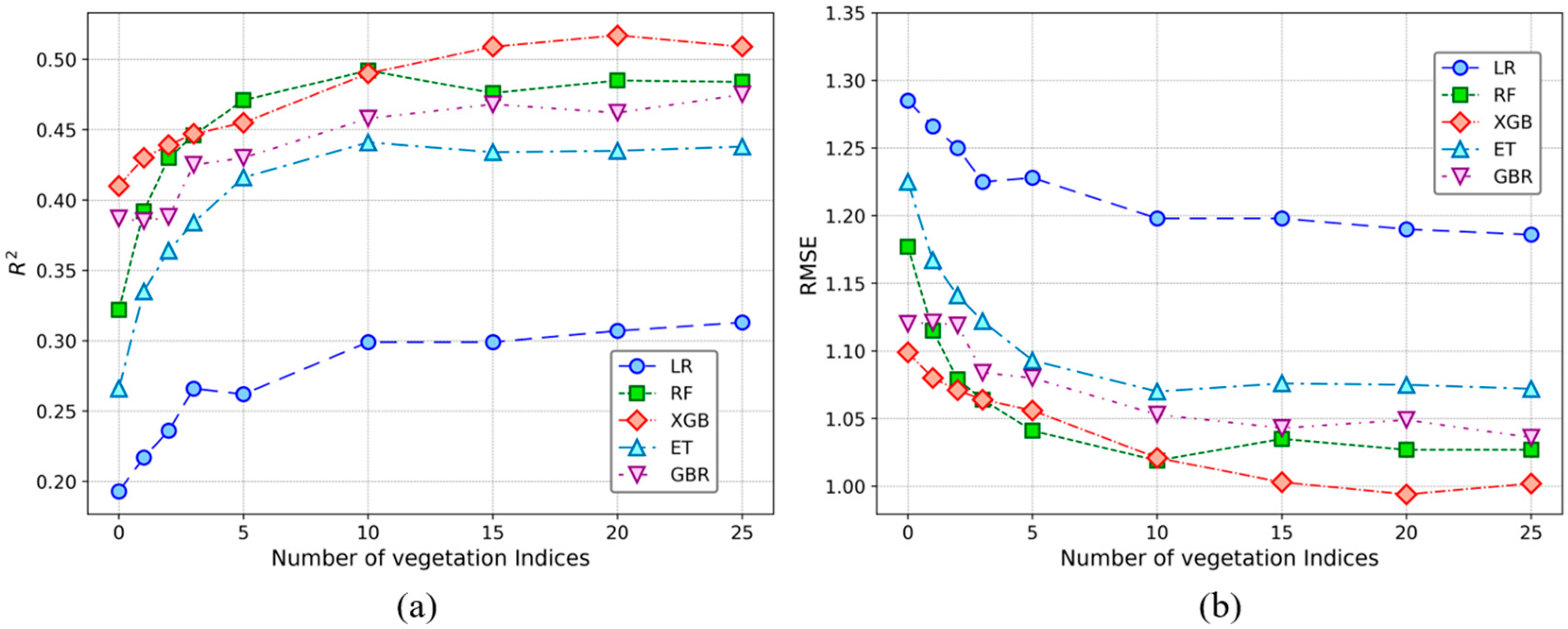
3.3. Model Performance With and Without Vegetation Indices
3.4. Model Performance Combining Neighborhood Information and Vegetation Indices
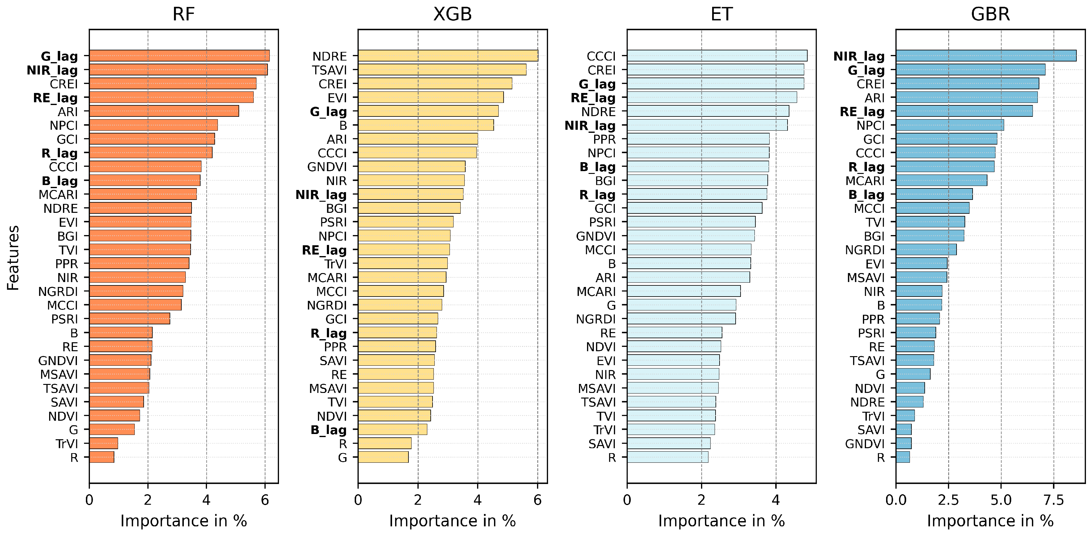
3.5. Feature Importance When Combining All the Predictors
3.6. Model Performance Comparison Across Predictor Sets
4. Discussion
4.1. Spatial Autocorrelation of Corn Yield
4.2. Neighborhood Information and Model Performance
4.3. Vegetation Indices and Model Performance
4.4. Model Performance When Combining All Predictors
4.5. Implications for Future Research
5. Conclusions
Author Contributions
Funding
Institutional Review Board Statement
Informed Consent Statement
Data Availability Statement
Acknowledgments
Conflicts of Interest
References
- Filippi, P.; Jones, E.J.; Wimalathunge, N.S.; Somarathna, P.D.S.N.; Pozza, L.E.; Ugbaje, S.U.; Jephcott, T.G.; Paterson, S.E.; Whelan, B.M.; Bishop, T.F.A. An approach to forecast grain crop yield using multi-layered, multi-farm data sets and machine learning. Precis. Agric. 2019, 20, 1015–1029. [Google Scholar] [CrossRef]
- Lobell, D.B.; Roberts, M.J.; Schlenker, W.; Braun, N.; Little, B.B.; Rejesus, R.M.; Hammer, G.L. Greater Sensitivity to Drought Accompanies Maize Yield Increase in the U.S. Midwest. Science 2014, 344, 516–519. [Google Scholar] [CrossRef] [PubMed]
- Hatfield, J.L.; Prueger, J.H. Temperature extremes: Effect on plant growth and development. Weather. Clim. Extremes 2015, 10, 4–10. [Google Scholar] [CrossRef]
- Zhou, H.; Yang, J.; Lou, W.; Sheng, L.; Li, D.; Hu, H. Improving grain yield prediction through fusion of multi-temporal spectral features and agronomic trait parameters derived from UAV imagery. Front. Plant Sci. 2023, 14, 1217448. [Google Scholar] [CrossRef]
- Noa-Yarasca, E.; Leyton, J.M.O.; Angerer, J. Biomass Time Series Forecasting Using Deep Learning Techniques. Is the Sophisticated Model Superior? In Biometry and Statistical Computing; ASA, CSSA, SSSA International Annual Meeting: St. Louis, MO, USA; Available online: https://scisoc.confex.com/scisoc/2023am/meetingapp.cgi/Paper/151648 (accessed on 10 April 2024).
- Hunt, E.R., Jr.; Hively, W.D.; Fujikawa, S.J.; Linden, D.S.; Daughtry, C.S.T.; McCarty, G.W. Acquisition of NIR-Green-Blue Digital Photographs from Unmanned Aircraft for Crop Monitoring. Remote Sens. 2010, 2, 290–305. [Google Scholar] [CrossRef]
- Cicek, H.; Sunohara, M.; Wilkes, G.; McNairn, H.; Pick, F.; Topp, E.; Lapen, D. Using vegetation indices from satellite remote sensing to assess corn and soybean response to controlled tile drainage. Agric. Water Manag. 2010, 98, 261–270. [Google Scholar] [CrossRef]
- Killeen, P.; Kiringa, I.; Yeap, T.; Branco, P. Corn Grain Yield Prediction Using UAV-Based High Spatiotemporal Resolution Imagery, Machine Learning, and Spatial Cross-Validation. Remote Sens. 2024, 16, 683. [Google Scholar] [CrossRef]
- Moeckel, T.; Dayananda, S.; Nidamanuri, R.R.; Nautiyal, S.; Hanumaiah, N.; Buerkert, A.; Wachendorf, M. Estimation of Vegetable Crop Parameter by Multi-temporal UAV-Borne Images. Remote Sens. 2018, 10, 805. [Google Scholar] [CrossRef]
- Panda, S.S.; Ames, D.P.; Panigrahi, S. Application of Vegetation Indices for Agricultural Crop Yield Prediction Using Neural Network Techniques. Remote Sens. 2010, 2, 673–696. [Google Scholar] [CrossRef]
- Lesage, J.; Pace, R.K. Introduction to Spatial Econometrics, 1st ed.; CRC Press: Boca Raton, FL, USA, 2023. [Google Scholar]
- Lou, M.; Zhang, H.; Lei, X.; Li, C.; Zang, H. Spatial Autoregressive Models for Stand Top and Stand Mean Height Relationship in Mixed Quercus mongolica Broadleaved Natural Stands of Northeast China. Forests 2016, 7, 43. [Google Scholar] [CrossRef]
- Fang, C.; Liu, H.; Li, G.; Sun, D.; Miao, Z. Estimating the Impact of Urbanization on Air Quality in China Using Spatial Regression Models. Sustainability 2015, 7, 15570–15592. [Google Scholar] [CrossRef]
- Ponciano, P.F.; Scalon, J.D. Análise espacial da produção leiteira usando um modelo autoregressivo condicional. Semin. Cienc. Agrar. 2010, 31, 487–496. [Google Scholar] [CrossRef]
- Ahn, K.-H.; Palmer, R. Regional flood frequency analysis using spatial proximity and basin characteristics: Quantile regression vs. parameter regression technique. J. Hydrol. 2016, 540, 515–526. [Google Scholar] [CrossRef]
- Yoo, J.; Ready, R. The impact of agricultural conservation easement on nearby house prices: Incorporating spatial autocorrelation and spatial heterogeneity. J. For. Econ. 2016, 25, 78–93. [Google Scholar] [CrossRef]
- Guo, L.; Zhao, C.; Zhang, H.; Chen, Y.; Linderman, M.; Zhang, Q.; Liu, Y. Comparisons of spatial and non-spatial models for predicting soil carbon content based on visible and near-infrared spectral technology. Geoderma 2017, 285, 280–292. [Google Scholar] [CrossRef]
- Auffhammer, M.; Hsiang, S.; Schlenker, W.; Sobel, A. Using Weather Data and Climate Model Output in Economic Analyses of Climate Change. Rev. Environ. Econ. Policy 2013, 7, 181–198. [Google Scholar] [CrossRef]
- Dell, M.; Jones, B.F.; Olken, B.A. What Do We Learn from the Weather? The New Climate-Economy Literature. J. Econ. Lit. 2014, 52, 740–798. [Google Scholar] [CrossRef]
- Schlenker, W.; Roberts, M.J. Nonlinear temperature effects indicate severe damages to U.S. crop yields under climate change. Proc. Natl. Acad. Sci. USA 2009, 106, 15594–15598. [Google Scholar] [CrossRef]
- Hawinkel, S.; De Meyer, S.; Maere, S. Spatial Regression Models for Field Trials: A Comparative Study and New Ideas. Front. Plant Sci. 2022, 13, 858711. [Google Scholar] [CrossRef]
- Fischer, R.J.; Rekabdarkolaee, H.M.; Joshi, D.R.; Clay, D.E.; Clay, S.A. Soybean prediction using computationally efficient Bayesian spatial regression models and satellite imagery. Agron. J. 2024, 116, 2841–2849. [Google Scholar] [CrossRef]
- Ward, M.; Gleditsch, K. Spatial Regression Models; SAGE Publications: Thousand Oaks, CA, USA, 2008. [Google Scholar] [CrossRef]
- Rüttenauer, T. Spatial Regression Models: A Systematic Comparison of Different Model Specifications Using Monte Carlo Experiments. Sociol. Methods Res. 2022, 51, 728–759. [Google Scholar] [CrossRef]
- Rehman, T.H.; Lundy, M.E.; Linquist, B.A. Comparative Sensitivity of Vegetation Indices Measured via Proximal and Aerial Sensors for Assessing N Status and Predicting Grain Yield in Rice Cropping Systems. Remote Sens. 2022, 14, 2770. [Google Scholar] [CrossRef]
- Sarkar, S.; Leyton, J.M.O.; Noa-Yarasca, E.; Adhikari, K.; Hajda, C.B.; Smith, D.R. Integrating Remote Sensing and Soil Features for Enhanced Machine Learning-Based Corn Yield Prediction in the Southern US. Sensors 2025, 25, 543. [Google Scholar] [CrossRef] [PubMed]
- Effrosynidis, D.; Sylaios, G.; Arampatzis, A. The Effect of Training Data Size on Disaster Classification from Twitter. Information 2024, 15, 393. [Google Scholar] [CrossRef]
- Awan, F.M.; Saleem, Y.; Minerva, R.; Crespi, N. A Comparative Analysis of Machine/Deep Learning Models for Parking Space Availability Prediction. Sensors 2020, 20, 322. [Google Scholar] [CrossRef]
- Noa-Yarasca, E.; Leyton, J.M.O.; Angerer, J.P. Deep Learning Model Effectiveness in Forecasting Limited-Size Aboveground Vegetation Biomass Time Series: Kenyan Grasslands Case Study. Agronomy 2024, 14, 349. [Google Scholar] [CrossRef]
- Soil Survey Staff. Keys to Soil Taxonomy 11th Edition. Washington, DC, USA. Available online: https://www.nrcs.usda.gov/sites/default/files/2022-09/Keys-to-Soil-Taxonomy.pdf (accessed on 10 December 2024).
- Adhikari, K.; Smith, D.R.; Hajda, C.; Kharel, T.P. Within-field yield stability and gross margin variations across corn fields and implications for precision conservation. Precis. Agric. 2023, 24, 1401–1416. [Google Scholar] [CrossRef]
- FAO. Faostat: Crops and Livestock Products. Food and Agriculture Organization of the United Nations. Available online: https://www.fao.org/faostat/en/#data/QV (accessed on 19 July 2024).
- USDA-NASS. Quick Stats. United States Department of Agriculture, National Agricultural Statistics Service. Available online: https://quickstats.nass.usda.gov/ (accessed on 19 July 2024).
- Fu, W.J.; Jiang, P.K.; Zhou, G.M.; Zhao, K.L. Using Moran’s I and GIS to study the spatial pattern of forest litter carbon density in a subtropical region of southeastern China. Biogeosciences 2014, 11, 2401–2409. [Google Scholar] [CrossRef]
- O’sullivan, D.; Unwin, D. Geographic Information Analysis, 2nd ed.; John Wiley & Sons, Inc.: Hoboken, NJ, USA, 2010. [Google Scholar]
- Noa-Yarasca, E. A Machine Learning Model of Riparian Vegetation Attenuated Stream Temperatures. Oregon State University, Corvallis, OR, USA. Available online: https://ir.library.oregonstate.edu/downloads/0r967b65c#page=137 (accessed on 10 April 2024).
- Gitelson, A.A.; Viña, A.; Arkebauer, T.J.; Rundquist, D.C.; Keydan, G.; Leavitt, B. Remote estimation of leaf area index and green leaf biomass in maize canopies. Geophys. Res. Lett. 2003, 30, 1248. [Google Scholar] [CrossRef]
- Peñuelas, J.; Gamon, J.; Fredeen, A.; Merino, J.; Field, C. Reflectance indices associated with physiological changes in nitrogen- and water-limited sunflower leaves. Remote Sens. Environ. 1994, 48, 135–146. [Google Scholar] [CrossRef]
- Gitelson, A.A.; Merzlyak, M.N.; Zur, Y.; Stark, R.; Gritz, U. Non-Destructive and Remote Sensing Techniques for Estimation of Vegetation Status. Papers in Natural Resources, no. 273. 2001. Available online: https://digitalcommons.unl.edu/natrespapers/273/ (accessed on 18 November 2024).
- Barnes, E.M.; Clarke, T.R.; Richards, S.E.; Colaizzi, P.D.; Haberland, J.; Kostrzewski, M.; Moran, M.S. Coincident Detection of Crop Water Stress, Nitrogen Status and Canopy Density Using Ground-Based Multi-spectral Data. In Proceedings of the 5th International Conference on Precision Agriculture, Bloomington, MN, USA, 16–19 July 2000; Robert, P.C., Rust, R.H., Larson, W.E., Eds.; [Google Scholar]
- Huete, A.; Didan, K.; Miura, T.; Rodriguez, E.P.; Gao, X.; Ferreira, L.G. Overview of the radiometric and biophysical performance of the MODIS vegetation indices. Remote Sens. Environ. 2002, 83, 195–213. [Google Scholar] [CrossRef]
- Daughtry, C.S.T.; Walthall, C.L.; Kim, M.S.; De Colstoun, E.B.; McMurtrey, J.E., III. Estimating Corn Leaf Chlorophyll Concentration from Leaf and Canopy Reflectance. Remote Sens. Environ. 2000, 74, 229–239. [Google Scholar] [CrossRef]
- Marcial-Pablo, M.d.J.; Gonzalez-Sanchez, A.; Jimenez-Jimenez, S.I.; Ontiveros-Capurata, R.E.; Ojeda-Bustamante, W. Estimation of vegetation fraction using RGB and multispectral images from UAV. Int. J. Remote Sens. 2019, 40, 420–438. [Google Scholar] [CrossRef]
- Zarco-Tejada, P.J.; Berjón, A.; López-Lozano, R.; Miller, J.R.; Martín, P.; Cachorro, V.; González, M.R.; De Frutos, A. Assessing vineyard condition with hyperspectral indices: Leaf and canopy reflectance simulation in a row-structured discontinuous canopy. Remote Sens. Environ. 2005, 99, 271–287. [Google Scholar] [CrossRef]
- Tucker, C.J. Red and photographic infrared linear combinations for monitoring vegetation. Remote Sens. Environ. 1979, 8, 127–150. [Google Scholar] [CrossRef]
- Metternicht, G. Vegetation indices derived from high-resolution airborne videography for precision crop management. Int. J. Remote Sens. 2003, 24, 2855–2877. [Google Scholar] [CrossRef]
- Merzlyak, M.N.; Gitelson, A.A.; Chivkunova, O.B.; Rakitin, V.Y. Non-destructive optical detection of pigment changes during leaf senescence and fruit ripening. Physiol. Plant. 1999, 106, 135–141. [Google Scholar] [CrossRef]
- Broge, N.H.; Leblanc, E. Comparing prediction power and stability of broadband and hyperspectral vegetation indices for estimation of green leaf area index and canopy chlorophyll density. Remote Sens. Environ. 2001, 76, 156–172. [Google Scholar] [CrossRef]
- Gitelson, A.A.; Kaufman, Y.J.; Merzlyak, M.N. Use of a green channel in remote sensing of global vegetation from EOS-MODIS. Remote Sens. Environ. 1996, 58, 289–298. [Google Scholar] [CrossRef]
- Haboudane, D.; Tremblay, N.; Miller, J.R.; Vigneault, P. Remote Estimation of Crop Chlorophyll Content Using Spectral Indices Derived from Hyperspectral Data. IEEE Trans. Geosci. Remote Sens. 2008, 46, 423–437. [Google Scholar] [CrossRef]
- Rouse, J.W., Jr.; Haas, R.H.; Schell, J.A.; Deering, D.W. Monitoring Vegetation Systems in the Great Plains with Erts. 1974. Washington, DC, USA. Available online: https://ui.adsabs.harvard.edu/abs/1974NASSP.351.309R/abstract (accessed on 18 November 2024).
- Yang, C.; Everitt, J.H.; Bradford, J.M.; Murden, D. Airborne Hyperspectral Imagery and Yield Monitor Data for Mapping Cotton Yield Variability. Precis. Agric. 2004, 5, 445–461. [Google Scholar] [CrossRef]
- Qi, J.; Chehbouni, A.; Huete, A.R.; Kerr, Y.H.; Sorooshian, S. A modified soil adjusted vegetation index. Remote Sens. Environ. 1994, 48, 119–126. [Google Scholar] [CrossRef]
- Zhang, L.; Zhang, H.; Niu, Y.; Han, W. Mapping Maize Water Stress Based on UAV Multispectral Remote Sensing. Remote Sens. 2019, 11, 605. [Google Scholar] [CrossRef]
- Baret, F.; Guyot, G.; Major, D. TSAVI: A Vegetation Index Which Minimizes Soil Brightness Effects On LAI And APAR Estimation. In Proceedings of the 12th Canadian Symposium on Remote Sensing Geoscience and Remote Sensing Symposium, Vancouver, BC, Canada, 10–14 July 1989; Institute of Electrical and Electronics Engineers (IEEE): Vancouver, BC, Canada, 1989; pp. 1355–1358. [Google Scholar] [CrossRef]
- Breiman, L. Random forests. Mach. Learn. 2001, 45, 5–32. [Google Scholar] [CrossRef]
- Chen, T.; Guestrin, C. “XGBoost”. In Proceedings of the 22nd ACM SIGKDD International Conference on Knowledge Discovery and Data Mining, San Francisco, CA, USA, 13–17 August 2016; ACM: New York, NY, USA, 2016; pp. 785–794. [Google Scholar] [CrossRef]
- Geurts, P.; Ernst, D.; Wehenkel, L. Extremely randomized trees. Mach. Learn. 2006, 63, 3–42. [Google Scholar] [CrossRef]
- Natekin, A.; Knoll, A. Gradient boosting machines, a tutorial. Front. Neurorobotics 2013, 7, 21. [Google Scholar] [CrossRef]
- Friedman, J.H. Greedy function approximation: A gradient boosting machine. Ann. Stat. 2001, 29, 1189–1232. [Google Scholar] [CrossRef]
- Zhang, Z.; Zhao, Y.; Canes, A.; Steinberg, D.; Lyashevska, O. Predictive analytics with gradient boosting in clinical medicine. Ann. Transl. Med. 2019, 7, 152. [Google Scholar] [CrossRef]
- Harris, C.R.; Millman, K.J.; van der Walt, S.J.; Gommers, R.; Virtanen, P.; Cournapeau, D.; Wieser, E.; Taylor, J.; Berg, S.; Smith, N.J.; et al. Array Programming with NumPy. Nature 2020, 585, 357–362. [Google Scholar] [CrossRef]
- McKinney, W. Data Structures for Statistical Computing in Python. In Proceedings of the 9th Python in Science Conference, Austin, TX, USA, 28 June–3 July 2010; pp. 51–56. [Google Scholar]
- Pedregosa, F.; Varoquaux, G.; Gramfort, A.; Michel, V.; Thirion, B.; Grisel, O.; Blondel, M.; Prettenhofer, P.; Weiss, R.; Dubourg, V.; et al. Scikit-Learn: Machine Learning in Python. J. Mach. Learn. Res. 2011, 12, 2825–2830. [Google Scholar]
- Van Rossum, G.; Drake, F.L. Python 3 Reference Manual; CreateSpace: Scotts Valley, CA, USA, 2009. [Google Scholar]
- Grossfeld, B. Geography and law. Mich. Law Rev. 1984, 82, 1510–1519. Available online: https://repository.law.umich.edu/mlr/vol82/iss5/25 (accessed on 22 November 2024). [CrossRef]
- Bai, D.; Ye, L.; Yang, Z.; Wang, G. Impact of climate change on agricultural productivity: A combination of spatial Durbin model and entropy approaches. Int. J. Clim. Chang. Strat. Manag. 2024, 16, 26–48. [Google Scholar] [CrossRef]
- Lichstein, J.W.; Simons, T.R.; Shriner, S.A.; Franzreb, K.E. Spatial Autocorrelation and Autoregressive Models In Ecology. Ecol. Monogr. 2003, 72, 445–463. [Google Scholar] [CrossRef]
- Naher, A.; Almas, L.K.; Guerrero, B.; Shaheen, S. Spatiotemporal Economic Analysis of Corn and Wheat Production in the Texas High Plains. Water 2023, 15, 3553. [Google Scholar] [CrossRef]
- Ayouba, K. Spatial dependence in production frontier models. J. Prod. Anal. 2023, 60, 21–36. [Google Scholar] [CrossRef]
- Huo, X.-N.; Li, H.; Sun, D.-F.; Zhou, L.-D.; Li, B.-G. Combining Geostatistics with Moran’s I Analysis for Mapping Soil Heavy Metals in Beijing, China. Int. J. Environ. Res. Public Health 2012, 9, 995–1017. [Google Scholar] [CrossRef]
- Wu, G.; Fan, Y.; Riaz, N. Spatial Analysis of Agriculture Ecological Efficiency and Its Influence on Fiscal Expenditures. Sustainability 2022, 14, 9994. [Google Scholar] [CrossRef]
- Sangoi, L. Understanding plant density effects on maize growth and development: An important issue to maximize grain yield. Cienc. Rural. 2001, 31, 159–168. [Google Scholar] [CrossRef]
- Postma, J.A.; Hecht, V.L.; Hikosaka, K.; Nord, E.A.; Pons, T.L.; Poorter, H. Dividing the pie: A quantitative review on plant density responses. Plant Cell Environ. 2020, 44, 1072–1094. [Google Scholar] [CrossRef]
- Trevisan, R.G.; Bullock, D.S.; Martin, N.F. Spatial variability of crop responses to agronomic inputs in on-farm precision experimentation. Precis. Agric. 2021, 22, 342–363. [Google Scholar] [CrossRef]
- Noa-Yarasca, E.; Babbar-Sebens, M.; Jordan, C.E. Machine Learning Models for Prediction of Shade-Affected Stream Temperatures. J. Hydrol. Eng. 2025, 30, 04024058. [Google Scholar] [CrossRef]
- Shrestha, A.; Bheemanahalli, R.; Adeli, A.; Samiappan, S.; Czarnecki, J.M.P.; McCraine, C.D.; Reddy, K.R.; Moorhead, R. Phenological stage and vegetation index for predicting corn yield under rainfed environments. Front. Plant Sci. 2023, 14, 1168732. [Google Scholar] [CrossRef]
- Pinto, A.A.; Zerbato, C.; Rolim, G.d.S.; Júnior, M.R.B.; da Silva, L.F.V.; de Oliveira, R.P. Corn grain yield forecasting by satellite remote sensing and machine-learning models. Agron. J. 2022, 114, 2956–2968. [Google Scholar] [CrossRef]
- Verma, B.; Prasad, R.; Srivastava, P.K.; Yadav, S.A.; Singh, P.; Singh, R. Investigation of optimal vegetation indices for retrieval of leaf chlorophyll and leaf area index using enhanced learning algorithms. Comput. Electron. Agric. 2022, 192, 106581. [Google Scholar] [CrossRef]
- Radočaj, D.; Šiljeg, A.; Marinović, R.; Jurišić, M. State of Major Vegetation Indices in Precision Agriculture Studies Indexed in Web of Science: A Review. Agriculture 2023, 13, 707. [Google Scholar] [CrossRef]
- Lawrence, R.L.; Ripple, W.J. Comparisons among Vegetation Indices and Bandwise Regression in a Highly Disturbed, Heterogeneous Landscape: Mount St. Helens, Washington. Remote Sens. Environ. 1998, 64, 91–102. [Google Scholar] [CrossRef]

| Set | Description | Sub-Set | Details |
|---|---|---|---|
| Set 1 (S-1) | Spectral bands only (Baseline) | S-1 | Blue (B), green (G), red (R), red-edge (RE), near infrared (NIR) |
| Set 2 (S-2) | Spectral bands + spatially lagged bands | S-2A S-2B S-2C S-2D | S-1 + 4 neighbors S-1 + 8 neighbors S-1 + 20 neighbors S-1 + 24 neighbors |
| Set 3 (S-3) | Spectral bands + vegetation indices | S-3A | S-1 + CREI |
| S-3B | S-3A + GCI | ||
| S-3C | S-3B + NPCI | ||
| S-3D | S-3C + ARI, CCCI | ||
| S-3E | S-3D + EVI, MCARI, MCCI, NDRE, NG | ||
| S-3F | S-3E + BGI, NGRDI, PPR, PSRI, TVI | ||
| S-3G | S-3F + GNDVI, MTVI2, NDVI, B-NDVI, TCI | ||
| S-3H | S-3G + MSAVI, RDVI, SAVI, TrVI, TSAVI | ||
| Set 4 (S-4) | Spectral bands + spatially lagged bands + VIs | S-4 | S-2B + 20 VIs |
| Model | Hyperparameter | Range or List of Values | Pace Step | Tunned Value |
|---|---|---|---|---|
| RF | n_estimators | 100–900 | 100 | 500 |
| max_depth | 1–40 | 5 | 11 | |
| max_features | 1–20 | 5 | 11 | |
| XGB | n_estimators | [100, 200, 300, 400] | 200 | |
| max_depth | 1–12 | 3 | 7 | |
| learning_rate | 0–2 | 0.05 | 0.05 | |
| subsample | 0.4–0.8 | 0.1 | 0.7 | |
| gamma | 0.1–0.4 | 0.1 | 0.3 | |
| colsample_bytree | [0.7, 0.8, 0.9] | 0.9 | ||
| ET | n_estimators | 100–900 | 100 | 300 |
| max_depth | 1–40 | 5 | 21 | |
| max_features | 1–21 | 4 | 21 | |
| DT | n_estimators | 100–900 | 100 | 300 |
| max_depth | 1–15 | 3 | 12 | |
| max_features | 1–21 | 4 | 21 | |
| GBR | n_estimators | 100–900 | 100 | 200 |
| max_depth | 1–13 | 4 | 5 | |
| learning_rate | 0–2 | 0.05 | 0.1 | |
| subsample | 0.4–0.8 | 0.1 | 0.7 |
| Model | Coefficient of Determination (R2) | Root Mean Square Error (RMSE) | ||||||
|---|---|---|---|---|---|---|---|---|
| S-1 | Best S-2 | Best S-3 | S-4 | S-1 | Best S-2 | Best S-3 | S-4 | |
| LR | 0.19 | 0.48 | 0.31 | 0.46 | 1.28 | 1.03 | 1.19 | 1.05 |
| RF | 0.32 | 0.52 | 0.49 | 0.56 | 1.18 | 0.99 | 1.02 | 0.95 |
| XGB | 0.41 | 0.54 | 0.52 | 0.57 | 1.10 | 0.97 | 0.99 | 0.94 |
| ET | 0.27 | 0.57 | 0.44 | 0.55 | 1.23 | 0.94 | 1.07 | 0.96 |
| GBR | 0.39 | 0.50 | 0.48 | 0.50 | 1.12 | 1.01 | 1.04 | 1.01 |
Disclaimer/Publisher’s Note: The statements, opinions and data contained in all publications are solely those of the individual author(s) and contributor(s) and not of MDPI and/or the editor(s). MDPI and/or the editor(s) disclaim responsibility for any injury to people or property resulting from any ideas, methods, instructions or products referred to in the content. |
© 2025 by the authors. Licensee MDPI, Basel, Switzerland. This article is an open access article distributed under the terms and conditions of the Creative Commons Attribution (CC BY) license (https://creativecommons.org/licenses/by/4.0/).
Share and Cite
Noa-Yarasca, E.; Osorio Leyton, J.M.; Hajda, C.B.; Adhikari, K.; Smith, D.R. Leveraging Spectral Neighborhood Information for Corn Yield Prediction with Spatial-Lagged Machine Learning Modeling: Can Neighborhood Information Outperform Vegetation Indices? AI 2025, 6, 58. https://doi.org/10.3390/ai6030058
Noa-Yarasca E, Osorio Leyton JM, Hajda CB, Adhikari K, Smith DR. Leveraging Spectral Neighborhood Information for Corn Yield Prediction with Spatial-Lagged Machine Learning Modeling: Can Neighborhood Information Outperform Vegetation Indices? AI. 2025; 6(3):58. https://doi.org/10.3390/ai6030058
Chicago/Turabian StyleNoa-Yarasca, Efrain, Javier M. Osorio Leyton, Chad B. Hajda, Kabindra Adhikari, and Douglas R. Smith. 2025. "Leveraging Spectral Neighborhood Information for Corn Yield Prediction with Spatial-Lagged Machine Learning Modeling: Can Neighborhood Information Outperform Vegetation Indices?" AI 6, no. 3: 58. https://doi.org/10.3390/ai6030058
APA StyleNoa-Yarasca, E., Osorio Leyton, J. M., Hajda, C. B., Adhikari, K., & Smith, D. R. (2025). Leveraging Spectral Neighborhood Information for Corn Yield Prediction with Spatial-Lagged Machine Learning Modeling: Can Neighborhood Information Outperform Vegetation Indices? AI, 6(3), 58. https://doi.org/10.3390/ai6030058