Influence of Model Size and Image Augmentations on Object Detection in Low-Contrast Complex Background Scenes

Abstract

Background: Bigger and more complex models are often developed for challenging object detection tasks, and image augmentations are used to train a robust deep learning model for small image datasets. Previous studies have suggested that smaller models provide better performance compared to bigger models for agricultural applications, and not all image augmentation methods contribute equally to model performance. An important part of these studies was also to define the scene of the image. Methods: A standard definition was developed to describe scenes in real-world agricultural datasets by reviewing various image-based machine-learning applications in the agriculture literature. This study primarily evaluates the effects of model size in both one-stage and two-stage detectors on model performance for low-contrast complex background applications. It further explores the influence of different photo-metric image augmentation methods on model performance for standard one-stage and two-stage detectors. Results: For one-stage detectors, a smaller model performed better than a bigger model. Whereas in the case of two-stage detectors, model performance increased with model size. In image augmentations, some methods considerably improved model performance and some either provided no improvement or reduced the model performance in both one-stage and two-stage detectors compared to the baseline.

1. Introduction

The introduction of electronic systems and computers in agriculture has helped improve crop production and the overall agricultural experience for farmers [1,2]. An increase in crop yield has been observed partly due to the employment of smart farm input management techniques, which are heavily reliant on modern computational methods [3,4]. These applications can vary from high throughput phenotyping of crops, remote sensing, etc., to precise machinery controls and field application [5,6,7]. To advance the technology further, various studies are being conducted to explore the use of machine learning and artificial intelligence in agricultural applications [8]. Artificial intelligence and some machine learning applications take advantage of deep learning methods due to their ability to learn important features in complex datasets. Furthermore, with advancements in imaging and manufacturing technologies, in recent years, camera sensors have become inexpensive and lightweight. This has enabled camera sensors on platforms, such as unoccupied aerial vehicles (UAV), field robots, etc., to collect agricultural image data. These images are used in various applications including, but not limited to, plant phenotyping, disease monitoring, drought monitoring, pest control, in-row navigation, weed management, precision planting, fruit picking, crop harvesting, and crop handling [9,10,11,12,13,14,15,16,17].

Using machine learning with images further enables researchers to optimize agricultural systems and increase productivity. A computer can learn important features in an image and present them in the form of feature identification, feature detection, feature characteristics, and feature segmentation. Among these applications, deep learning-based object detection methods have gained considerable traction in the last decade and have been tested in many agricultural applications [9,13,15,16,18,19,20,21,22,23,24,25,26,27,28].

It is often observed in typical object detection deep neural networks that the bigger and more complex the model, the better its ability to learn difficult features in the images. In one of the studies in the literature, the authors used a YOLO model to detect lemon fruits in orchards [27]. The image scene was complex in nature with fruits having similar color space as the background. The authors stated that for a complex background environment, a smaller or less complex model had a better performance compared to a more complex or bigger model. Furthermore, agricultural datasets are often limited in the number of images or training samples present for deep learning model training. Moreover, it is always advised to use image augmentation methods to improve the model’s ability to generalize to unknown features that might be present but are not captured by the current image dataset when the size of the data is small. While working towards developing a new version for YOLO, the authors also found during testing that not all image augmentations were contributing towards improving the model performance [29].

In the literature, it was observed that many researchers have attempted to define real-world agricultural dataset scenes. Terms like contrast and complex background were repeated multiple times to explain the aesthetic quality of the images in the dataset. However, each definition was different and addressed different aspects of the research the study was focused on. Hence, one of the goals of this research study is to develop an all-encompassing definition of real-world agricultural dataset scenes that can be used to describe the nature of images in real-world agricultural deep learning applications. A universal definition will assist in performing more focused studies and developing easily generalized deep learning models for agricultural applications specific to low-contrast complex backgrounds. The second objective of this study is to evaluate the effects of model size in both one-stage and two-stage detectors on model performance for low-contrast complex background applications. And thirdly, an objective is to gauge the influence of different photo-metric image augmentation methods on model performance for standard one-stage and two-stage detectors.

2. Defining Characteristics of Agricultural Image Datasets

To achieve the research goal, the literature was investigated using the keywords “agriculture”, “background”, and “deep learning”. The Web Of Science Core Collection journal database was searched using the mentioned keywords on 2 November 2022, and was limited to only research articles. The database search yielded 358 research articles mentioning “agriculture”, “background”, and “deep learning”. To further filter the pool of papers, only open-access articles were considered, resulting in 210 articles in total.

The selected articles were further screened based on the following inclusion criteria:

• Articles published during and after the year 2018.
• Articles referring to the subject area of “Plant Science”, “Agricultural Engineering”, “Agronomy”, “Computer Science”, “Electrical Engineering”, “Artificial Intelligence”, or “Remote Sensing”.
• Articles published in the English language.

This reduced the number of articles to 126. A careful reading of the abstracts and articles allowed us to eliminate those that did not describe the environment in the scene for images, used lab-generated imagery, or were unavailable articles within the selected database. Only 63 articles remained after sorting. A detailed reading of these articles allowed us to identify common words and phrases used to describe the scene in agricultural image datasets. Based on the findings, a global definition was presented. Refs. [30,31,32] influenced the method used to search and develop a definition for this topic. A year-wise list of the selected articles is provided in

Table 1. Year-wise distribution of reviewed articles.

2022	2021	2020	2019	2018
[33]	[34]	[26]	[35]	[36]
[37]	[38]	[39]	[40]	[41]
[42]	[43]	[44]	[45]	-
[46]	[47]	[48]	-	-
[49]	[50]	[51]	-	-
[52]	[53]	[54]	-	-
[55]	[56]	[57]	-	-
[58]	[59]	[60]	-	-
[61]	[62]	[63]	-	-
[64]	[65]	[66]	-	-
[67]	[68]	-	-	-
[69]	[70]	-	-	-
[71]	[72]	-	-	-
[73]	[74]	-	-	-
[75]	[76]	-	-	-
[77]	[78]	-	-	-
[79]	[80]	-	-	-
[81]	[82]	-	-	-
[83]	[84]	-	-	-
[85]	[86]	-	-	-
[87]	-	-	-	-
[88]	-	-	-	-
[89]	-	-	-	-
[90]	-	-	-	-
[91]	-	-	-	-
[92]	-	-	-	-
[93]	-	-	-	-

.

2.1. Image Scene

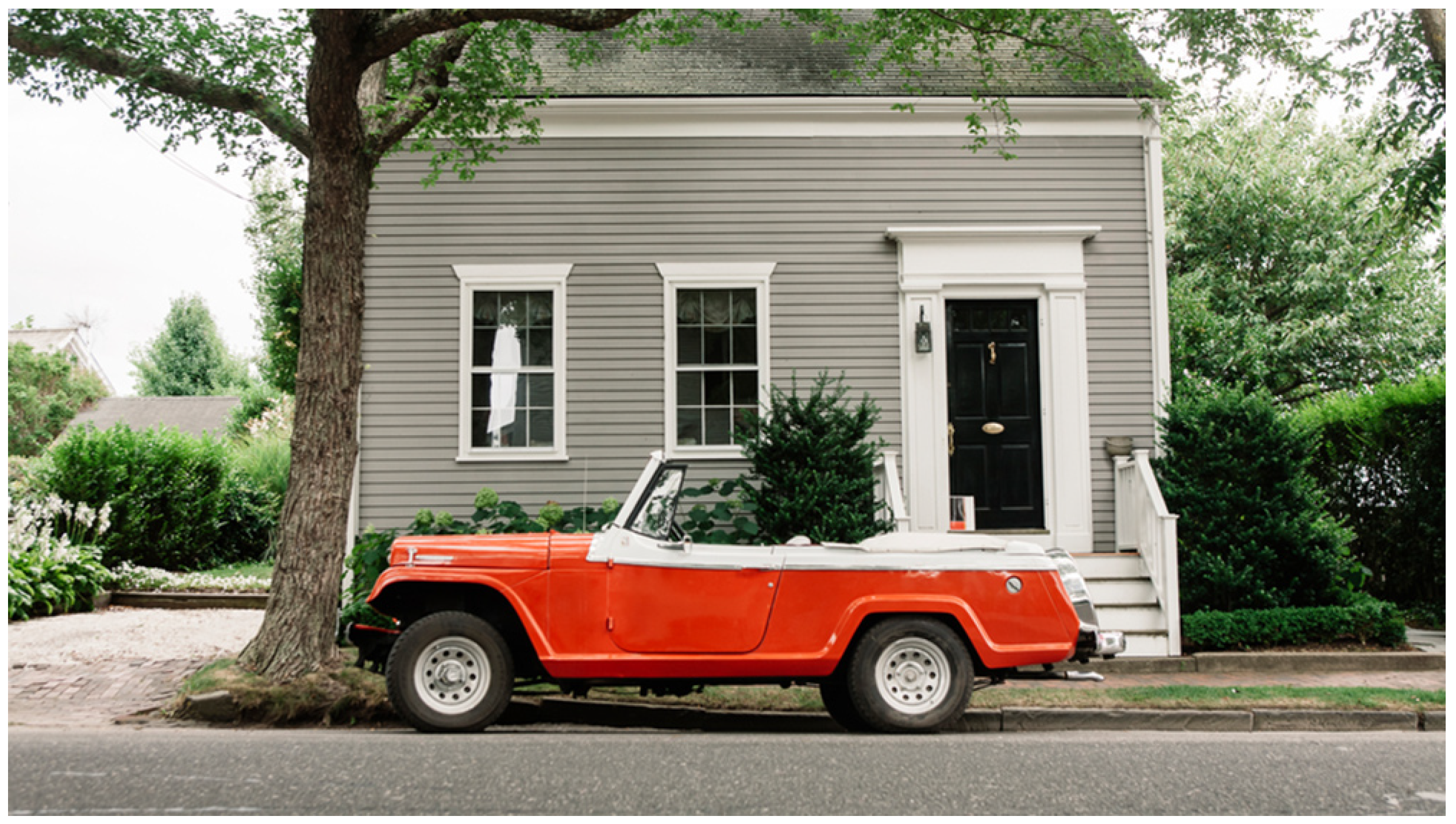
The features of a scene in an image are described using two-level descriptors. The first level includes features such as color and texture. The second level contains information regarding the objects present in the scene, such as a car and house, and the interaction of these objects. For example, the scene in Figure 1 can be described as “A red car in front of a grey house on a cloudy day”. Here, the low-level descriptors are red, grey, and cloudy, conveying information about the colors and textures present in the scene. The high-level feature descriptors are car, house, and in front of, characterizing the objects in the scene and how they interact.

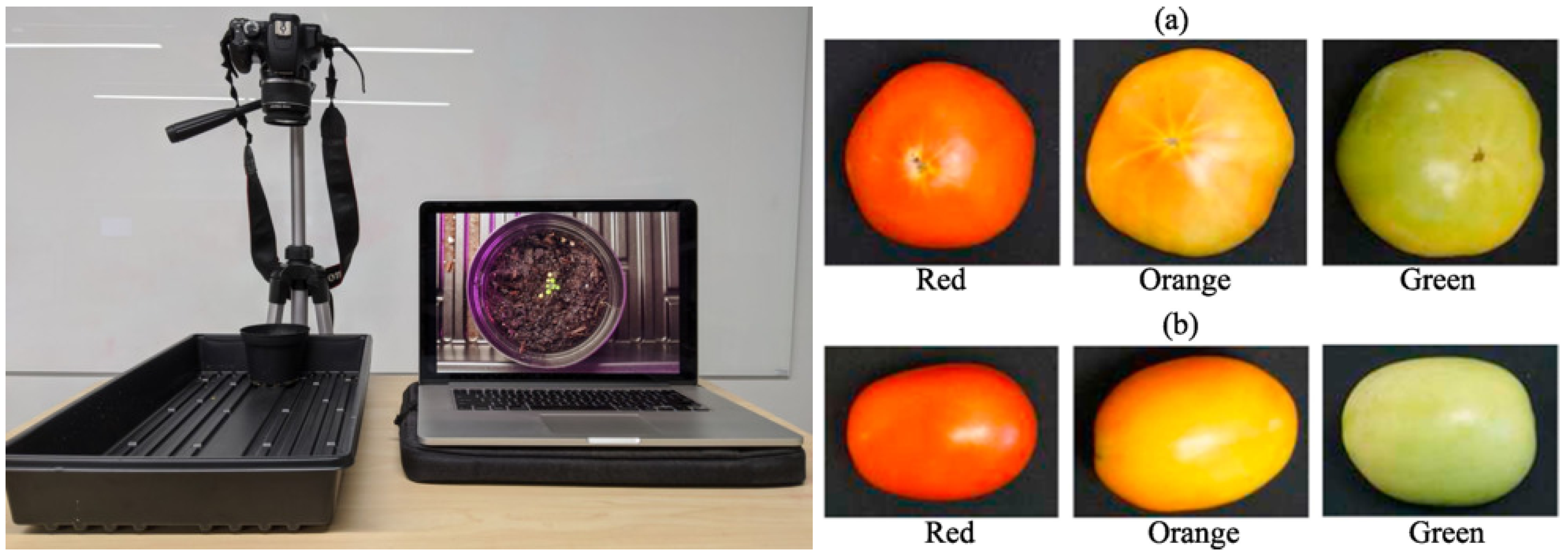
Similarly, various low-level and high-level descriptors explain the scene in the agricultural datasets. The descriptions in the literature commonly used shadow, sunlight, type of crop, background, color, occlusions, and other biological material terms to create a textual reference for the different types of scenes present in the images for a particular agricultural dataset. There are cases where the images are staged to create a real-world reference in the lab to decrease the data collection time (Figure 2) [94,95]. Here, the real-world descriptors are used to mimic the hue, saturation, lighting, etc., in the lab. The environment present in real-world image data is very complex. Various small and large features compose a scene. Creating an accurate description is very important. The following section discusses the various attempts at describing the scene found in agricultural image data and an effort to find common descriptors to establish a global definition for real-world agricultural datasets.

2.2. Scene Descriptors for Agricultural Imagery

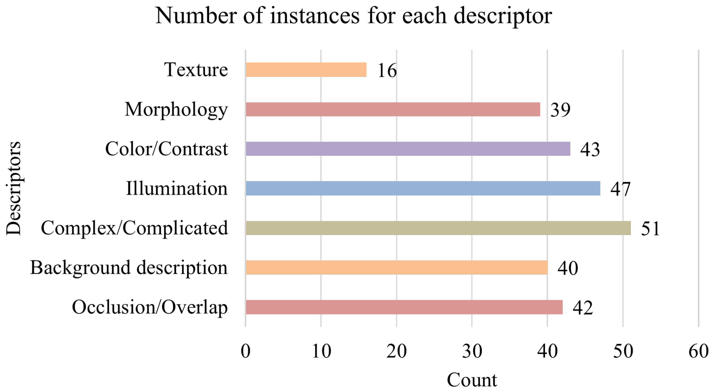
Analyzing all 63 articles from the literature, common descriptors were selected to characterize the scene in real-world agricultural applications and challenges with the scene for image processing. Semantically similar descriptors were kept in a single category, and the number of instances was counted when the authors used these descriptors to explain a scene. The low-level descriptors included color/contrast, texture, morphology, and illumination. The high-level descriptors were occlusion/overlap, background description, and complex/complicated. The count for the number of instances is provided in Figure 3. If an article described the minimal difference in color or the presence of low-contrast, a +1 count was added in the Color/Contrast descriptor. Similarly, if the similarity in texture between foreground and background was mentioned and varying lighting conditions were discussed, a +1 count was added to the Texture and Illumination descriptors, respectively. The Morphology descriptor was given a +1 count if the article discussed morphological features (shape, size, etc.). In the case of high-level descriptors, if the article expressed the interaction of foreground and background as complicated or complex to explain a scene, a +1 count was placed in the Complex/Complicated descriptor. When the article reported the types of objects or noise in the scene’s background, a +1 count was given to the Background description category. Finally, if the objects in the foreground or background were partially or fully blocking the object of interest in the particular study, +1 count was added to the Occlusion/Overlap descriptor. The Texture descriptor was used 16 times, the Morphology descriptor was used 39 times, the Color/Contrast descriptor was employed 43 times, the Illumination descriptor 47 times, the Complex/Complicated descriptor 51 times, the Background descriptor 40 times, and the Occlusion/Overlap descriptor was used 42 times.

Except for the Texture descriptor, the count of other descriptors used to explain a scene present in real-world agricultural image datasets was substantially higher. There is evidence of common patterns in the terminologies that can be used to derive a more universal definition for real-world agricultural datasets.

3. Low-Contrast Complex Background as a Unified Term

Since 2018, there has been a steady increase in the number of studies conducted each year for real-world deep learning agricultural applications. Each study attempted to define the scene in the images for each agricultural dataset. Common phrases and descriptions were observed but were limited to a focused scene. There is a need for a universal definition and unified terms to describe the scenes in real-world agricultural datasets. Defining a universal definition will assist the scientific community in performing more focused studies for agricultural scenes and develop deep learning models that can easily be generalized to other agricultural applications specific to low-contrast complex background situations. The increase in the number of publications each year and common themes within these publications indicates the growing importance of developing deep learning methods for real-world agricultural applications. Deep learning methods for real-world low-contrast complex background agricultural applications should be a sub-discipline within computer vision and machine learning applications in agriculture. A unified definition will be useful to further solidify this research space.

The Merriam–Webster dictionary defines complex (adjective) as “hard to separate, analyze, or solve” and contrast (noun) as “the difference or degree of difference between things having similar or comparable nature”. Based on the common descriptors used, the English language, and the literature reviewed, the low-contrast complex background can be used as a unified term and can be defined as follows:

“An image taken for an agricultural application can be said to contain low-contrast complex background if the object of interest has pixel value, saturation, and hue comparable to the entities present in the background, and/or the object of interest is either surrounded or occluded by other objects of interest, debris, biological materials, shadows, soil, and man-made materials of similar shape and sizes”.

4. Materials and Methods

4.1. Object Detection Models

The process of detecting an object using deep learning models involves two steps. The first step is to locate the objects of interest in the image and the second step is to classify those objects into different classes [96]. Deep convolutional neural networks are known for their feature extraction capabilities from images; hence, the current standard object detection architectures are based upon deep convolutional neural networks [97,98]. The object detection architectures are divided into two categories. The first one is two-stage object detectors. In two-stage architectures the task of object localization and object classification is divided into two different networks within the architecture. The main advantage of two-stage detectors is high accuracy of detection and the major drawback is slow detection speed. Some of the two-stage object detectors are as follows: RCNN [99], SPPNet [100], Fast RCNN [101], Faster RCNN [102], Mask RCNN [103], etc. The other type of architecture is one-stage object detectors. One-stage detectors do not separate the tasks of object localization and classification but directly perform both of the tasks through a single network. The main advantage of one-stage or single-stage detectors is the high speed of detection and the main limitation of these architectures is that the accuracy is comparatively lower than for the two-stage detectors. Some of the common one-stage detectors are the YOLO series [29,104,105,106], SSD [107], RetinaNet [108], etc.

4.1.1. Two-Stage Detectors

RCNN [99] used a deep convolutional neural network (DCNN) to extract image features and SVM to classify regions. In the case of SPPNet [100], it again used DCNN to extract image features and maps regions to propose the feature maps. Furthermore, spatial pyramid pooling is used to input multi-scale images to the DCNN. Fast-RCNN [101] uses DCNN to extract image features and maps down-scaled region proposals using a Region-Of-Interest (ROI) pooling layer to the feature maps. Faster-RCNN [102] uses a Region Proposal Network (RPN) to replace the DCNN and then the RPN shares feature maps with the backbone network. 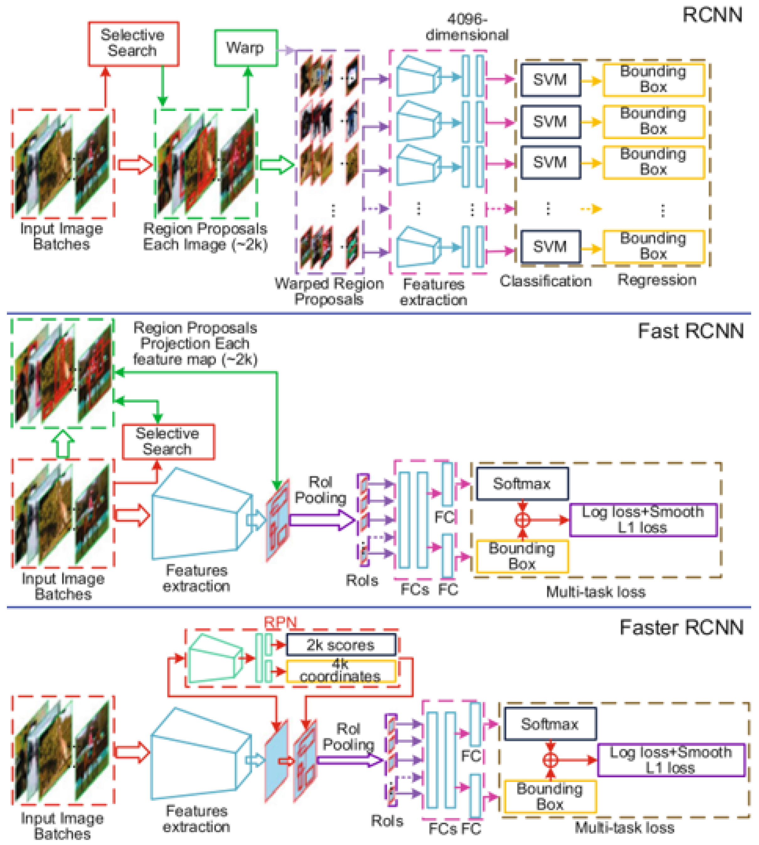Mask-RCNN [103] uses an ROI Align pooling layer instead of an ROI pooling layer improving the detection accuracy, and later combines training object detection and segmentation to improve accuracy in detection. The model architecture of the selected networks is shown in Figure 4.

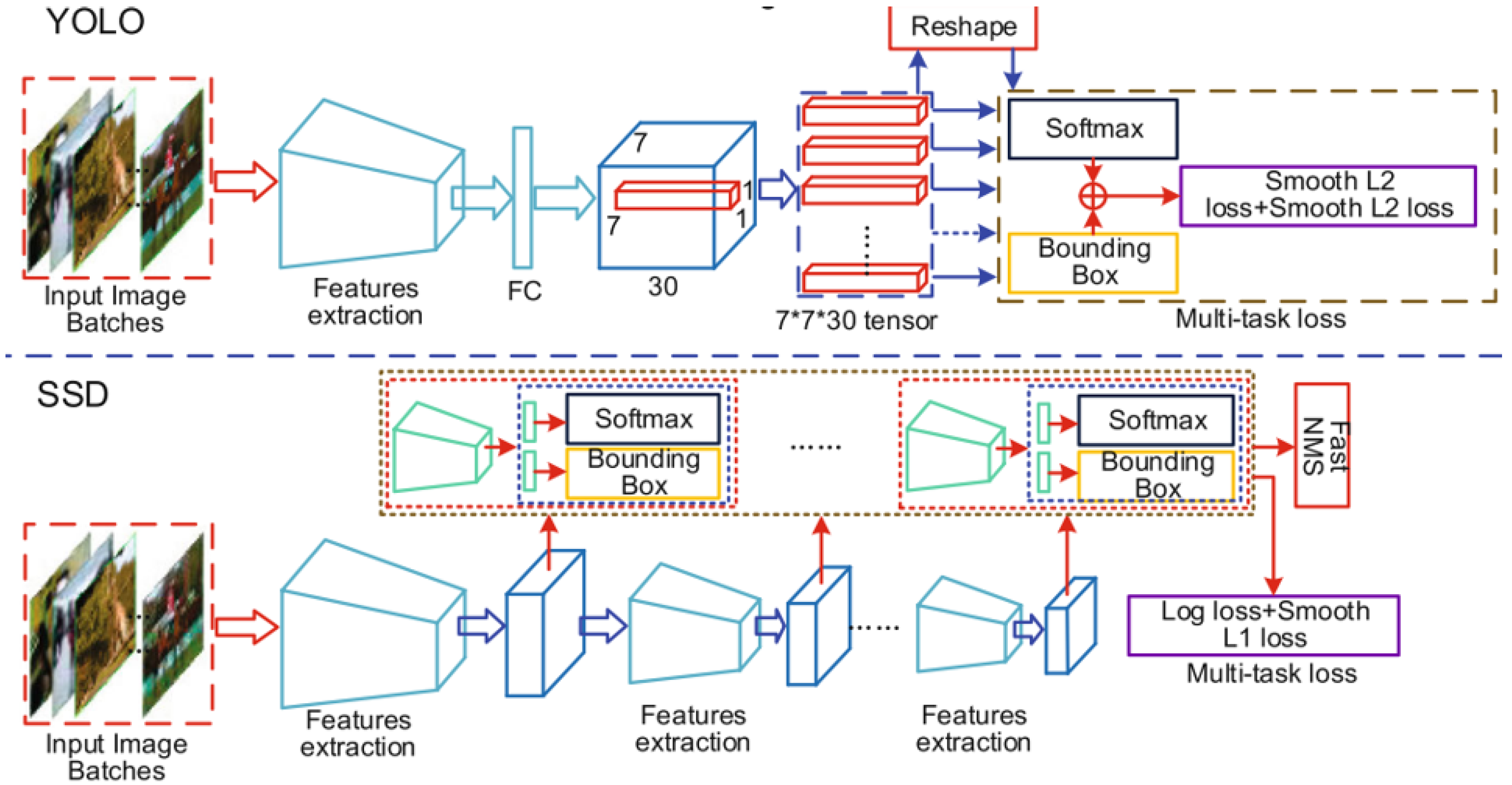
4.1.2. One-Stage Detectors

YOLOv1 [104] is an end-to-end single neural network and can implement class probabilities and bounding-boxes regression directly from a full image. YOLOv2 [105] introduced a new backbone network (DarkNet19) and used the k-means clustering algorithm to generate anchor boxes. YOLOv3 [106] used multi-level feature fusion to improve the accuracy of multi-scale detections and introduced a new backbone network (DarkNet53). YOLOv4 [29] experimented with different combinations of model features, such as Weighted-Residual-Connections (WRCs), Cross Mini-Batch Normalization (CMBN), Self-adversarial Training, etc. to achieve state-of-the-art results. It also introduced mosaic data augmentation as a new method for image augmentation. 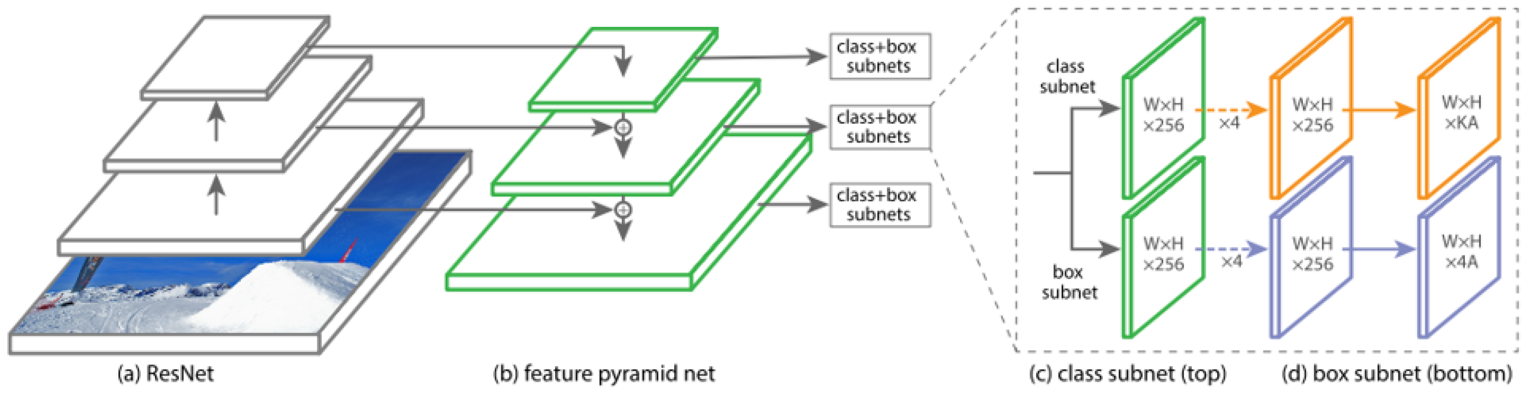SSD [107] presented a multi-layer detection mechanism and multi-scale anchor mechanisms at different neural layers. RetinaNet [108] used a feature pyramid network to extract features and developed a new focal loss for the model training. The model architecture of some of the networks is shown in Figure 5 and Figure 6.

4.1.3. Backbone Networks

Backbone networks for object detection are networks which are used for feature extraction in state-of-the-art models. The main objective of backbone networks is to identify important features in images and learn their characteristics, such as color, shape, texture, etc. With more and more complex applications, there is a need to improve the model performance. To achieve this, the network architecture becomes more and more complex. In some other situations where limited memory and computing power is available, lightweight networks are proposed, which simplify the architecture without affecting the feature extraction capacity. Some of the backbone networks are discussed below.

VGGNet [109] added more layers to AlexNet [97], increasing the network size to 16–19 layers. This improved the feature extraction capabilities of the network. VGG16 and VGG19 are widely known model architectures. ResNet or Residual Network [110] addressed the problem of gradient dispersion and gradient explosion problems which arises due to increasing the network by adding more layers. The authors achieved this by adding a residual to the output of the previous layer or stack of layers before creating the input of the next layer. ResNet50 to ResNet 152 are widely used as backbone networks. DetNet [111] was proposed as a backbone for object detection to address some shortcomings of generic backbone networks. DetNet used a dilated convolutional network instead of down-sampling some of the last layers to ensure enhanced resolution and a receptive field, which helps in locating large and small objects.

The backbones discussed above are complex in nature to deepen the depth of the network. However, some methods were also developed which sought to reduce the number of parameters in the network. This was performed to address the problem of storage space and processing time to develop a network that can be deployed on a mobile device. InceptionV1/V2/V3 [112,113,114] used kernel decomposition to make a lightweight model. Xception improved over InceptionV3 with a depth-wise separable convolution [115]. MobileNet [116] improved on the structure of the depth-wise separable method. MobileNetV2 [117] used short-cut connections like ResNet [110] along with depth-wise separable convolutions to improve performance.

In this study, Faster-RCNN and RetinaNet were used for comparing networks as they were available in TensorFlow API pre-trained on Imagenet and both networks were able to use ResNet50, ResNet101, and ResNet152 as backbone networks.

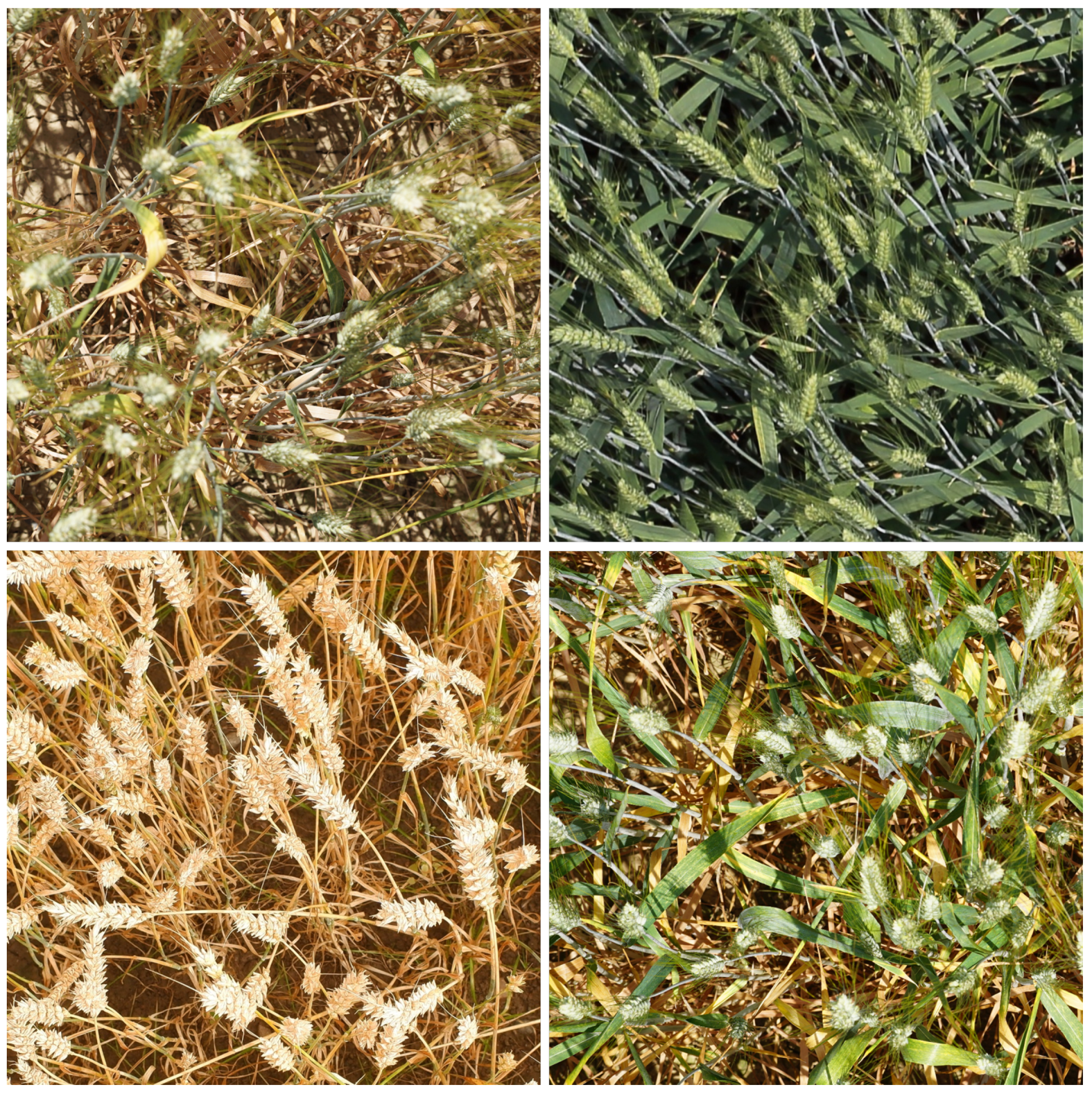
4.2. Global Wheat Dataset

The Global Wheat Dataset was used for this study as a reference dataset [118]. The Global Wheat Dataset is composed of more than 6000 images of 1024 × 1024 pixels containing 300k+ unique wheat heads with corresponding bounding boxes. The dataset includes images from 11 different countries and 44 unique measurement sessions. The dataset is a collection of images taken between 2016 to 2019 by nine different institutes and contains genotypes from North America, Asia, Europe, and Australia. The row spacing varied from 12.5 cm to 30.5 cm. The dataset covers varying sowing density (186 to 450 seeds/m²), soil types (loamy soil, silt-clay, etc.), and stage of growth (flowering to ripening). Cameras with different fields of view (7.1° to 45.5°) and focal length (7.7 mm to 60 mm) were employed to collect the imagery with the ground sampling distance varying from 0.2 mm/pixel to 0.56 mm/pixel. The dataset was chosen as it contains images with different lighting conditions and a range of hues with a complex background including occlusion of wheat heads. Selected example images from the Global Wheat Dataset are shown in Figure 7.

4.3. System and Training Specifications

In this study, the experiments were conducted using the deep learning framework provided by TensorFlow API (version: 2.8.0) from Google. Python 3.8.9 version was used for developing the object detection model experimental setup. For training the different neural networks, a machine running the Windows 10 professional operating system was used. The models were trained on Intel i-7 11700K 3.6 GHz CPU, 128 GB ram, and NVIDIA RTX 3090 28 GB VRAM GPU.

The Global Wheat Dataset was divided into three parts: 3000+ images in the training set, 1400+ in the validation set, and 1700+ in the testing set. Each model was trained for 80,000 steps.

4.4. Image Augmentations

Image augmentations are used in deep learning models to address the issue of overfitting during training. Furthermore, image augmentations help when large datasets cannot be collected and labeled for training a deep learning model. Also, image augmentations are used to resolve the problems associated with class imbalance [119]. Image augmentations either warp the data or carry out oversampling to artificially inflate the training dataset. Augmentations dealing with oversampling create synthetic instances and add them to the training set, whereas data warping augmentations transform existing images while preserving their labels [120]. Data warping image augmentations can be further classified as photo-metric augmentations and geometric augmentations. Photo-metric augmentations alter the pixel values of the features in the image, including brightness, contrast, hue, etc., whereas geometric augmentations change the layout of the image, such as by cropping, flipping, rotating, etc.

Some of the image augmentation methods are as follows:

Flipping: In this augmentation, the images are flipped by either the horizontal or vertical axis. It is one of the easiest to implement.

Color Space: An image consists of a 3D matrix, height, width, and color channels. Each element in this matrix consists of a pixel value for all three color channels. These pixel values or channels can be manipulated in order to perform image augmentations. One method is isolation of a single color channel. Changing the brightness, contrast, or saturation randomly is another way to alter the color space.

Cropping: Randomly cropping images can be used as a method of image augmentation. A mixed height and width patch can be cropped from anywhere in the image.

Rotation: In this augmentation, the image is rotated either to the left or right between 1° and 359°. This augmentation helps in training the model to make the objects appear in different orientations.

Noise Injection: Noise injection involves injecting a matrix of random values drawn from a Gaussian distribution within the image. Adding noise to images can help neural networks learn more robust features.

Color Space Transformations: One way to perform color space augmentation is to loop through the images and decrease or increase the pixel values by a constant value. Another quick color space manipulation is to splice out individual RGB color matrices. A further transformation consists of restricting pixel values to a certain min or max value. Also, individual color channels can be distorted to create various color gradient images.

Kernel Filters: Sharpening and blurring images are very widely known kernel filter augmentations. These filters work by sliding an n × n matrix across an image with either a Gaussian blur filter, which will result in a blurrier image, or a high-contrast vertical or horizontal edge filter, which will result in a sharper image along the edges.

Mixing Images: Mixing images together by averaging their pixel values is another approach to data augmentation.

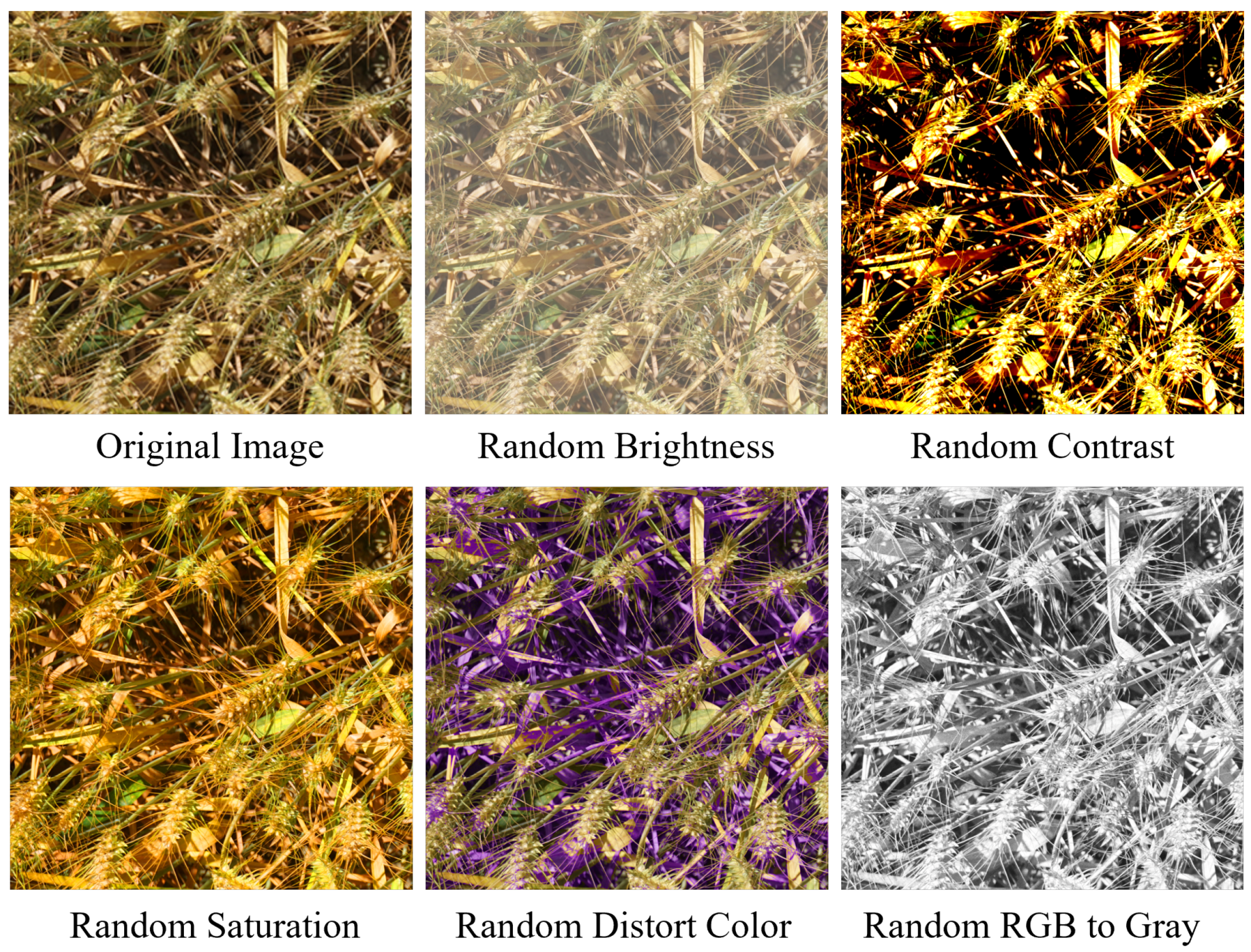
Random Erasing: Random erasing augmentation works by randomly selecting an n × m patch of an image and masking it with either minimum, maximum, mean pixel values, or random values. This technique was specifically designed to combat image recognition challenges due to occlusion. The authors of [119] demonstrated that not all the augmentations which were used in the study, including both geometric and photo-metric augmentations, were contributing equally towards improving a convolutional neural network’s model performance. Ref. [29] also reported similar results, mostly focused on using geometric augmentation to improve model efficacy. Therefore, in this study, five photo-metric augmentations which transformed the color space were tested to quantify their effects on object detection model performance in low-contrast complex background applications. The augmentations were random brightness, random contrast, random saturation, random distort color, and random Red-Green-Blue (RGB) to gray-scale conversion. Random brightness was applied by randomly selecting a brightness value from a uniform distribution; random contrast was applied on an image by randomly selecting contrast values from a uniform distribution; random saturation was applied on an image by randomly selecting saturation values from a uniform distribution; random distort color was applied by randomly selecting a color channel and randomly changing the pixel values; and random RGB to gray-scale was applied by randomly selecting an image and converting it into a gray-scale image. Visual examples of these augmentations on the Global Wheat Dataset are shown in Figure 8.

4.5. Performance Metrics

In supervised machine learning, it is necessary to provide ground truth labels to the model, which assists the model to learn important features in the data. For object detection, the ground truth is defined as a bounding box that gives the location of the object of interest in the image. The model is provided as rectangular coordinates with respect to the image Cartesian plane, i.e., x-coordinate for the upper left corner of the bounding box, y-coordinate for the upper left corner of the bounding box, with the width of the bounding box in pixels, and the height of the bounding box in pixels. To evaluate the performance of the object detection models, the overlap of the detected bounding box provided by the model and the ground truth bounding box is calculated.

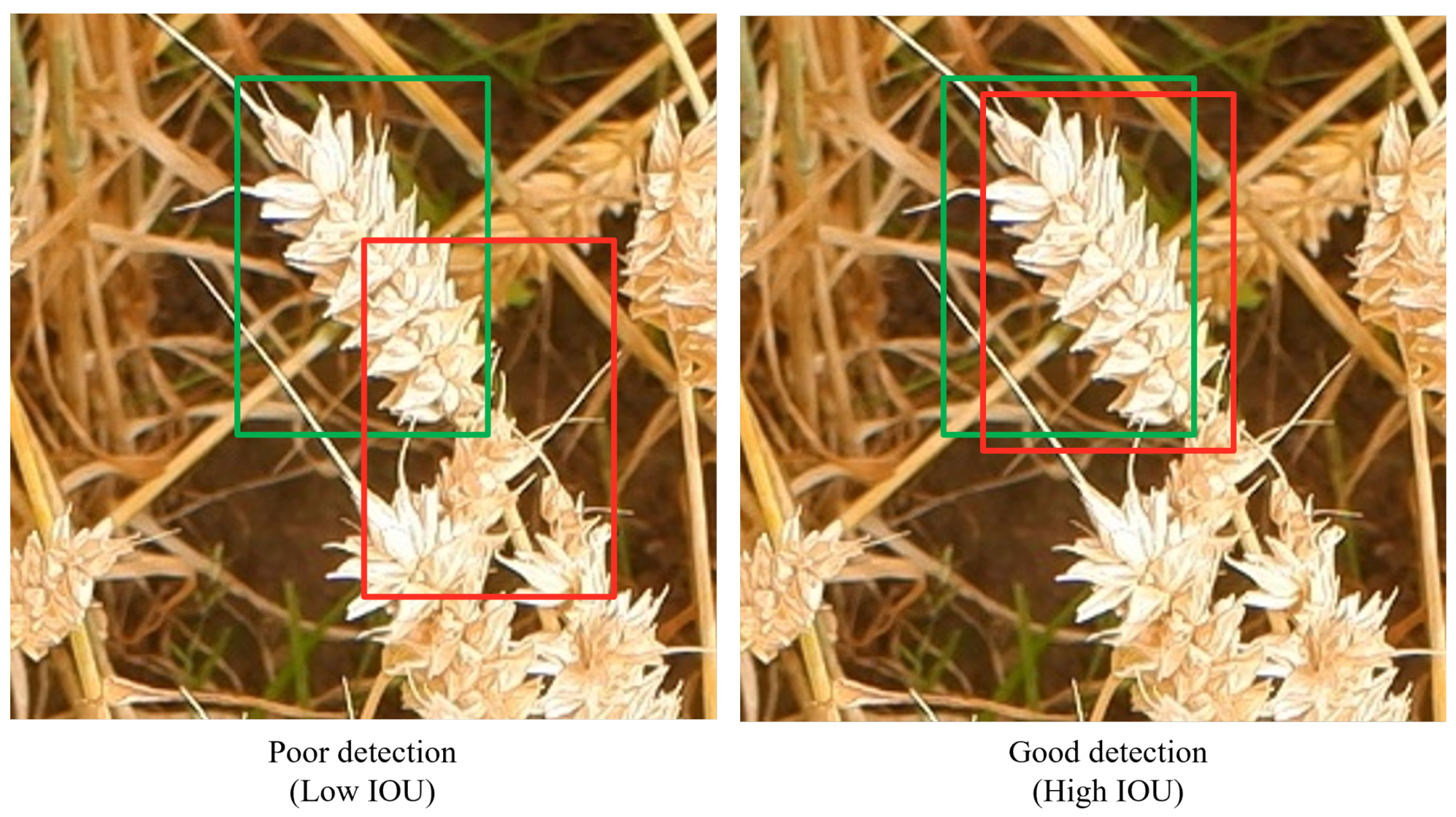
The Intersection-Over-Union (IOU) is the metric used to calculate the overlap of the predicted and ground truth bounding boxes (1). The IOU, also known as the Jaccard Index, is the ratio of the area of intersection of the two regions (boxes) in the numerator and the area of union of the two regions (boxes) in the denominator (Figure 9). If there is no overlap, but the boxes have common edges, the ratio will have a value of 0 as there is no intersection area. If there is a slight overlap, the ratio will achieve a value close to zero as the area of intersection is very small but the area of union is very large. As the overlap between the boxes increases, the area of intersection will increase and the area of union will decrease; therefore, the value of the ratio will approach 1. At full overlap, both the intersection and the union area are equal and the value of the ratio is 1.

$$IoU={\displaystyle \frac{area of intersection}{area of union}}$$

(1)

For a detection to be successful, the minimum percentage of overlap should be defined. This definition varies from project to project. In most cases, an IoU threshold of 0.5 (50% overlap) is considered a successful detection. Other common thresholds are 0.75 and 0.95 (75% and 95% overlap). By increasing the IoU threshold, the detected bounding box becomes highly accurate but it increases the difficulty and training time needed to detect a successful bounding box [121].

An object detection model provides multiple predicted bounding boxes for a single image. It is important to quantify how many predicted boxes were correct and how many out of all the ground truth boxes were detected. With every detection event, there will be some boxes which were predicted correctly depending on the set threshold (True Positive), there will be boxes that were not predicted correctly (False Positive), and finally, there will be some ground truth boxes which were never predicted (False Negative). These terms can be efficiently quantified as Precision and Recall. Precision can be defined as the proportion of the predicted positives that were actually correct (2) and Recall can be defined as the proportion of the actual positives that were predicted correctly (3).

$$Precision={\displaystyle \frac{True Positives}{True Positives+False Positives}}$$

(2)

$$Recall={\displaystyle \frac{True Positives}{True Positives+False Negatives}}$$

(3)

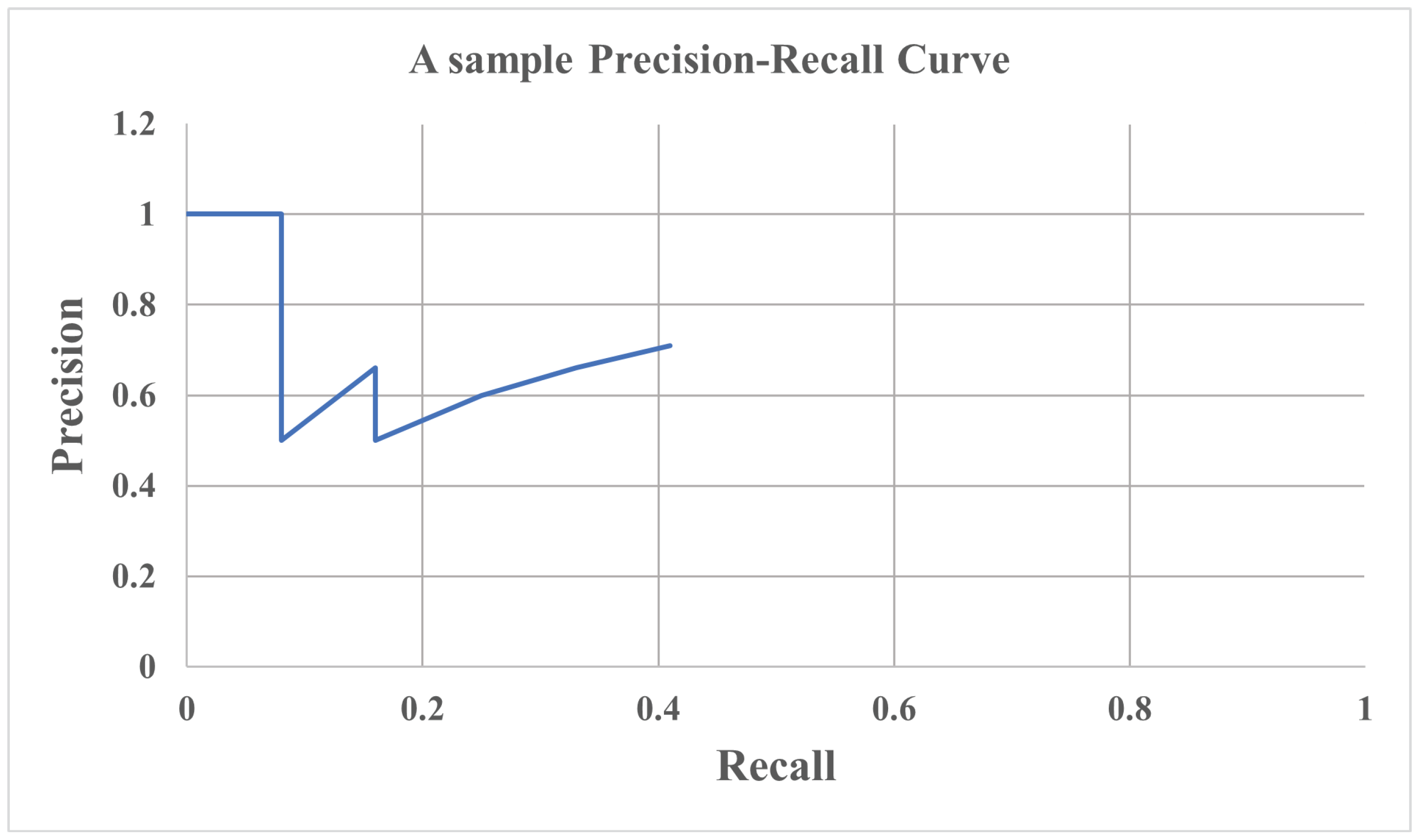
For all the classes present in a dataset, the precision and recall values can be calculated and can be plotted to create a Precision-Recall curve. The Precision-Recall curve is a good way to evaluate the performance of an object detection model. An object detection model is considered to be performing well if the precision of the model remains high as the recall of the model is increasing. A model sometimes can have high precision (0 False Positives) or high recall (0 False Negatives). Precision-Recall curves usually start with a precision value—the precision starts decreasing as the value of recall increases (Figure 10).

A drawback of Precision-Recall curves is that they cannot be compared from model to model. To address this, a quantitative value of Average Precision (AP) is used. The AP is the area under the curve of the Precision-Recall curve. AP is a numerical value which makes it easy to compare different models and can be defined as the average value of precision for all values of recall between 0 and 1 (4) [121]. Furthermore, if the APs of each class are averaged for all the classes, the resultant value is called the mean Average Precision (mAP).

$$AP={\displaystyle \frac{1}{n}}\sum _{r\in [0,0.1,....,1]}{\rho }_{interp\left(r\right)}$$

(4)

4.6. Experimental Design

In the first set of experiments, both of the selected object detection models, i.e., RetinaNet and Faster-RCNN, were trained on three different backbones. The backbones were as follows: ResNet50, ResNet101, and ResNet152. The models were compared on the COCO detection evaluation metrics, which include the average mAP at IOU = 0.5:0.05:0.95, the mAP at IOU = 0.50, the mAP at IOU = 0.75, the mAP for small objects: $area<{32}^2$ pixels, the mAP for medium objects: ${32}^2<area<{95}^2$ pixels, and the mAP for large objects: $area>{96}^2$ pixels.

In the second set of experiment, both RetinaNet and Faster-RCNN were trained using different color space augmentations for 80,000 steps. The backbone was fixed to ResNet101 for all the image augmentation experiments. The input image size was kept fixed at 1024 × 1024 pixels and no resizing was performed to avoid variations due to pixel interpolation. The color space augmentations used were random brightness, random contrast, random saturation, random distort color, and random Red-Green-Blue (RGB) to gray-scale conversion. Again, the models were compared on the COCO detection metrics.

Furthermore, all the models were compared on the total testing loss along with their overall mAP to quantify their effects on model fitting. Also, the percentage improvement of each model was compared either to a baseline or to the smallest model in the training. In this study, six different mean Average Precision (mAP) measures from the COCO evaluation metrics were used to quantify the performance of the different object detection models. The measures are, namely, the average mAP at IOU = 0.5:0.05:0.95, the mAP at IOU = 0.50, the mAP at IOU = 0.75, the mAP for small objects: $area<{32}^2$ pixels, the mAP for medium objects: ${32}^2<area<{95}^2$ pixels, and the mAP for large objects: $area>{96}^2$ pixels. The resolution of the images used for this study was 1024 × 1024 pixels, meaning small objects occupy less than 0.1% and large objects occupy more than 0.9% area. In just the training set of the Global Wheat Dataset containing 3658 images, out of 163,644 individual bounding boxes, there were 2109 small objects, 134,299 medium objects, and 27,236 large objects. There were 1477 images in the testing set, containing 44,331 bounding boxes, out of which 1132 were small objects, 24,851 were medium objects, and 18,348 were large objects. The mAP values were calculated at the end of each training session on the validation dataset.

5. Results

In

Table 2. Comparison of 1-stage and 2-stage detectors with different backbones.

Model	Backbone	Input	$\mathit{mAP}$	${\mathit{mAP}}_{50}$	${\mathit{mAP}}_{75}$	${\mathit{mAP}}_{\mathit{small}}$	${\mathit{mAP}}_{\mathit{medium}}$	${\mathit{mAP}}_{\mathit{large}}$
RetinaNet	ResNet50	1024 × 1024	0.381	0.782	0.320	0.022	0.308	0.489
RetinaNet	ResNet101	1024 × 1024	0.362	0.744	0.301	0.011	0.289	0.478
RetinaNet	ResNet152	1024 × 1024	0.366	0.746	0.313	0.009	0.288	0.488
Faster-RCNN	ResNet50	1024 × 1024	0.377	0.821	0.281	0.037	0.309	0.487
Faster-RCNN	ResNet101	1024 × 1024	0.403	0.838	0.325	0.050	0.336	0.503
Faster-RCNN	ResNet152	1024 × 1024	0.418	0.844	0.355	0.057	0.346	0.523

, the results from the first set of experiments are listed. In the case of RetinaNet, it was observed that the model with the smallest backbone, i.e., ResNet50, performed best compared to the other backbones for RetinaNet, with a mAP of 0.381. The other backbones had mAP values of 0.362 and 0.366 for ResNet101 and ResNet152, respectively. For the Faster-RCNN models, the model with the largest backbone performed best, i.e., ResNet152, with a mAP of 0.418. The backbones mAP values were 0.377 and 0.403 for ResNet50 and ResNet101, respectively.

Table 3. Comparison of different image augmentations for RetinaNet.

Augmentation	Backbone	Input	$\mathit{mAP}$	${\mathit{mAP}}_{50}$	${\mathit{mAP}}_{75}$	${\mathit{mAP}}_{\mathit{small}}$	${\mathit{mAP}}_{\mathit{medium}}$	${\mathit{mAP}}_{\mathit{large}}$
Baseline	ResNet101	1024 × 1024	0.362	0.744	0.301	0.011	0.289	0.478
Random Contrast	ResNet101	1024 × 1024	0.351	0.740	0.278	0.010	0.279	0.464
Random Brightness	ResNet101	1024 × 1024	0.385	0.781	0.328	0.019	0.311	0.494
Random Saturation	ResNet101	1024 × 1024	0.385	0.779	0.332	0.014	0.308	0.500
Distort Color	ResNet101	1024 × 1024	0.409	0.796	0.375	0.014	0.327	0.526
RGB to Gray	ResNet101	1024 × 1024	0.375	0.766	0.320	0.020	0.301	0.491

presents the results for the second set of experiments, i.e., the image augmentation methods for the RetinaNet model with a backbone of ResNet101. The baseline model with no data augmentations involved had a mAP of 0.362. The first augmentation performed was random contrast. The resultant mAP was 0.351, meaning the model performed poorly compared to the baseline. The next augmentation was random brightness, with a mAP of 0.385, representing a reasonable improvement compared to the baseline. The augmentation after random brightness was random saturation which was performed similarly, producing a mAP value of 0.385. The random distort color was the best performing augmentation compared to the other methods tested, giving a mAP of 0.409. Finally, the random RGB to gray-scale performed worse than the other methods except random contrast, with a mAP of 0.375.

The results for the second set of experiments with the Faster-RCNN model with a backbone of ResNet101 are shown in

Table 4. Comparison of different image augmentations for Faster-RCNN.

Augmentation	Backbone	Input	$\mathit{mAP}$	${\mathit{mAP}}_{50}$	${\mathit{mAP}}_{75}$	${\mathit{mAP}}_{\mathit{small}}$	${\mathit{mAP}}_{\mathit{medium}}$	${\mathit{mAP}}_{\mathit{large}}$
Baseline	ResNet101	1024 × 1024	0.403	0.838	0.325	0.050	0.336	0.503
Random Contrast	ResNet101	1024 × 1024	0.406	0.839	0.333	0.050	0.337	0.508
Random Brightness	ResNet101	1024 × 1024	0.414	0.847	0.344	0.055	0.343	0.515
Random Saturation	ResNet101	1024 × 1024	0.412	0.841	0.343	0.049	0.341	0.513
Distort Color	ResNet101	1024 × 1024	0.428	0.852	0.347	0.056	0.353	0.534
RGB to Gray	ResNet101	1024 × 1024	0.418	0.846	0.385	0.046	0.346	0.523

. The baseline mAP for Faster-RCNN with no augmentations performed was 0.403. It was comparably higher compared to RetinaNet’s baseline. This can be accounted for by Faster-RCNN being a two-stage detector, which is supposed to be more robust and accurate compared to RetinaNet, which is a singlestage detector. The first augmentation method tested was random contrast, providing a mAP of 0.406, which was a little greater than the baseline. A mAP of 0.414 was obtained when using the random brightness augmentation method during the training. This was a considerable increase compared to the baseline. The next augmentation was random saturation, giving a mAP of 0.412, which was slightly lower than the mAP for random brightness. The highest mAP, similar to the case with RetineNet, was provided by tthe random distort color augmentation method, with a value of 0.428. Lastly, the random RGB to gray-scale method gave a mAP of 0.418, which was comparable to the random brightness performance.

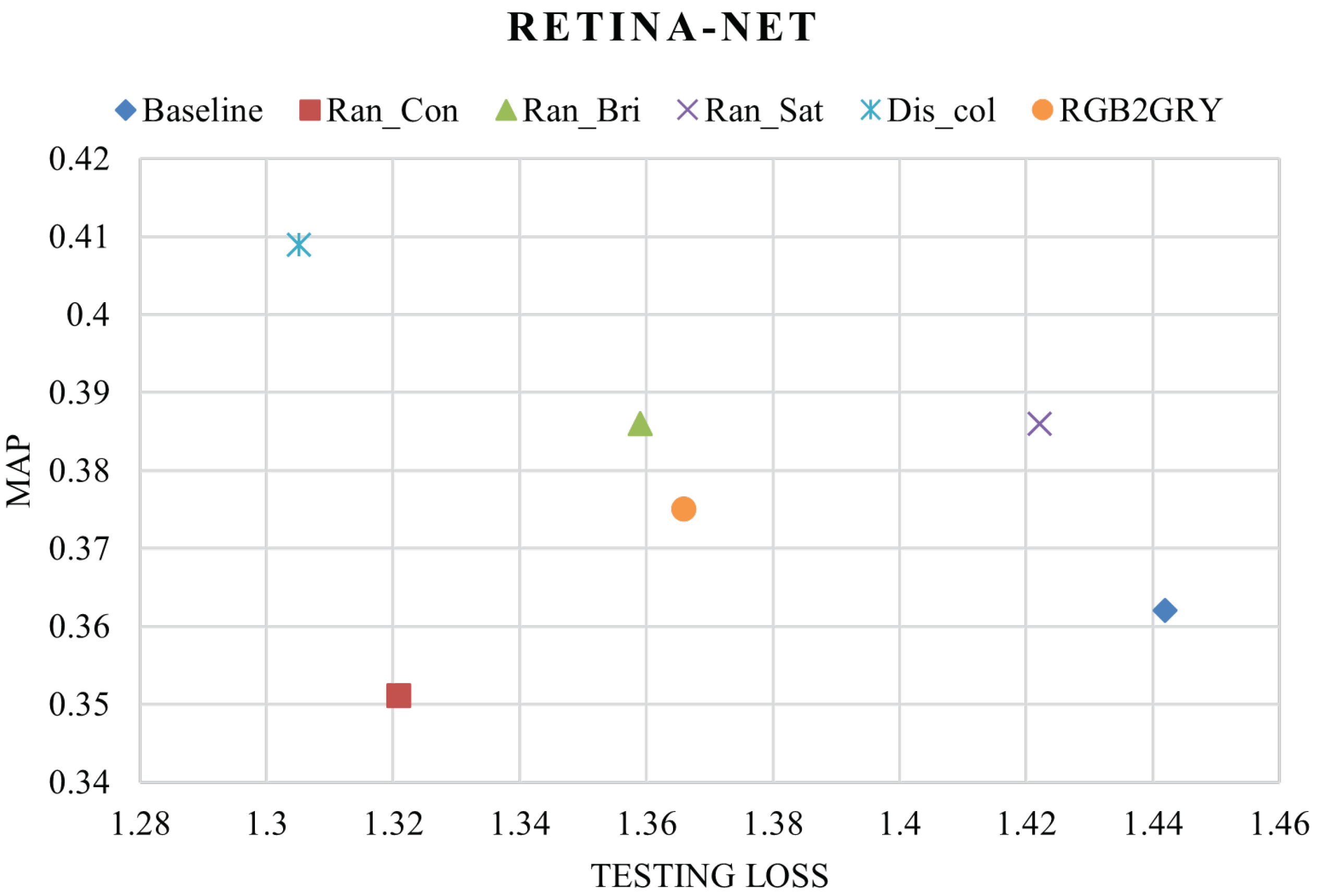
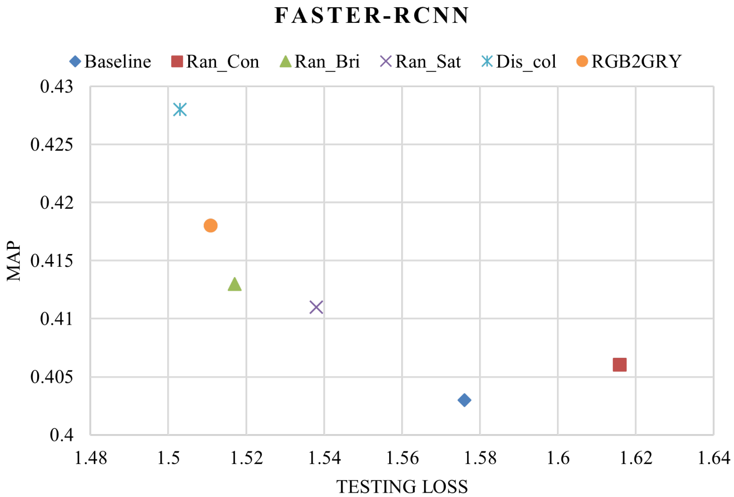
Furthermore, to better understand the performance for each image augmentation method, the testing loss was also compared along with the mAP for both the models. The methods which provided a higher mAP and a lower testing loss performed overall better compared to the other methods used to train the RetinaNet models. In Figure 11, random distort color is shown to have a testing loss of 1.305 with a mAP of 0.409, exhibiting the best performance for the RetinaNet model. Also, the lowest mAP value was produced by the random contrast trained model (0.362) and the maximum loss was produced by the baseline model (1.442). In the case of Faster-RCNN, a similar pattern was seen. The random distort color-trained model provided the least testing loss (1.503) and maximum mAP (0.428) when compared to the other Faster-RCNN-trained models in this experiment. For the Faster-RCNN models, the random contrast-trained model gave the highest training loss (1.616) and the baseline model had the lowest mAP (0.403) (Figure 12). In

Table 5. % Improvement using different image augmentations for RetinaNet.

Augmentation	$\mathit{mAP}$	% Improvement
Baseline	0.362	-
Random Contrast	0.351	−3.03%
Random Brightness	0.385	6.35%
Random Saturation	0.385	6.35%
Distort Color	0.409	12.98%
RGB to Gray	0.375	3.59%

, the % improvement provided by each augmentation method in the case of RetinaNet is displayed. The best performing augmentation method, i.e., random distort color, gave a model improvement of 12.98% and the random contrast method decreased the model performance by −3.03%. The percentage model performance improvements using different image augmentation methods for Faster-RCNN are presented in

Table 6. % Improvement using different image augmentations for Faster-RCNNt.

Augmentation	$\mathit{mAP}$	% Improvement
Baseline	0.403	-
Random Contrast	0.406	0.74%
Random Brightness	0.414	2.72%
Random Saturation	0.412	2.23%
Distort Color	0.428	6.20%
RGB to Gray	0.418	3.72%

. Similar to the RetinaNet case, the best performance improvement was obtained by using the random distort color method (6.2%). The least improvement with Faster-RCNN was produced by the random contrast method, i.e., 0.74%.

6. Discussion

In both the cases with RetinaNet and Faster-RCNN, it was observed that the image augmentation method random contrast either decreased the model performance or did not improve the model performance significantly compared to the baseline trained model. This can be attributed to the random contrast method while augmenting pixel values sometimes creating features which behave as negative examples during model training. These negative examples cause the model to learn them as features, which are not always indicative that the object of interest is present there. The next step will be to check how the random contrast augmentation method affects the model performance of the other augmentation methods.

All the other four types of image augmentation methods, which are random brightness, random saturation, random distort color, and random RGB to gray-scale were used in combination with random contrast to train new models for both RetinaNet and Faster-RCNN. They were then compared to the models which were trained using only the first four aforementioned image augmentation methods. In

Table 7. % Change while using random contrast augmentation with other image augmentation methods for RetinaNet.

Augmentation	$\mathit{mAP}$	Augmentation Combinations	$\mathit{mAP}$	% Change
Random Brightness	0.385	Brightness-Contrast	0.389	1%
Random Saturation	0.385	Saturation-Contrast	0.376	−2%
Distort Color	0.409	Distort Color-Contrast	0.409	0%
RGB to Gray	0.375	RGB to Gray-Contrast	0.394	5%

and

Table 8. % Change while using random contrast augmentation with different image augmentation methods for Faster-RCNN.

Augmentation	$\mathit{mAP}$	Augmentation Combinations	$\mathit{mAP}$	% Change
Random Brightness	0.414	Brightness-Contrast	0.412	−0.5%
Random Saturation	0.412	Saturation-Contrast	0.413	0.2%
Distort Color	0.428	Distort Color-Contrast	0.426	−0.4%
RGB to Gray	0.418	RGB to Gray-Contrast	0.419	0.2%

, the percentage changes in the model performance using all the other augmentation methods, in combination with random contrast for training both RetinaNet and Faster-RCNN, are presented. In both cases, random contrast did not provide any significant improvement except when used with random RGB to gray-scale for training RetinaNet. This may be because in combination with RGB to gray-scale, random contrast adds more difficult examples for the model to train on, making the model quite robust to unknown sets of images. Overall, random contrast, specifically when used with RetinaNet and Faster-RCNN to train on the agricultural dataset, did not provide any significant advantage. It either reduced or slightly increased the model performance when compared to the other image augmentation methods, which altered the pixel values to produce diversity in the dataset. In this study, a mid-size dataset was used. These findings might not apply to very small datasets as a small amount of examples are present for training. For small-scale datasets, further investigation is required to understand the effects of the data augmentations.

7. Conclusions

Low-level and high-level descriptors can be used to explain a scene in an image. Low-level features relate to color, texture, etc., while high-level features deal with objects and the relative information of those objects. For any image-based dataset, a description of the scene in the images is required to explain the information the images provide. Realworld agricultural datasets can have various low-level and high-level features present in them. Due to this, instances were found in the literature where different descriptions were given to explain the same type of scene. Numerous studies were reviewed that attempted to define scenes in real-world agricultural datasets to address the variations found in dataset descriptions. Later, common themes and patterns were identified, and a definition was provided to explain scenes in real-world agricultural datasets as low-contrast complex backgrounds.

Furthermore, the effects of model size and photo-metric image augmentation methods on one-stage (RetinaNet) and two-stage (Faster-RCNN) object detection deep learning models was studied. There are countless examples in the literature where it is stated that larger models perform better. There was a need to study the effects of model size while training on low-contrast complex background agricultural datasets. It was observed that for one-stage detectors, smaller models performed better compared to larger models. The model sizes were varied using different backbones for the networks, including ResNet50, ResNet101, and ResNet152. In the case of two-stage detectors, the backbone size did not affect the model performance, while with the bigger model, the model performance improved. In the second set of experiments, different photo-metric-based image augmentation methods were compared to understand the affect they have on model performance. It is often suggested that in the case of limited data availability, image augmentations can be used to make the deep learning model more robust and generalized. In the literature, it was found that some augmentations might affect the model performance negatively. Comparing different augmentation methods helped in understanding their effects on one-stage and two-stage detectors when training on low-contrast complex background applications. It was observed that except for the random contrast image augmentation method, every other method significantly improved model performance. Even when random contrast was used with other augmentation methods, there was no significant improvement.

In future research, the study can be expanded further to include other single-stage and two-stage detectors, which may have backbones similar to the ones used in this study. For models with different backbone structures, a broader comparison can be made to evaluate the effects of different backbone model structures containing a similar number of parameters. In addition, other datasets related to agricultural operations should be explored to verify the patterns observed in this study. This study used row crop images as a dataset; future studies can use image datasets from other agricultural focus areas, such as horticulture, floriculture, specialty crops, etc. This will help expand knowledge of objection detection models for low-contrast complex background applications in agriculture.