
Article

Research on Wake Characteristics of Dynamic Yawing Offshore Wind Turbine by Proper Orthogonal Decomposition


1
Research Center of Fluid Machinery Engineering and Technology, Jiangsu University, Zhenjiang 212013, China
2
Shimge Pump Industry (Zhejiang) Co., Ltd., Wenling 317525, China
3
School of Mechanical, Medical and Process Engineering, Queensland University of Technology, Brisbane 4001, Australia
*
Author to whom correspondence should be addressed.
Oceans 2026, 7(2), 25; https://doi.org/10.3390/oceans7020025
Submission received: 3 November 2025 / Revised: 3 February 2026 / Accepted: 12 February 2026 / Published: 9 March 2026
(This article belongs to the Special Issue Offshore Renewable Energy and Related Environmental Science)

Abstract

The wake that forms behind a yawing wind turbine is a complex flow region that can affect the performance of downstream turbines in offshore wind farms. It contains various flow features, including velocity deficit, shear layers, and vortex structures, which evolve in both time and space. Understanding this behavior is important for the design and operation of large-scale offshore wind farms. In this work, large-eddy simulations combined with proper orthogonal decomposition are used to study the wake development behind the National Renewable Energy Laboratory five-megawatt offshore wind turbine under both aligned and yawed inflow conditions. The results indicate that yawing the rotor leads to a lateral shift in the wake and increased asymmetry, with a stronger shear layer forming on one side. This asymmetry promotes enhanced mixing between the wake and the surrounding flow, contributing to a faster downstream recovery of the velocity field. The proper orthogonal decomposition analysis shows that the most energetic modes are associated with large-scale wake deflection and meandering, while higher-order modes correspond to smaller and less stable flow structures within the shear layer. The temporal evolution of these modes illustrates how the wake responds to the yaw maneuver and gradually reaches a new quasi-steady state. Overall, the study provides insight into the influence of yaw on wind turbine wake dynamics and demonstrates the applicability of combining large-eddy simulation with proper orthogonal decomposition for wake analysis in offshore wind farm studies.

1. Introduction

Wind energy has emerged as a cornerstone of the global transition to clean power. As nations accelerate efforts to cut carbon emissions and reduce reliance on fossil fuels, installed wind capacity has grown at an extraordinary pace, surpassing 1 terawatt worldwide in 2023 [1,2]. This expansion is driven by ambitious renewable energy targets and continuous advances in turbine technology, both onshore and offshore [3,4]. Yet despite these gains, aerodynamic challenges persist at the wind farm scale. Chief among them is the wake generated by operating turbines, a region of reduced velocity and elevated turbulence that directly impacts the performance and structural integrity of downstream machines [5,6].
Turbine wakes are characterized by a pronounced velocity deficit and enhanced turbulent mixing relative to the incoming flow [7,8]. As the wake propagates downstream, it expands and interacts with neighboring turbines, often leading to power losses of 10–25% in densely packed wind farms, depending on atmospheric conditions [9]. These interactions also amplify fatigue loading, increasing maintenance costs and shortening component lifespans.
To mitigate these effects, engineering wake models, such as the Jensen top-hat model and the Gaussian model proposed by Bastankhah and Porté-Agel, are widely used for wind farm layout optimization and control due to their computational efficiency [10]. However, their simplified assumptions limit their ability to capture the full complexity of real turbine wakes, including unsteady shear-layer instabilities, wake meandering, and coupling with the atmospheric boundary layer. For deeper physical insight, high-fidelity numerical simulations have therefore become indispensable.
Computational Fluid Dynamics (CFD) now plays a central role in wind energy research [11,12]. While Reynolds-Averaged Navier–Stokes (RANS) models provide fast and computationally efficient steady-state solutions [13,14], they inherently filter out transient flow dynamics. In contrast, Large-Eddy Simulation (LES) resolves the large-scale turbulent structures while modeling only the smallest scales [15]. This capability enables accurate representation of time-dependent phenomena such as yaw-induced wake asymmetry, atmospheric stability effects, and rotor-generated vortex dynamics [16,17]. Although computationally demanding, LES provides the spatial and temporal resolution required to inform next-generation wind farm control strategies.
Recent LES studies have further emphasized the importance of transient and atmospheric effects [18]. Notably, Xiao et al. [19] released a comprehensive LES dataset capturing wind farm dynamics over a full diurnal cycle, demonstrating how changing atmospheric stability conditions modulate wake recovery and power output. Such work highlights the value of high-fidelity simulations in bridging atmospheric physics and operational wind farm performance.
At the same time, increasing attention has been directed toward the distinction between fixed-bottom and floating offshore wind turbines. Floating platforms introduce additional degrees of freedom, including surge, pitch, and heave, which couple with aerodynamic forces and alter wake development. For instance, Alkhabbaz et al. [20] demonstrated that surge motion in an NREL 5 MW floating turbine increases wake meandering and reduces power output by up to 8% compared to fixed-bottom configurations. Similarly, Xie et al. [21] showed that platform-induced inflow variations delay wake recovery and elevate fatigue loading. Although the present study focuses on a fixed-bottom turbine to isolate the purely aerodynamic response to active yaw control, these findings underscore the need for tailored wake-steering strategies in floating offshore wind farms.
Even with LES, the resulting flow fields are high-dimensional and complex. To extract meaningful physical insights, we employ Proper Orthogonal Decomposition (POD), a powerful modal analysis technique that decomposes turbulent flows into orthogonal spatial modes ranked by their energy content [22]. Unlike conventional spectral methods, POD yields data-driven modes that represent the dominant coherent structures of a given flow, including wake deflection, shear-layer instabilities, vortex shedding, and turbulence cascades [23,24]. Each spatial mode is associated with a temporal coefficient, enabling independent tracking of the evolution of different flow scales. This framework has proven valuable for constructing reduced-order models of wake dynamics and for linking coherent flow structures to control inputs [25,26].
Building on these modal decomposition techniques, recent studies by our group have advanced wake characterization through hybrid data-driven and physics-informed approaches. Luo et al. [27] developed a physics-consistent framework for reconstructing unsteady turbine wakes from sparse sensing, enabling control-oriented reduced-order modeling. This was further extended using physics-informed machine learning to reconstruct yawed wake fields from limited measurements [28]. Complementary work has demonstrated dynamic wake reconstruction using virtual LiDAR data [29], Physics-Informed Neural Networks [30], and reduced-order modeling combined with sparse observations [31,32]. These efforts underscore the growing synergy between modal analysis, sparse sensing, and machine learning for real-time wake estimation and control.
However, most previous POD-based investigations focus on statistically steady turbine wakes. The transient phase associated with active yaw maneuvers, during which wake asymmetry, enhanced turbulent mixing, and unsteady forcing coexist, remains poorly understood. Key questions remain unanswered: how is energy redistributed among POD modes during yaw transients, and how long does the wake require to re-stabilize once yawing ceases? Addressing these questions is essential for the development of effective dynamic wake-steering strategies.
The present study addresses this gap. Using LES coupled with time-resolved POD analysis, we investigate the unsteady wake dynamics of an NREL 5 MW offshore wind turbine under both aligned and dynamically yawed operating conditions. We quantify not only the magnitude of wake deflection, but also the redistribution of turbulent energy across spatial scales and the relaxation time following yaw maneuvers. By elucidating the dual role of yaw as both a geometric wake deflector and a turbulence amplifier, this work provides actionable insights for optimizing wake-steering strategies in real-world wind farms.
The remainder of this paper is organized as follows. Section 2 details the numerical methodology, including the large-eddy simulation (LES) framework, actuator line modeling of the NREL 5 MW turbine, the Smagorinsky–Lilly subgrid-scale closure, and the proper orthogonal decomposition (POD) formulation for extracting coherent wake structures. Section 3 presents a time-resolved analysis of dynamic wake evolution under yaw control, quantifying lateral deflection, velocity recovery, vorticity dynamics, and, through POD, the redistribution of turbulent energy across spatial scales during transient maneuvering. Section 4 synthesizes these findings to elucidate the dual role of yaw as both a geometric deflector and a turbulence amplifier, offering actionable insights for dynamic wake steering in offshore wind farms.

2. Methodology

2.1. Large Eddy Simulation

In this study, a Large Eddy Simulation (LES) is carried out to examine the dynamics of the wake that develops downstream of a wind turbine. LES relies on solving the filtered form of the Navier–Stokes equations, where only the large-scale turbulent motions are explicitly resolved, while the smaller scales below a prescribed cutoff length are filtered out and modeled [33]. The governing equations for the dimensionless velocity field, u , and the pressure, p , in incompressible flows can be expressed as:
u i t + u i u j x j = p x i + 1 R e 2 u i x j x j τ i j x j + f i   ,
u i x i = 0 ,
where i , j   {1, 2, 3} represent the streamwise ( x ), wall-normal ( y ), and spanwise ( z ) directions, respectively. The Reynolds number is defined as R e = U D / v , where U is the inlet velocity, D is the rotor diameter and v is the kinematic viscosity of the fluid, which have been used as reference variables (namely, x = X / D , y = Y / D , z = Z / D and u i   = U i U ).
The subgrid-scale (SGS) stress tensor τ i j = u i u j ¯   u i ¯ u j ¯ is decomposed into isotropic and anisotropic parts. The isotropic component 1 3 τ k k δ i j is absorbed into the modified filtered pressure p ¯ , while the anisotropic part is modeled using the Smagorinsky–Lilly model:
  τ i j 1 3 τ k k δ i j = 2 v t S ¯ i j
v t = ( C s ) 2 S ¯  
with eddy viscosity v t , Smagorinsky constant Cs = 0.13, grid filter width Δ = Δ x Δ y Δ z 1 3 , and resolved strain-rate tensor defined as:
  S ¯ i j = 1 2 u ¯ i x j + u ¯ j x i
This formulation is appropriate for high-Reynolds-number incompressible flow where viscous effects are confined to the near-wall region and the turbine is represented via actuator methods without resolved blade boundary layers.
The final element in Equation (1),   f i , represents the force per unit volume that simulates the aero dynamic forces imposed by the turbine blades on the fluid through the actuator line method, which will be elucidated in Section 2.2. The governing equations are resolved with a second-order accurate centered finite difference method on a staggered Cartesian grid and a hybrid low-storage third-order-accurate Runge–Kutta method for time integration [33].

2.2. Actuator Line Model

For the purpose of adequately simulating the unsteady aerodynamic loading of the rotor with computational efficiency, the Actuator Line Method (ALM) is applied in this work. By such a method, an optimum balance between the fully resolved blade simulation and the primitive actuator disk model is obtained such that the three-dimensional flow interaction between the wake and the turbine blades can be realistically simulated [34]. The computed aerodynamic forces by the ALM are then merged in the momentum equations of the Large Eddy Simulation (LES) in the form of body forces over an extended computational domain. The actuator line model sketch employed in this paper is illustrated in Figure 1, where it indicates the discretized blade elements, the airfoil aerodynamic forces, and the Gaussian projection of the body forces on to the computational mesh.
In this work, the rotor blades are represented using the actuator line method (ALM) introduced by Sørensen and Shen [35]. In this approach, each blade is treated as a rotating line that is divided into small segments along the span. For every segment, the aerodynamic forces are obtained from pre-tabulated airfoil data, which provide the lift ( C L ) and drag ( C D ) coefficients as functions of the local flow conditions. With the local chord length c , twist angle ϕ , and air density ρ known, the lift and drag forces per unit length are determined from the following relations:
F L = 1 2 ρ u r e l 2 C L ( α ) c F ,
F D = 1 2 ρ u r e l 2 C D ( α ) c F ,
where u r e l is the relative velocity seen by the blade section and α denotes the angle of attack. The factor F , is a modified Prandtl tip-loss correction [36], which accounts for the loss of efficiency near the blade tip and root caused by three-dimensional flow effects.
Once the aerodynamic forces are obtained, they are projected onto the flow as body forces applied normal to each actuator line. A Gaussian kernel is used to smooth these forces in space, reducing numerical oscillations and approximating the physical spreading of vorticity in the real flow.
The entire turbine, including the blades, nacelle, and tower, is modeled using the Actuator Line Model (ALM). The blades are represented as rotating lines composed of discrete aerodynamic force elements, whereas the nacelle and tower are treated as stationary actuator lines. For these components, drag forces are calculated based on their projected frontal area and the local flow conditions. The aerodynamic forces are obtained from airfoil look-up tables and distributed onto the flow field using a Gaussian smoothing kernel, following the standard SOWFA implementation [37]. This modeling strategy eliminates the need for body-fitted meshes around complex turbine geometries and is consistent with common large-eddy simulation practices in wind turbine research.

2.3. Simulation Setup

For this study, the NREL 5 MW reference wind turbine [37] is used as the base model. The nacelle, blades, and tower are all modeled using the above-described Actuator Line Method. Table 1 shows the main geometry and performance parameters of the turbine. The turbine is a three-bladed upwind turbine with a rotor size of 126 m, hub height of 90 m, and a rated speed of 9.15 rpm and tip-speed ratio of 7.5.
These operational parameters correspond to the rated (maximum power) condition of the NREL 5 MW reference offshore wind turbine under a wind speed of 11.4 m/s, as defined in the original design report by Jonkman et al. [37]. At this operating point, the turbine achieves peak aerodynamic efficiency with a power coefficient Cp ≈ 0.48, and the TSR of 7.5 is standard for modern three-bladed horizontal-axis wind turbines. This choice ensures consistency with widely used LES benchmark studies of the same turbine model [38].
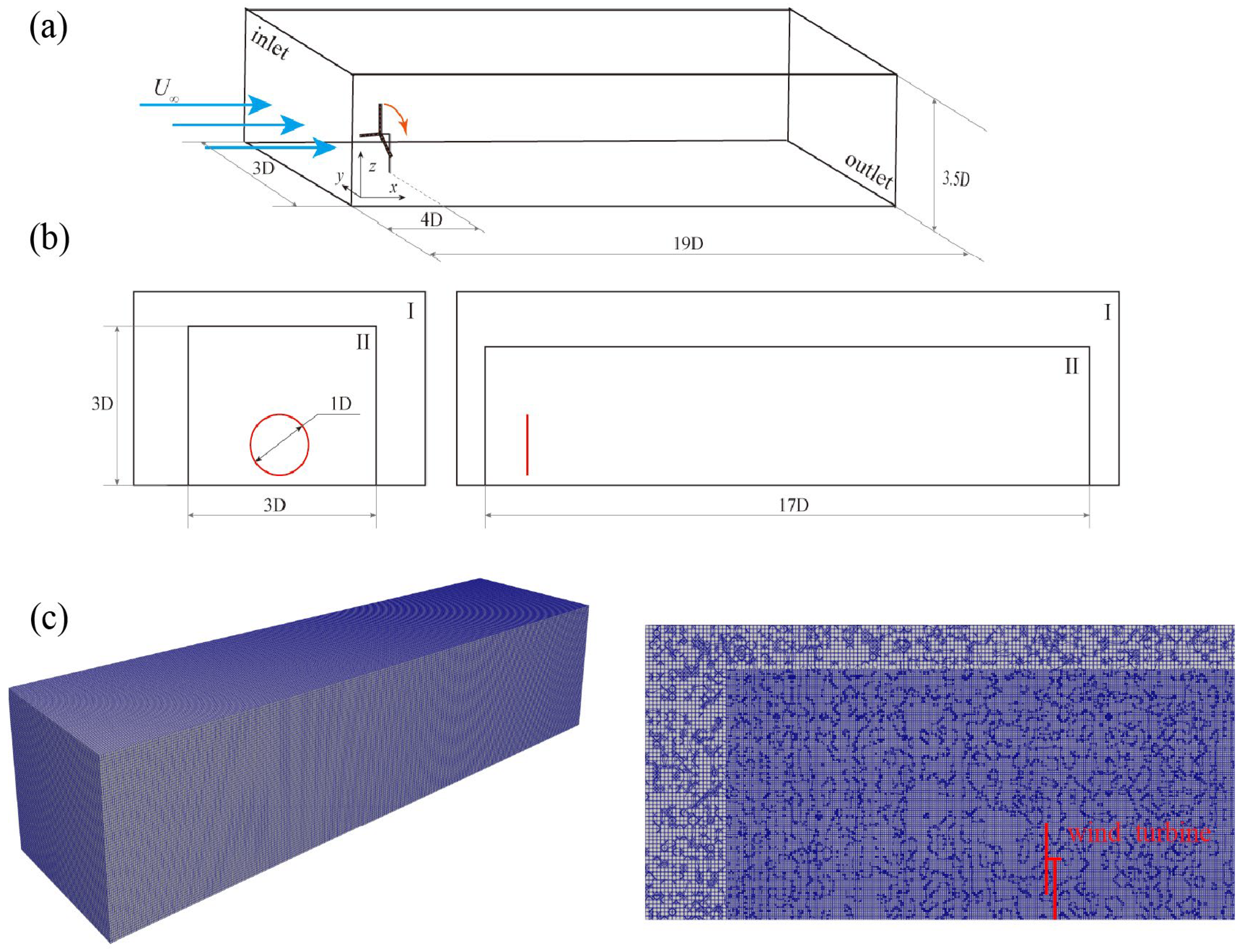
The layout of the computational domain used for the LES is shown in Figure 2a. The flow field extends 15 D downstream and 4 D upstream of the turbine, with both lateral and vertical dimensions set to 3.5 D to limit blockage effects. A uniform inflow velocity of U = 8 m/s with 6% turbulence intensity is prescribed at the inlet. At the outlet, a zero-gradient (Neumann) condition is applied for both velocity ( u n = 0 ) and pressure ( p n = 0 ). The top and lateral boundaries are modeled as slip walls ( u i n = 0 ), and the ground is a no-slip wall with roughness length z0 = 0.001 m, representative of typical offshore conditions with moderate wave activity [39,40].
A structured hexahedral mesh is utilized in the whole computational domain. In order to have a proper resolution of the wake dynamics, the local mesh refinement was performed by using the refine Mesh utility for the near-wake region (Region II of Figure 2b). The final grid used contains around 25 million cells that allows sufficient resolution of the rotor near-wake and the dominant large-scale structures. The time step is chosen such that the maximum Courant–Friedrichs–Lewy (CFL) number is always below 0.5 to ensure numerical stability and convergence of the transient LES solution. This CFL threshold is consistent with best practices for LES of wind turbine wakes [41], which recommend CFL ≤ 0.5 to accurately resolve wake vortex dynamics and avoid numerical dispersion.
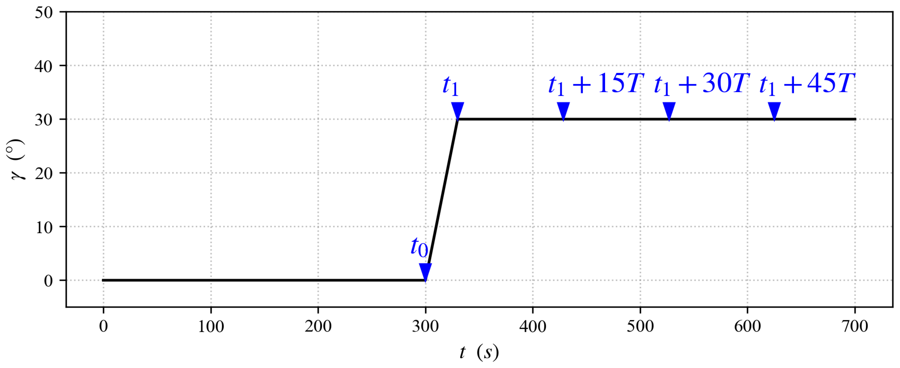
To capture how the wake develops and adjusts during a yaw maneuver, the total simulation time is set to 700 s. At the initial time t 0 , the wind turbine operates under an aligned inflow with zero yaw angle. At t 1 , the rotor begins to rotate about the vertical axis at a constant yaw rate until the yaw angle reaches γ = 30 . Once this target angle is achieved, the turbine remains at this orientation for the remainder of the simulation.
The evolution of the yaw angle with time is presented in Figure 3, where five key sampling instants are indicated. These correspond to different stages of the yaw maneuver and the subsequent wake adjustment:
t 0 : before yawing, aligned inflow condition,
t 1 : end of yaw motion,
t 1 + 15 T , t 1 + 30 T , and t 1 + 45 T : later instants corresponding to multiples of the rotor rotation period T .
These sampling points are selected to capture the transient development and stabilization of the yawed wake. In the following sections, the velocity and vorticity fields at these instants are analyzed to examine the wake’s dynamic response to yaw misalignment and the associated flow structures.

2.4. Model Validation and Computational Details

To ensure the reliability of the numerical framework, a series of validation and consistency checks were performed before the main yaw-maneuver simulations. The computational methodology employed here follows best practices for LES of wind-turbine wakes and is consistent with prior benchmark studies such as those by Porté-Agel et al. [15] and Sørensen and Shen [35].
(a)
Grid-independence and time-step sensitivity.
Three grids of increasing density (15 million, 25 million, and 37 million cells) were examined to assess spatial convergence. The mean axial velocity and turbulence intensity along the centerline were used as evaluation metrics. Differences between the two finest grids remained within 2%, confirming that the 25-million-cell mesh adopted in this work provides sufficient resolution for the large-scale wake structures. The physical time step t was selected so that the maximum Courant–Friedrichs–Lewy (CFL) number stayed below 0.5, ensuring both numerical stability and accurate temporal resolution of vortex dynamics. Additional tests with t reduced by 30% yielded less than 1% variation in time-averaged velocity statistics, confirming time-step independence.
(b)
Sub-grid-scale model and boundary conditions.
The standard Smagorinsky–Lilly formulation was adopted for the sub-grid stress tensor with a model constant Cs = 0.13. Near-wall regions employed the logarithmic wall law for rough surfaces, characterized by a surface roughness length z0 = 0.001 m to mimic offshore conditions [42].
(c)
Validation against reference data.
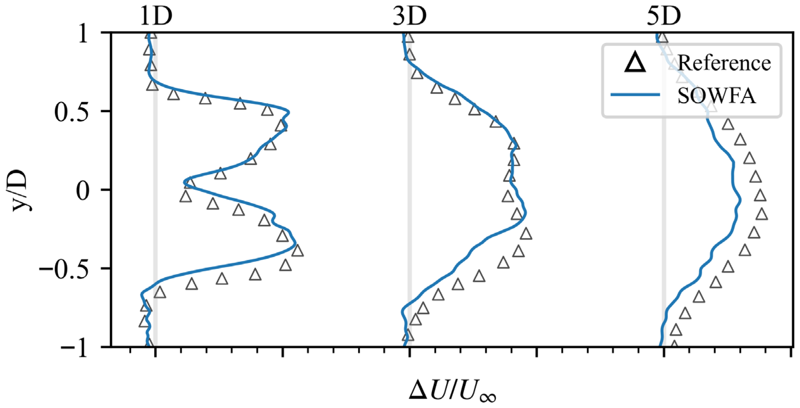
A preliminary aligned-inflow simulation of the NREL 5 MW turbine was compared with published LES data [41] as shown in Figure 4. The averaged velocity deficit at 1D, 3D and 5D downstream agreed within 5% of the reference, and the wake recovery rate was nearly identical. The radial profile of streamwise velocity matched previous numerical predictions both qualitatively and quantitatively, confirming the capability of the present model to reproduce the main flow physics of turbine wakes.
To quantify agreement, the mean absolute error (MAE) between our simulation and the reference LES data is <5% across all downstream locations. The Pearson cross-correlation coefficient is r = 0.985, confirming excellent linear correspondence. These metrics confirm that the present framework accurately captures both the shape and magnitude of the wake deficit evolution.
(d)
Computational resources and uncertainty assessment.
All simulations were carried out on the High-Performance Computing cluster of Jiangsu University. Each case utilized 512 cores distributed over 32 nodes, with a total wall-clock time of approximately 4.6 × 10⁵ CPU hours. Parallel scaling tests demonstrated near-linear performance up to 512 processors, validating the efficiency of the domain-decomposition strategy and the stability of the solver for long transient integrations. The estimated numerical uncertainty in the mean streamwise velocity at 5 D downstream was ±3.1%, while that of turbulence intensity was ±4.8%. These values are acceptable for high-fidelity LES and indicate that the conclusions drawn in subsequent sections are statistically robust.
Overall, these verification and validation exercises demonstrate that the present LES–ALM framework accurately captures the essential physics of turbine wakes under both aligned and yawed inflow conditions while maintaining computational tractability for long transient simulations.

2.5. Proper Orthogonal Decomposition (POD)

To extract dominant coherent structures from the high-dimensional LES velocity field, Proper Orthogonal Decomposition (POD) is employed. POD provides an optimal low-dimensional representation of turbulent flows by decomposing the fluctuating velocity field into spatial modes ranked by energy content [19]. Given a set of N = 200 instantaneous snapshots of the fluctuating velocity field u ( x , t i ) , POD computes an orthonormal basis k ( X ) } k = 1 N that optimally captures the spatial correlation of the flow. The decomposition is expressed as:
  u x ,   t =   k = 1 N a k t k X
where   a k t are temporal coefficients representing the projection of the flow onto mode K . The modes are ranked by their energy content   λ k = a k 2 , with λ 1 λ 2 λ N .
This approach enables the identification of flow patterns governing wake deflection, shear-layer instabilities, and turbulence recovery. The cumulative energy fraction i = 1 k λ i i = 1 N λ i is used to determine how many modes are required to capture the essential wake dynamics. In this study, snapshots are sampled at intervals of 0.5 s during both pre-yaw steady operation and the yaw maneuver, ensuring adequate statistical representation of transient and quasi-steady states.

3. Results and Discussion

3.1. Dynamic Wake Evolution over Time

The transient formation of a yaw-controlled wind turbine wake involves complex interactions between mean flow deflection, shear-layer development, and vortex behavior. They are accountable for governing the manner in which energy is being redistributed within the wake as well as how velocity recovers downstream at an accelerating rate. For this study, wake formation is examined using four complementary metrics: streamwise velocity, velocity deficit, spanwise velocity, and magnitude of vorticity. They demonstrate the simultaneous coupled effects of wake deflection, contraction, generation of turbulence, and re-energization of the flow field simultaneously.

3.1.1. Streamwise Velocity Field

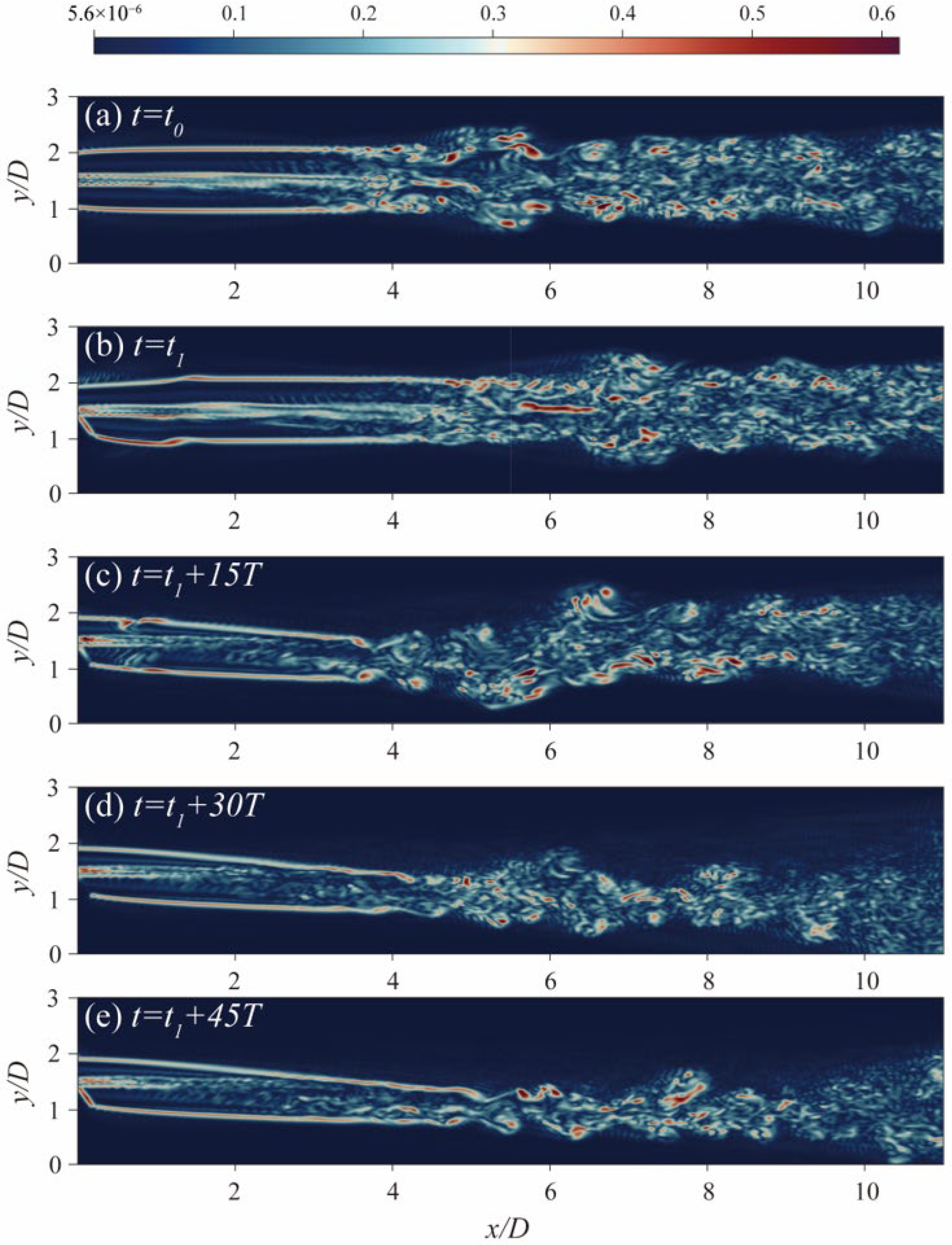
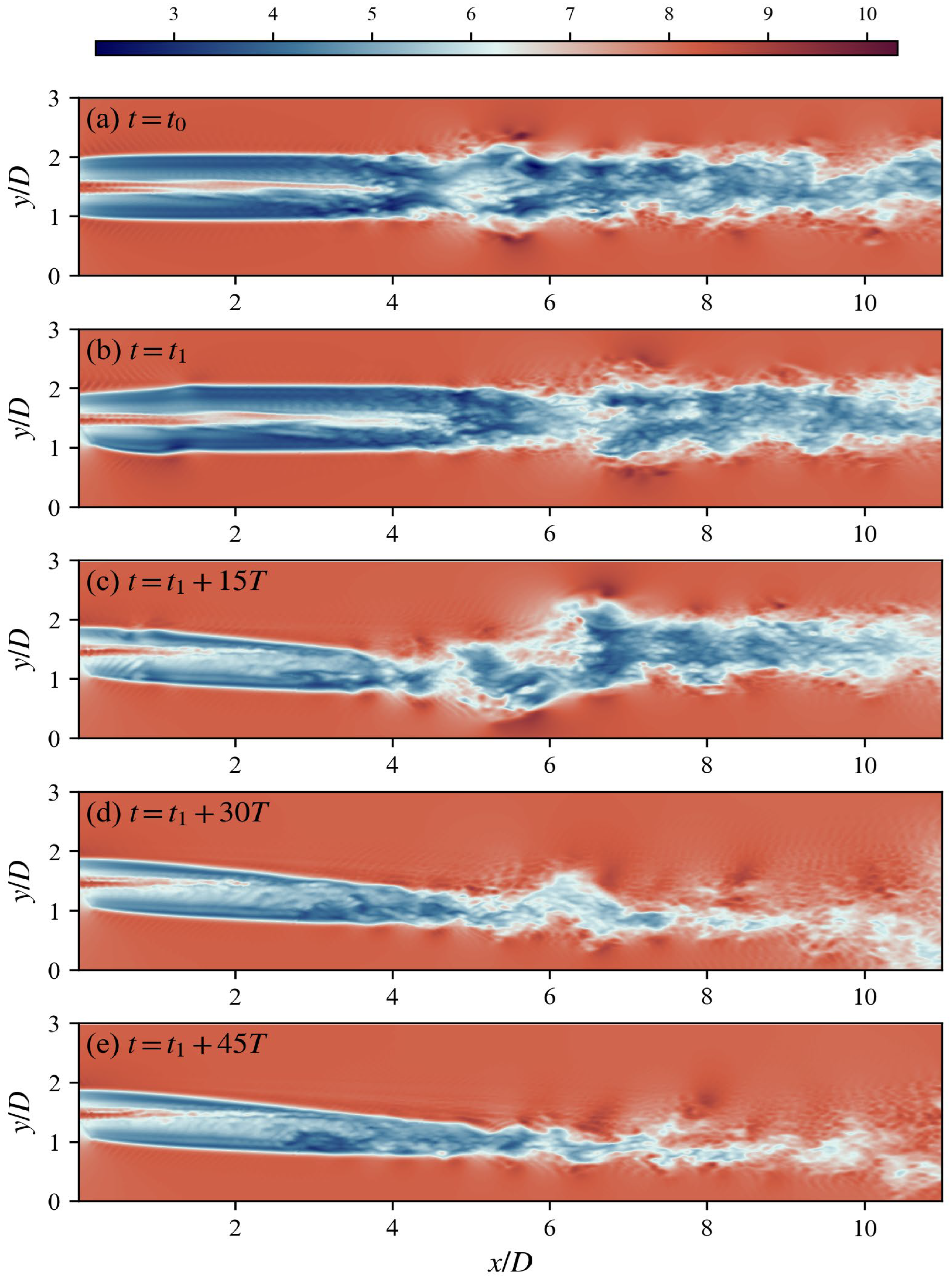
The evolution of the streamwise velocity field, shown in Figure 5, provides the clearest evidence of yaw-induced wake steering. At the initial moment t = t 0 , when the turbine is aligned with the free-stream flow, the wake is symmetric and stable. A well-defined velocity deficit core extends downstream along the centerline, with limited lateral distortion. The near wake maintains high coherence, dominated by the rotor-induced momentum deficit, whereas the far wake shows gradual velocity recovery due to entrainment of ambient flow.
Once yawing is initiated at t = t 1 , a distinct lateral displacement of the velocity deficit core emerges. The wake begins to bend toward the negative y -direction as a result of the lateral thrust component generated by the yawed rotor. This phenomenon is physically linked to the deflection of the rotor loading distribution: when the rotor plane is misaligned, the incoming flow impinges at an angle, producing asymmetric pressure loading across the disk. The higher pressure on the windward side pushes the wake laterally, resulting in a measurable deflection angle.
Between t = t 1 + 15 T , and t = t 1 + 30 T , the wake deflection intensifies, and the wake core becomes narrower. This narrowing is caused directly by increased activity in the shear layer along the wake boundary. The deflection of flow creates an asymmetric velocity gradient between the wake and the outer field and permits more efficient momentum exchange. A high-speed region near the inflection point is seen and indicates elevated mixing at the shear interface. There is some undulation along the wake boundary, and this indicates the creation of shear-layer instabilities that may trigger vortex roll-up.
At t = t 1 + 45 T , the wake reaches a quasi-steady deflected state. The lateral displacement no longer increases significantly, showing that the wake has adapted to the new operating condition. The velocity deficit recovers faster downstream than in the aligned case, showing that yaw not only deflects the wake but also improves recovery by augmenting entrainment. This faster recovery has significant implications for downstream turbines, as it can help alleviate power losses and unsteady loading in wind farms.
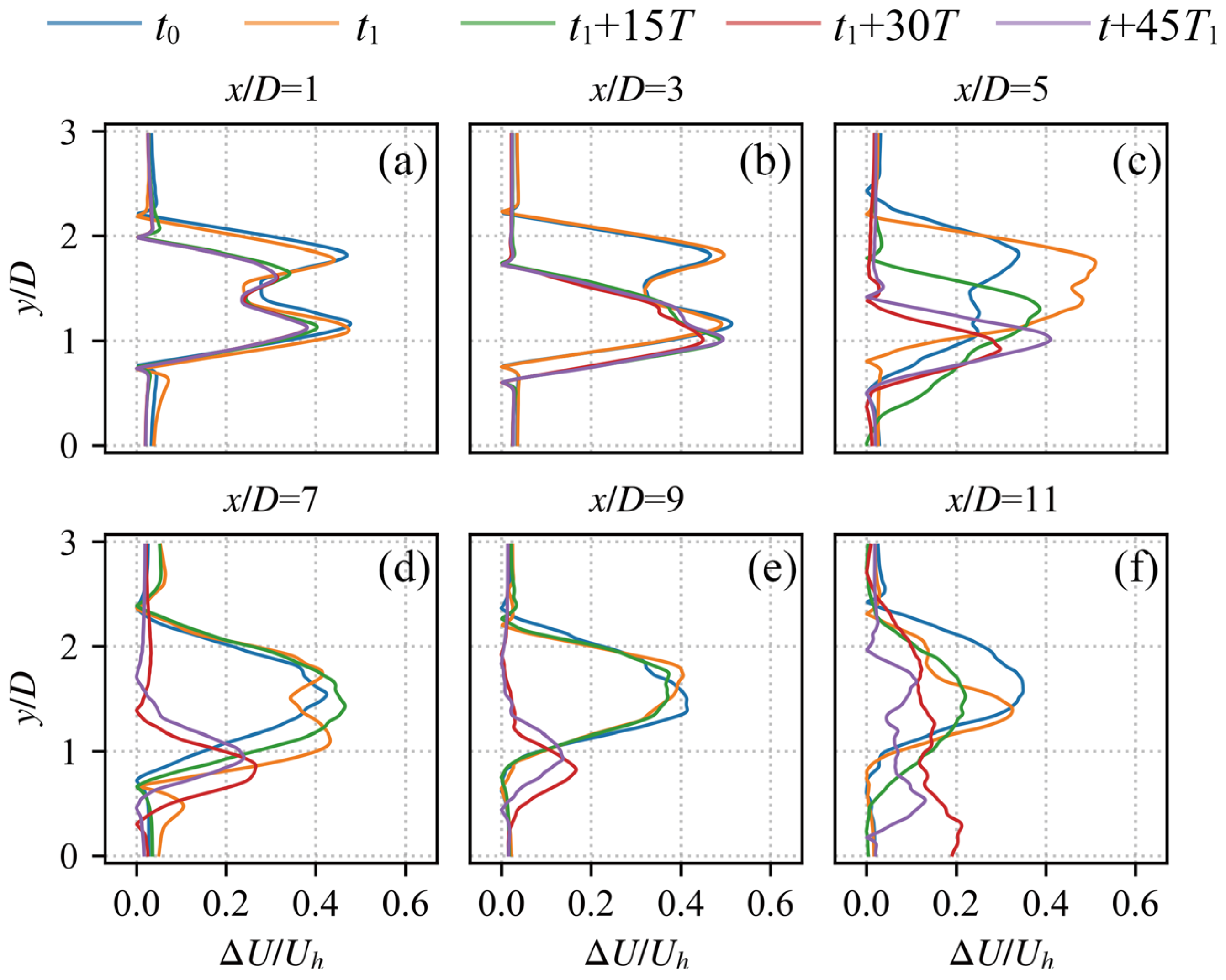
To quantify these trends, velocity deficit profiles are extracted at multiple downstream locations (Figure 6). In the near wake ( x / D = 1 and 3 ), the wake center remains aligned with the rotor axis, and the deficit magnitude is large, exceeding 50% of the free-stream velocity. At this stage, the convective distance is too short for yaw-induced momentum redistribution to fully manifest. The flow remains dominated by the initial momentum deficit generated at the rotor disk.
As the flow convects downstream to x / D = 5 and 7 , the wake center shifts significantly toward the negative y -direction. The velocity deficit begins to decrease and the profile shape becomes asymmetric, reflecting both lateral displacement and increased shear-layer mixing. The narrowing of the wake at this location corresponds to the stronger deflection and shear development seen earlier in the velocity contours. This region represents a transitional stage where coherent wake structures are gradually replaced by more turbulent flow.
In the far wake ( x / D = 9 and 11 ), the velocity deficit continues to weaken, and the profile spreads over a wider lateral extent. The maximum deficit decreases substantially, indicating that entrainment of external high-speed flow has replenished much of the momentum deficit. Notably, the recovery is faster on the yawed side, illustrating the anisotropic nature of the flow. This effect is essential for wake control strategies, as it enables partial mitigation of wake impacts on downstream turbines by steering the wake away from their rotor area and enhancing re-energization. Interestingly, yawed side recovery is faster, which indicates anisotropy of the flow. This effect is critical in wake control methods as it can facilitate partial wake reduction in effects on downstream turbines by bending the wake away from their rotor area and inducing re-energization.

3.1.2. Spanwise Velocity Field

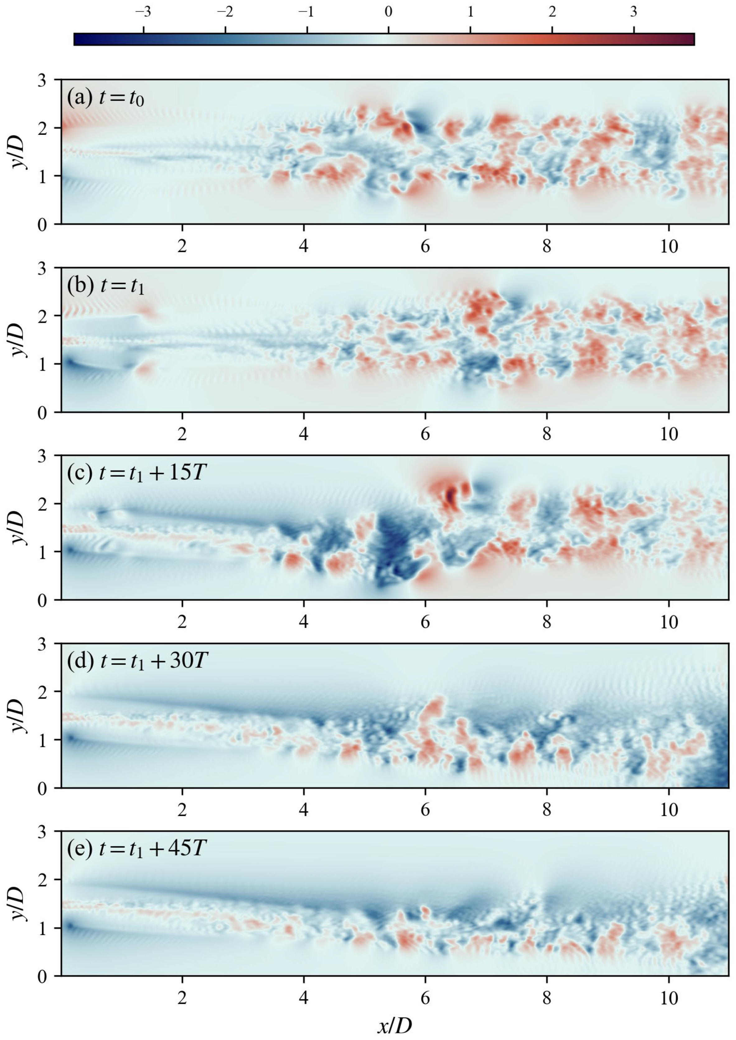
The spanwise velocity field (Figure 7) provides additional insight into the cross-flow dynamics responsible for wake steering. In the baseline aligned case ( t = t 0 ), spanwise velocities are weak and symmetrically distributed, indicating the absence of significant lateral momentum flux. The wake is essentially two-dimensional in its large-scale structure.
Once yaw is introduced, the situation changes drastically. At t = t 1 , a pronounced spanwise velocity gradient form on the leeward side of the rotor, revealing the presence of lateral shear. This shear-layer is a key driver of wake deflection: by generating cross-stream momentum flux, it pushes the wake core away from the turbine axis. As the wake evolves ( t = t 1 + 15 T to t = t 1 + 30 T ), alternating regions of positive and negative spanwise velocity emerge and intensify. This pattern indicates the roll-up of the shear layer and the formation of secondary vortices that enhance mixing between the wake and ambient flow.
At t = t 1 + 45 T , the spanwise flow weakens slightly as the wake stabilizes into its deflected trajectory. However, lateral transport remains clearly visible, confirming that the deflected wake is maintained by persistent cross-flow momentum exchange. This mechanism is crucial for understanding the sustained steering effect under steady yaw operation.
To quantify the yaw-induced asymmetry, the instantaneous velocity field was phase-averaged over several rotor revolutions and the wake-center location was identified using the minimum axial-velocity criterion. Figure 6 illustrates the lateral displacement of the wake centerline yc(x) for both aligned and yawed cases. In the yawed configuration, the wake deflection increases almost linearly up to x / D ≈ 4 and then gradually saturates, consistent with previous field observations by Fleming et al. [38]. The maximum lateral offset reaches approximately 0.28 D at 6 D downstream, corresponding to an effective deflection angle of ≈18°.Quantitatively, the wake center deflection is measured as y / D = 0.12 at x / D = 3, y/D = 0.21 at x / D = 5, and y/D = 0.28 at x / D = 6, confirming a near-linear deflection trend in the near-wake region before saturation.

3.1.3. Vorticity Magnitude Field

The vorticity vector is defined as   ω = × u , and its magnitude is computed as:
ω = w y v z 2 + u z w x 2 + v x u y 2  
where   u , v , and w are the streamwise, spanwise, and vertical velocity components, respectively.
The vorticity magnitude field shown in Figure 8 captures the dynamics of coherent structures that drive mixing and entrainment. At t = t 0 , the near wake is characterized by strong tip vortices shed from the blade tips and a coherent hub vortex along the centerline. These structures are stable and aligned, resulting in a relatively smooth and symmetric wake evolution.
When yawing starts at t = t 1 , asymmetry develops between the windward and leeward sides of the wake. Vortex strength decreases on the leeward side due to altered loading, and small disturbances appear near the shear layer. Over time ( t = t 1 + 15 T to t = t 1 + 30 T ), these disturbances amplify, leading to vortex stretching, deformation, and eventual breakdown. This transition from coherent to turbulent vortex structures is accompanied by a marked increase in shear-layer mixing, consistent with the velocity field observations.
By t = t 1 + 45 T , large-scale vortical structures have largely disintegrated into fine-scale turbulence. This enhanced turbulence intensity plays a decisive role in the rapid wake recovery observed downstream. Physically, vortex breakdown increases the effective mixing layer thickness, enabling faster entrainment of ambient kinetic energy into the wake core. This process not only restores the momentum deficit more efficiently but also reduces wake persistence, making wake steering a powerful tool for wind farm optimization.
The normalized velocity-deficit profiles (Figure 7) further show that yaw motion accelerates wake recovery beyond x / D = 5. The mean velocity deficit at 6D is reduced by 24% relative to the aligned case, indicating enhanced entrainment and turbulence mixing caused by cross-flow shear. The lateral shear layer on the deflected side exhibits elevated Reynolds stresses, which contribute to faster momentum exchange between the wake core and ambient flow. These findings highlight the two-stage recovery behavior typical of dynamically yawed wakes: an initial rapid deflection phase dominated by large coherent structures, followed by gradual re-symmetrization driven by ambient turbulence.

3.2. POD Analysis of Pre-Yaw Wake

As described in Section 2.5, Proper Orthogonal Decomposition (POD) was applied to 200 velocity snapshots from the pre-yaw steady-state simulation to establish a baseline for coherent wake structures. This reference case enables direct comparison with the yawed wake and isolates the aerodynamic effects of active yaw control.

3.2.1. POD Energy Distribution

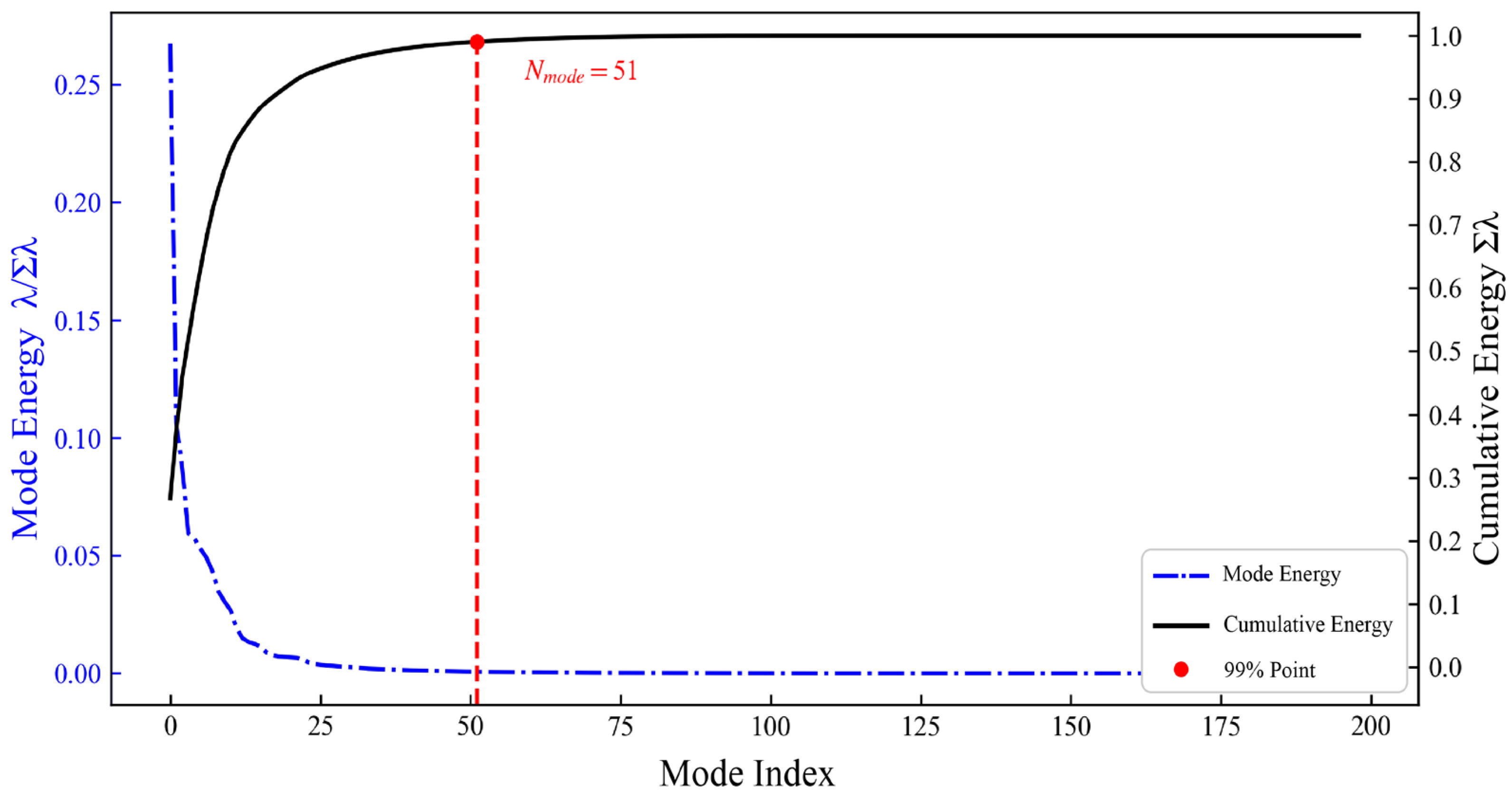
The distribution of energy among the first 200 POD modes is illustrated in Figure 9. A striking feature of the spectrum is the dominance of the first few modes. Mode 1 alone contains about 26.7% of the total kinetic energy, while Modes 2 and 3 account for 10.6% and 8.7%, respectively. In other words, nearly half of the entire flow energy is captured by just three modes. Beyond these, the energy content drops sharply. By Mode 25, approximately 94% of the total energy has been accumulated, and at Mode 51, the cumulative energy reaches 99%.
This behavior is typical of wind turbine wakes in uniform inflow and confirms that the wake is governed by a number of large-scale dominant flow structures. The ubiquitous dominance of these large coherent motions, namely wake meandering and tip vortex behavior, suppresses the relative contribution of small-scale turbulence. Previous POD studies of turbine wakes, also observed similar patterns, underscoring the low-dimensional nature of these flows.
Practically, the rapid convergence of energy has profound implications. Since the major fraction of the flow energy is concentrated within a few modes, it is possible to reconstruct or predict the wake accurately by retaining just the principal modes. This significantly reduces the computation cost compared to interacting with the full three-dimensional time-dependent field. In the context of the management of the wind farm, these reduced-order models would be of great help for fast wake prediction, the developmental study of flow control algorithms, and exploration of optimization studies.
The wake-deflection dynamics can also be characterized by the instantaneous power-spectral density of velocity fluctuations at selected downstream locations as shown in Figure 8. A dominant frequency corresponding to a Strouhal number St ≈ 0.18 is observed, matching the global wake-meandering mode reported in wind-tunnel measurements. The amplitude of this mode decreases after the yaw motion ends, implying that large-scale unsteadiness decays as the wake reaches its quasi-steady deflected state.

3.2.2. Spatial Structures of Dominant Modes

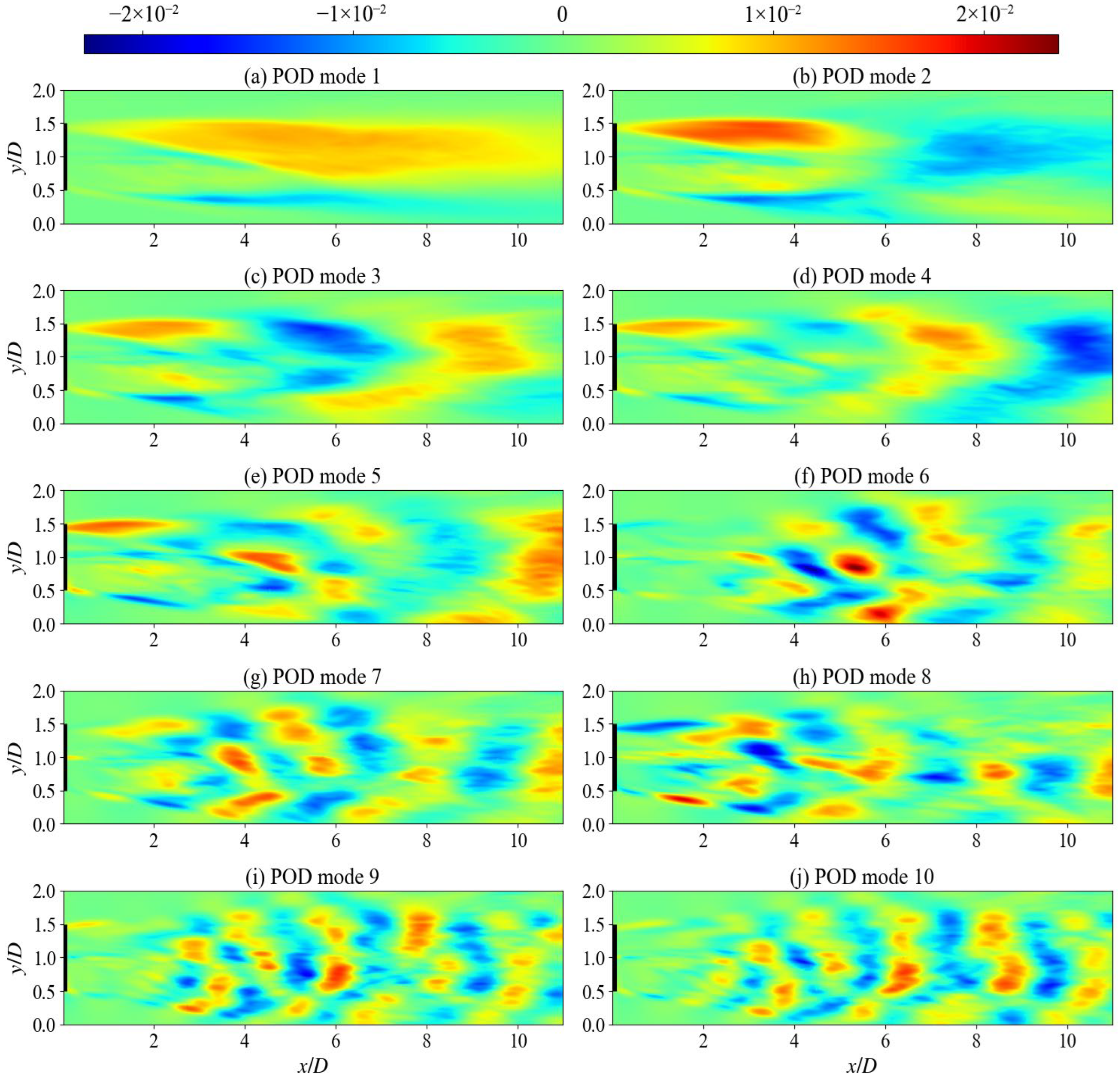
The first ten POD modes are presented in Figure 10, as they capture the dominant coherent structures governing wake meandering and shear-layer dynamics. Modes beyond the 10th order are typically higher harmonics of the leading modes, exhibiting similar spatial patterns at higher frequencies but lacking distinct physical uniqueness, and thus contribute minimally to the fundamental wake physics. Retaining the first 10 modes ensures that the primary flow features are resolved while enabling a consistent basis for comparison with the yawed case.
Mode 1 is characterized by two large-scale lobes symmetric with respect to the rotor axis in the near wake. Farther downstream, these merge into a broad, slowly varying structure that spans much of the lateral domain. This behavior is typical of wake meandering, a low-frequency oscillation of the wake core that strongly influences downstream turbine performance and loading. Modes 2 and 3 also display large-scale structures, particularly near the wake boundary, but they are superposed with smaller fluctuations close to the centerline. These finer features likely correspond to root vortex interactions or tower-shedding effects. Their spatial distribution suggests that they act as a bridge between global wake deflection and local shear-layer instabilities.
Modes 4 and 5, as well as Modes 6 and 7, appear as mode pairs with nearly identical energy levels but mirrored spatial patterns. This is a well-known signature in POD of traveling wave-like structures or periodic phenomena. In this context, the paired modes are associated with Kelvin–Helmholtz (K–H) shear-layer instabilities, which develop along the interface between the wake and the freestream. These instabilities promote mixing and are central to wake recovery. Modes 6 and 7 in particular show clear periodic streaks aligned in the streamwise direction—a classic indicator of vortex roll-up. These structures drive entrainment of high-momentum freestream air into the wake core, accelerating its re-energization.
Mode 8 maintains a similar shape but with smaller scales and weaker intensity, hinting at higher-frequency components of the same instability mechanism. Modes 9 and 10 exhibit smaller, more irregular structures concentrated around the tip vortex region and near the centerline. These patterns signal the onset of vortex breakdown and the transition to turbulence. Even though they contribute less energy individually, they are crucial for triggering the small-scale mixing processes that eventually dominate in the far wake.
Altogether, the modal structures reveal an unmistakable physical hierarchy. The early modes (1–3) almost exclusively describe the long, low-frequency motions governing the overall displacement of the wake, such as meandering. Modes within the intermediate range (around 4–8) are associated with shear-layer breakup and the generation of vortical motions along the wake perimeter. Finally, the higher modes (9–10) summarize the higher-chaos, fine-scale turbulent motions responsible for the breakup of the tip vortices and transformation toward fully developed turbulence downstream.

3.2.3. Interpretation

The POD analysis identifies the non-yaw wake as consisting of a few energetic, long-scale coherent structures, with Mode 1 retaining the slow longitudinal motion of the whole wake and the rest of the modes, the latter of which denote paired modes, signifying shear-layer instabilities. These structures govern the momentum transport and the whole wake evolution. The fast energy dissipation reinforces the notion that even though the flow appears complex, the inherent dynamics are actually low-dimensional.
The pre-yaw wake is highly low-dimensional: the first 3 modes capture 46.0% of the total kinetic energy, and 99% is captured by just 51 modes. This quantifies the dominance of large-scale meandering and confirms that a reduced-order model using <60 modes can faithfully reconstruct the baseline wake.

3.3. POD Analysis of Yawing Wake

To investigate how yaw control alters the coherent structures and energy distribution within the wake, Proper Orthogonal Decomposition (POD) was applied to the velocity field during the yaw maneuver. Unlike the baseline non-yawed case, the yawing process introduces a number of new phenomena: transient flow evolution, lateral asymmetry, enhanced mixing, and increased turbulence intensity. These effects modify both the energy distribution across POD modes and the structure and dynamics of the coherent flow patterns.

3.3.1. POD Energy Distribution

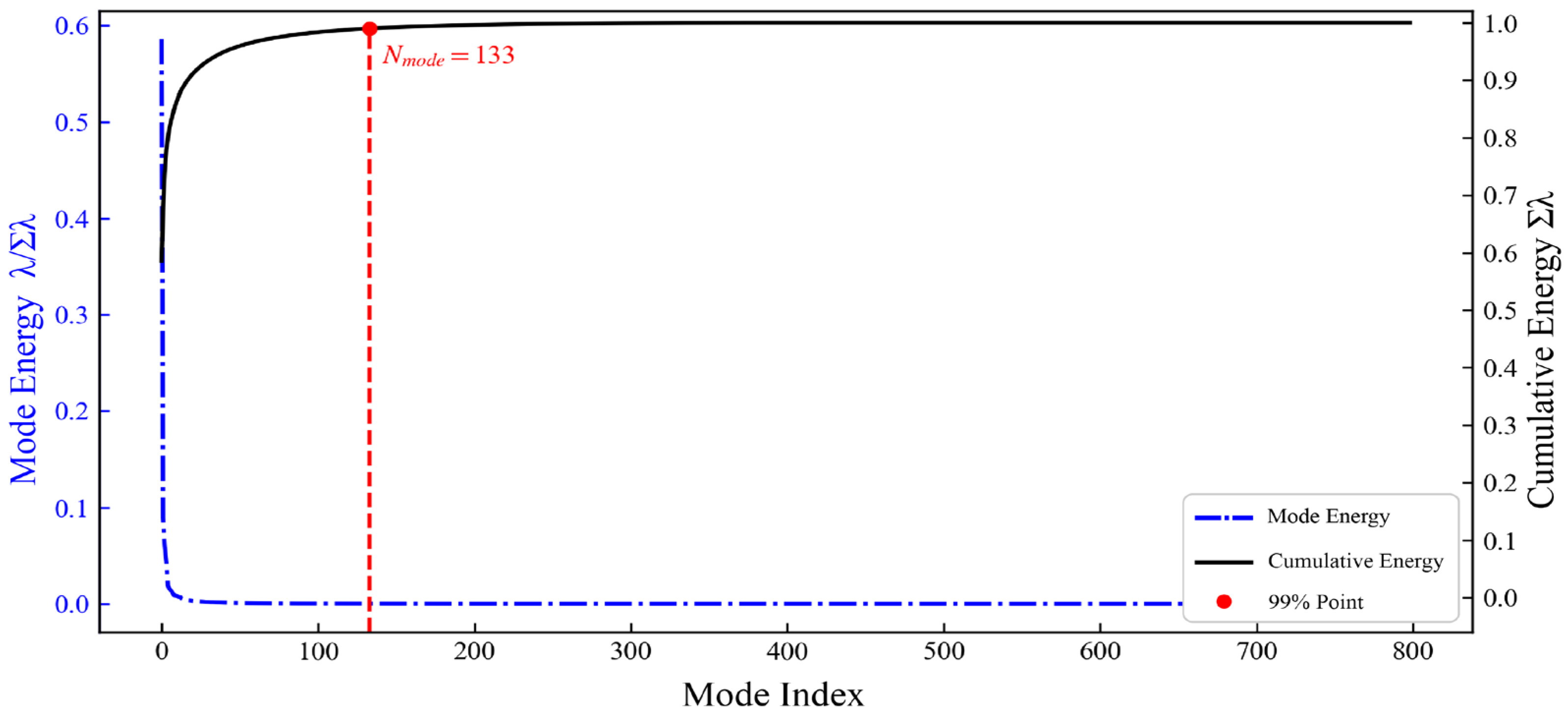
The modal energy spectrum for the yawing wake is presented in Figure 11. Compared with the non-yaw case, the energy is distributed more broadly, reflecting a more complex flow state. The first few modes capture a smaller portion of the total energy, and the decay of modal energy with increasing mode number is noticeably slower. The cumulative energy reaches 99% at the 133rd mode, which is substantially higher than the 51 modes needed in the aligned inflow condition.
This expanded spectrum is a direct manifestation of yaw-induced unsteadiness. By imposing a yaw angle, the rotor generates lateral velocity components and disturbs the shear layers, triggering additional coherent structures throughout the wake. As a result, the flow dimensionality increases: more modes are required to accurately reconstruct the velocity field. This behavior reflects the combined influence of wake deflection, vortex deformation, and shear-layer instabilities that become active as the wake adjusts to the yawed inflow.

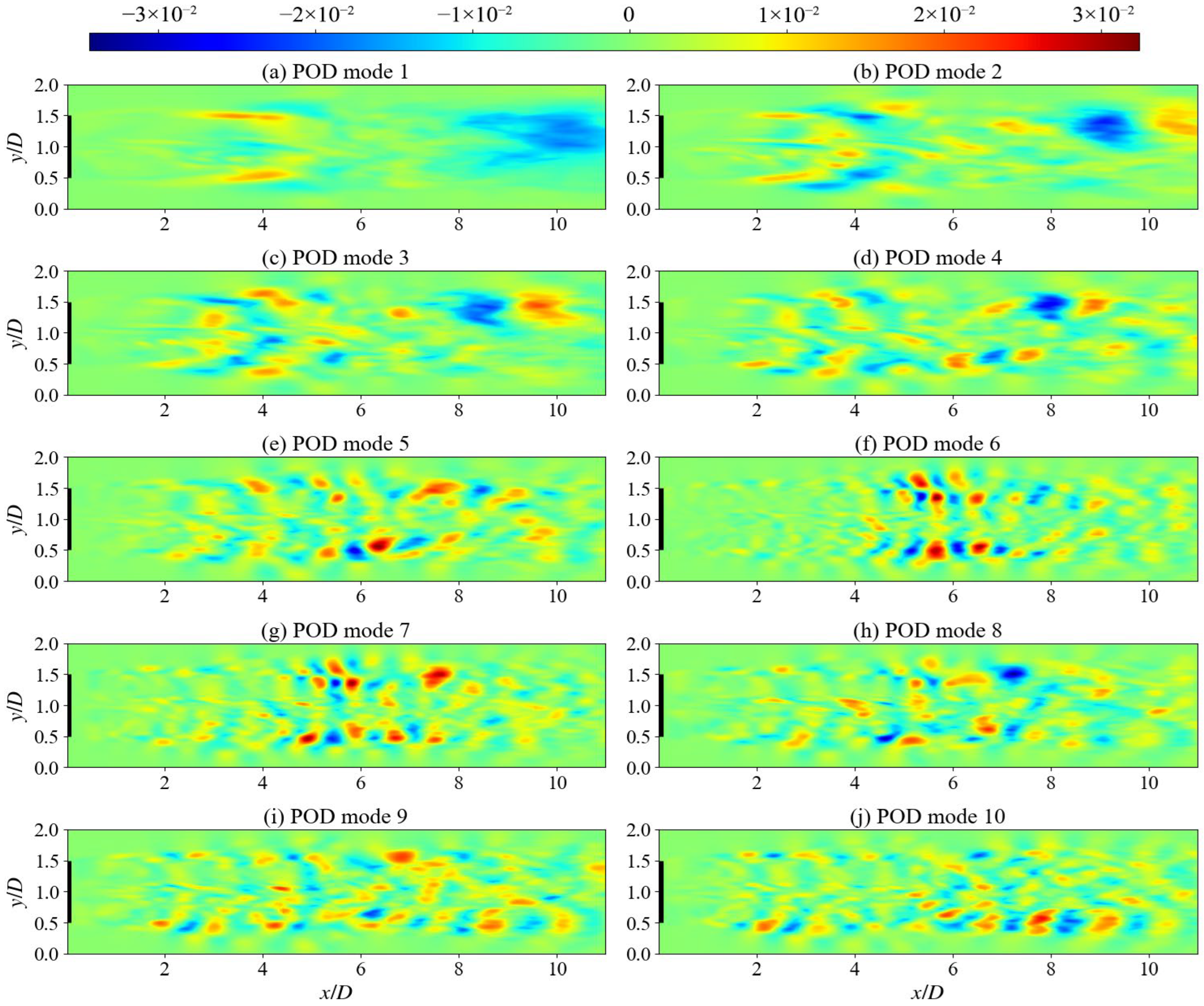
3.3.2. Spatial Structures of Dominant Modes

The spatial structures of the first ten POD modes are shown in Figure 12, as they represent the most physically relevant coherent motions during the transient yaw maneuver. Higher-order modes (>10) generally correspond to harmonic content or fine-scale noise without independent dynamical significance, and are therefore omitted for clarity. This truncation aligns with standard practice in modal analysis of turbine wakes and ensures a direct, physically meaningful comparison with the pre-yaw baseline.
Modes 2–4 have significant action within the area of the shear layers and the nacelle region. In comparison to their analogous modes of the non-yawed wake, the current modes are far more asymmetric and irregular, and therefore emphasize the stronger shear-layer instabilities caused by yaw. These are the responsible mechanisms injecting energy into the smaller scales and amplifying turbulent mixing strongly.
Modes 5–7 exhibit periodic patterns localized on the shear layer and extending into the far wake. These are the signatures of Kelvin–Helmholtz vortex roll-up, and they serve as the link between the large-scale coherent structures and the turbulent fluctuations of the higher frequencies. This process facilitates the momentum entrainment from the freestream towards the wake, and this accelerates the recovery.
The upper modes (8–10) have finer, more dispersed structures spread throughout the wake cross-section. These modes are picking up the fine-scale, high-frequency motions that are present as the wake goes through the early transient yawing stage into a new deflected quasi-steady regime. Their existence reinforces the idea that yawing adds to the spatial complexity of the wake, creating extra vortical structures on multiple scales.

3.3.3. Temporal Evolution of POD Coefficients

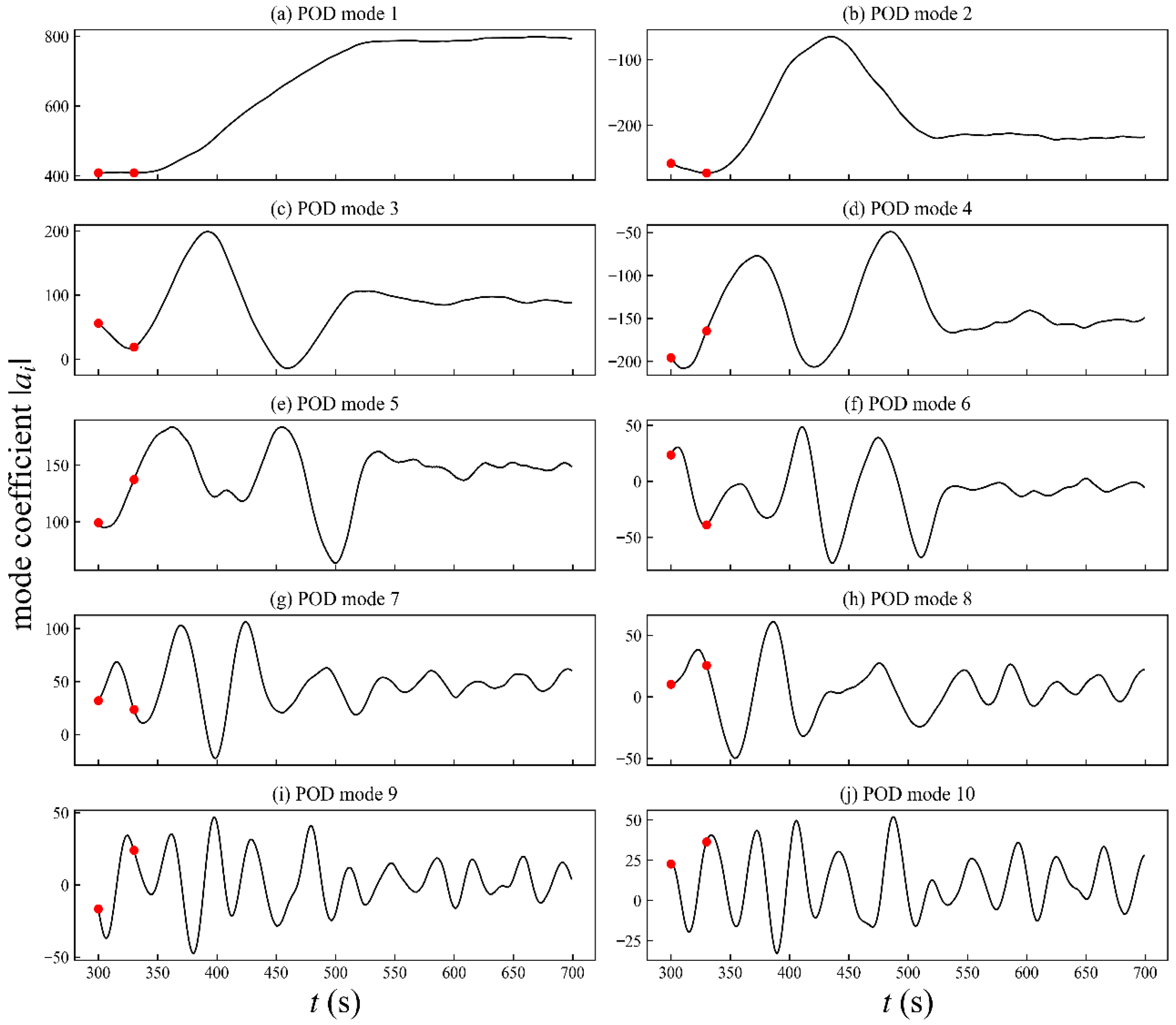
Figure 13 plots the time evolution of the modes corresponding to the first ten modes. This time series analysis provides additional insight into the way flow structures respond to yawing.
At the initial stage of the yaw motion (t = t1), amplitudes of Mode 2–8 see a substantial growth, suggesting rapid formation of unsteady structures of the shear layer and the near-wake region. With the proceeding yaw rotation and eventual settling, these modes reach a plateau, which, by analogy, points towards the transition of the flow towards a new equilibrium related to the modified wake regime. Interestingly, the time scales of stabilization of these modes match the temporal evolution of Mode 1 well, evidencing that both the big-scale and the intermediate structures adapt on similar time scales.
In contrast, Modes 9 and 10 exhibit markedly different characteristics. They display continuous, high-frequency oscillatory behavior during the yawing process, lacking any discernible stabilization trend. These variations are linked to fine-scale turbulence and demonstrate greater sensitivity to disturbances in the shear layer. Even once the large-scale flow attains a stable deflected configuration, these modes persist in their fluctuations, underscoring the ongoing presence of small-scale turbulence in the far wake.

3.3.4. Interpretation

The POD analysis shows how yaw redistributes turbulent energy across different scales. While the first three modes capture 46.0% of the total kinetic energy in the pre-yaw wake, they account for only 36.2% under yaw, a 21% relative reduction in large-scale coherence. As a result, 133 modes are required to reach 99% energy capture during yaw, compared to just 51 modes in the aligned case. This confirms that yaw increases flow dimensionality by energizing small-scale, high-frequency structures. As shown in Figure 12, the low-order modes (1–3) stabilize within 2–3 rotor periods after yaw completion, while the higher-order modes (>8) remain active for much longer, sustaining elevated turbulence that drives wake recovery.
In summary, the energy distribution shifts from being concentrated in a limited number of modes; rather, it disperses across a broader array, indicating an elevation in both dimensionality and complexity of the flow. The temporal evolution of the POD modes also demonstrates this shift. Lower-order modes, associated with the global displacement and meander of the wake, become stabilized comparatively rapidly once the rotor has completed yawing. However, higher-order modes are active for orders of magnitude longer, and they are responsible for resolving the long-lasting turbulent motions governing the far wake. This interplay of big-scale deflection and small-scale turbulence has immediate effects on wake steering approaches, downstream loading of turbines, and the design of active control systems of wind farms.

4. Conclusions

This study has quantified the transient wake dynamics of an NREL 5 MW offshore wind turbine under active yaw control by coupling high-fidelity large-eddy simulation with time-resolved proper orthogonal decomposition. The results demonstrate that a 25° yaw maneuver induces a lateral wake deflection of 0.28 D at 6 D downstream and accelerates velocity recovery by 24% compared to the aligned case, evidence of enhanced momentum replenishment through intensified turbulent mixing.
POD analysis reveals a fundamental shift in the spectral organization of the wake. While the pre-yaw wake is governed by a low-dimensional set of coherent structures, requiring only 51 modes to capture 99% of the kinetic energy, the yawed wake exhibits a marked increase in flow dimensionality, necessitating 133 modes for equivalent energy representation. This broadening of the modal energy spectrum reflects the breakdown of large-scale coherence into a richer hierarchy of small-scale turbulent motions, driven by shear-layer asymmetry and vortex destabilization.
Critically, the temporal evolution of POD modes uncovers a multi-timescale relaxation process. Low-order modes (1–3), which encode the global wake deflection and meandering, stabilize within 2–3 rotor periods after yaw completion. In contrast, higher-order modes (>8), associated with fine-scale turbulence in the shear layer, remain active far longer, sustaining elevated mixing that drives continued wake recovery well beyond the geometric reorientation phase. This separation of timescales explains why wake steering strategies based solely on steady-state deflection may underestimate the full aerodynamic benefit of yaw: the enhanced turbulence persists even after the wake appears quasi-steady, providing a prolonged window of improved re-energization.
These findings underscore that yaw control is not merely a geometric redirection tool but an active turbulence generator that reshapes the entire wake energy cascade. For wind farm operation, this implies that optimal yaw protocols must account for both the immediate deflection and the delayed decay of small-scale turbulence. Future control strategies could leverage this dual mechanism, using early-time deflection to avoid downstream rotors while exploiting late-time mixing to accelerate recovery, thereby maximizing energy capture while mitigating fatigue loads in offshore arrays.

Author Contributions

Conceptualization, O.S. and L.W.; methodology, O.S., B.Z. and J.G.; software, O.S.; validation, O.S., B.Z. and J.G.; formal analysis, O.S.; investigation, O.S. and B.Z.; writing—original draft preparation, O.S.; writing—review and editing, O.S., B.Z., J.G. and L.W.; supervision, L.W. All authors have read and agreed to the published version of the manuscript.

Funding

The authors acknowledge the support of this research from the National Natural Science Foundation of China (Grant No. 12002137), Postdoctoral Science Foundation of Jiangsu Province (Grant No. 2021K110B), China Postdoctoral Science Foundation (Grant No. 2023M742935).

Data Availability Statement

The data presented in this study are available on request from the corresponding author due to ongoing related research projects.

Acknowledgments

The first author wishes to convey profound appreciation to the supervisor for their unwavering leadership, insightful input, and invaluable support during this research endeavor. Gratitude is also expressed to the research group members for their valuable discussions, technical support, and encouragement throughout the simulation and analytic stages of this study. The computational resources and academic environment provided by the university have played an essential role in the successful completion of this study. Finally, the author is deeply grateful to family and friends for their patience, understanding, and constant encouragement.

Conflicts of Interest

Author Jie Ge was employed by the company Shimge Pump Industry (Zhejiang) Co., Ltd. The remaining authors declare that the research was conducted in the absence of any commercial or financial relationships that could be construed as a potential conflict of interest.

Nomenclature and Abbreviations

Nomenclature
SymbolDescriptionUnit
D Rotor diameter m
U Free-stream velocity m   s 1
ω Vorticity vector ω = × u s 1
τ i j Subgrid-scale stress tensor m 2 s 2
C s Smagorinsky constant
Δ Grid filter width, Δ = Δ x Δ y Δ z 1 3 m
s ¯ i j Resolved strain-rate tensor s 1
z 0 Surface roughness length m
λ k POD eigenvalue, energy of mode k
T Rotor rotation period s
u Velocity vector m   s 1
u , v , w Velocity fluctuations m   s 1
x , y , z Streamwise, spanwise, and vertical coordinates m
Abbreviations
LESLarge-Eddy Simulation
PODProper Orthogonal Decomposition
ALMActuator Line Model
IBMImmersed Boundary Method
ABLAtmospheric Boundary Layer
SGSSub-Grid Scale
CFLCourant–Friedrichs–Lewy
TSRTip-Speed Ratio
TKETurbulent Kinetic Energy
NRELNational Renewable Energy Laboratory

References

  1. GWEC. Global Wind Report 2024; Global Wind Energy Council: Brussels, Belgium, 2024. [Google Scholar]
  2. Dai, Y.; He, K.; Li, B.; Zhai, M. Influence of double-fork blade tip structure on wind turbine vibration. J. Drain. Irrig. Mach. Eng. 2022, 40, 276–281. [Google Scholar]
  3. Du, Y.; Wang, J.; Wang, Y.; Zhang, J.; Yan, S. Effect of wind direction changing speed on power and speed of wind turbine. J. Drain. Irrig. Mach. Eng. 2023, 41, 167–172. [Google Scholar]
  4. Guo, T.; Li, Y.; Li, D.; Wei, H.; Li, R. Influence of dynamic wind direction on evolution law of wind turbine wake. J. Drain. Irrig. Mach. Eng. 2023, 41, 1255–1260. [Google Scholar]
  5. Gao, W.; Zhang, L.; Yao, H.; Yan, R. Vortex characteristics of horizontal axis wind turbine blade and wake flow field based on dynamic mesh. J. Drain. Irrig. Mach. Eng. 2023, 41, 173–179. [Google Scholar]
  6. Dai, Y.; Guo, C.; Li, B.; Jiang, J.; Wang, C. Influence of centrifugal force and aerodynamic load on strain characteristics of wind turbine blades. J. Drain. Irrig. Eng. 2023, 41, 576–582. [Google Scholar]
  7. Stevens, R.J.A.M.; Meneveau, C. Flow structure and turbulence in wind farms. Annu. Rev. Fluid Mech. 2017, 49, 311–339. [Google Scholar] [CrossRef]
  8. Meyers, J.; Meneveau, C. Optimal turbine spacing in fully developed wind farm boundary layers. Wind Energy 2012, 15, 305–317. [Google Scholar] [CrossRef]
  9. Barthelmie, R.J.; Jensen, L.E. Evaluation of wind farm efficiency and wind turbine wakes at the Nysted offshore wind farm. Wind Energy 2010, 13, 573–586. [Google Scholar] [CrossRef]
  10. Bastankhah, M.; Porté-Agel, F. A new analytical model for wind-turbine wakes. Renew. Energy 2014, 70, 116–123. [Google Scholar] [CrossRef]
  11. Le, K.; Yu, Y.; Wang, Y.; Wu, C.; Wang, Q.; Luo, K.; Fan, J. Atmospheric stability based on mesoscale simulations and its impact on operational characteristics of wind farms. J. Drain. Irrig. Mach. Eng. 2025, 43, 87–93. [Google Scholar]
  12. Li, Y.; Ma, Y.; Tong, G.; Yang, S.; Xiao, Z. Numerical simulation of starting performance of vertical axis wind turbine with B-Spline curve wind gathering devices. J. Drain. Irrig. Mach. Eng. 2024, 42, 265–272. [Google Scholar]
  13. Sanderse, B.; van der Pijl, S.P.; Koren, B. Review of computational fluid dynamics for wind turbine wake aerodynamics. Wind Energy 2011, 14, 799–819. [Google Scholar] [CrossRef]
  14. Li, Y.; Tong, G.; Qu, C.; Feng, F. Numerical simulation of aerodynamic characteristics of straight-bladed vertical axis wind turbine with large solidities. J. Drain. Irrig. Mach. Eng. 2022, 40, 701–706. [Google Scholar]
  15. Porté-Agel, F.; Bastankhah, M.; Shamsoddin, S. Wind-turbine and wind-farm flows: A review. Bound.-Layer Meteorol. 2020, 174, 1–59. [Google Scholar] [CrossRef]
  16. Abkar, M.; Porté-Agel, F. Influence of atmospheric stability on wind-turbine wakes: A large-eddy simulation study. Phys. Fluids 2015, 27, 035104. [Google Scholar] [CrossRef]
  17. Yuan, J.; Gao, Q.; Wang, L.; Wang, Z. Analysis and optimization on aerodynamic acoustic characteristics of multi-blade centrifugal fan for bathroom heaters. J. Drain. Irrig. Mach. Eng. 2025, 43, 795–802. [Google Scholar]
  18. Berkooz, G.; Holmes, P.; Lumley, J.L. The proper orthogonal decomposition in the analysis of turbulent flows. Annu. Rev. Fluid Mech. 1993, 25, 539–575. [Google Scholar] [CrossRef]
  19. Xiao, S.; Zhu, X.; Narasimhan, G.; Gayme, D.F.; Meneveau, C. Wind farm dynamics over a diurnal cycle: Analysis of a comprehensive large-eddy simulation, web-services accessible dataset. J. Renew. Sustain. Energy 2025, 17, 063301. [Google Scholar] [CrossRef]
  20. Alkhabbaz, A.; Hamza, H.; Daabo, A.; Yang, H.; Yoon, M.; Koprulu, A.; Lee, Y. The aero-hydrodynamic interference impact on the NREL 5-MW floating wind turbine experiencing surge motion. Renew. Energy 2024, 295, 116970. [Google Scholar] [CrossRef]
  21. Xie, S.; He, J.; Zhang, C.; Kan, Y.; Ma, J.; Zhang, Z. Aero-hydro-servo-elastic coupled modeling and dynamics analysis of a four-rotor floating offshore wind turbines. Ocean Eng. 2023, 272, 113724. [Google Scholar] [CrossRef]
  22. Taira, K.; Brunton, S.L.; Dawson, S.T.; Rowley, C.W.; Colonius, T.; McKeon, B.J.; Schmidt, O.T.; Gordeyev, S.; Theofilis, V.; Ukeiley, L.S. Modal analysis of fluid flows: An overview. AIAA J. 2017, 55, 4013–4041. [Google Scholar] [CrossRef]
  23. Sarmast, S.; Dadfar, R.; Mikkelsen, R.F.; Schlatter, P.; Ivanell, S.; Sørensen, J.N.; Henningson, D.S. Mutual inductance instability of the tip vortices behind a wind turbine. J. Fluid Mech. 2014, 755, 705–731. [Google Scholar] [CrossRef]
  24. Meyer Forsting, A.R.; Troldborg, N.; Gaunaa, M. The flow upstream of a wind turbine rotor and its effect on wake meandering. Wind Energy Sci. 2017, 2, 89–100. [Google Scholar]
  25. Foti, D.; Yang, X.; Sotiropoulos, F. Similarity of wake meandering for different turbine loading conditions and ambient turbulence intensities. Wind Energy 2016, 19, 1785–1803. [Google Scholar]
  26. Pope, S.B. Turbulent Flows; Cambridge University Press: Cambridge, UK, 2000. [Google Scholar]
  27. Luo, Z.; Wang, L.; Zhang, B.; Yuan, J.; Tan, A.C. From sparse sensing to physics-consistent reconstruction of unsteady wind turbine wakes towards control-oriented modeling. Energy Convers. Manag. 2026, 349, 120872. [Google Scholar] [CrossRef]
  28. Luo, Z.; Wang, L.; Fu, Y.; Yuan, J.; Xu, J.; Tan, A.C. Innovative sparse data reconstruction approaches for yawed wind turbine wake flow via data-driven and physics-informed machine learning. Phys. Fluids 2025, 37, 035158. [Google Scholar] [CrossRef]
  29. Zhang, B.; Wang, L.; Ge, J.; Luo, Z.; Yuan, J.; Wang, Z.; Xu, J. Advanced wake modeling in wind farm: A physics-informed framework with virtual LiDAR measurements. Phys. Fluids 2025, 37, 065133. [Google Scholar] [CrossRef]
  30. Wang, L.; Chen, M.; Luo, Z.; Zhang, B.; Xu, J.; Wang, Z.; Tan, A.C.C. Dynamic wake field reconstruction of wind turbine through Physics-Informed Neural Network and Sparse LiDAR data. Energy 2024, 291, 130401. [Google Scholar] [CrossRef]
  31. Luo, Z.; Wang, L.; Fu, Y.; Xu, J.; Yuan, J.; Tan, A.C. Wind turbine dynamic wake flow estimation (DWFE) from sparse data via reduced-order modeling-based machine learning approach. Renew. Energy 2024, 237, 121552. [Google Scholar] [CrossRef]
  32. Wang, L.; Chen, M.; Yuan, J. Spatiotemporal wake field reconstruction of wind turbine coupled with wind speed measurements. J. Drain. Irrig. Mach. Eng. 2025, 43, 260–267. [Google Scholar]
  33. Orlandi, P. Fluid Flow Phenomena: A Numerical Toolkit; Fluid Mechanics and Its Applications; Springer: Dordrecht, The Netherlands, 2000; Volume 55. [Google Scholar]
  34. Mittal, R.; Iaccarino, G. Immersed boundary methods. Annu. Rev. Fluid Mech. 2005, 37, 239–261. [Google Scholar] [CrossRef]
  35. Sørensen, J.N.; Shen, W.Z. Numerical modeling of wind turbine wakes. J. Fluids Eng. 2002, 124, 393–399. [Google Scholar] [CrossRef]
  36. Prandtl, L. Application of the lifting line theory. Z. Flugtech. Mot. 1929, 20, 36–40. [Google Scholar]
  37. Jonkman, J.; Butterfield, S.; Musial, W.; Scott, G. Definition of a 5-MW Reference Wind Turbine for Offshore System Development; NREL/TP-500-38060; National Renewable Energy Laboratory: Golden, CO, USA, 2009. [Google Scholar]
  38. Fleming, P.; King, J.; Dykes, K.; Simley, E.; Roadman, J.; Scholbrock, A.; Murphy, P.; Lundquist, J.K.; Moriarty, P.; Fleming, K.; et al. Initial results from a field campaign of wake steering applied at a commercial wind farm—Part 1. Wind Energy Sci. 2019, 4, 273–285. [Google Scholar] [CrossRef]
  39. Wang, J.; Zhao, Y.; Zhang, P.; Ren, B.; Yin, J. Experimental study on dynamic stress of blades with different materials under wind direction change. J. Drain. Irrig. Mach. Eng. 2024, 42, 273–281. [Google Scholar]
  40. Liu, Z.; Wang, J.; Wang, J.; Wang, Y.; Du, Y. Experimental study on influence of dynamic change of crosswind angle on strain of wind turbine blades. J. Drain. Irrig. Mach. Eng. 2023, 41, 499–504. [Google Scholar]
  41. Churchfield, M.J.; Lee, S.; Michalakes, J.; Moriarty, P.J. A numerical study of the effects of atmospheric and wake turbulence on wind turbine dynamics. J. Turbul. 2012, 13, N14. [Google Scholar] [CrossRef]
  42. Orlandi, P.; Leonardi, S. DNS of turbulent channel flow with two- and three-dimensional roughness. J. Turbul. 2006, 7, N73. [Google Scholar] [CrossRef]
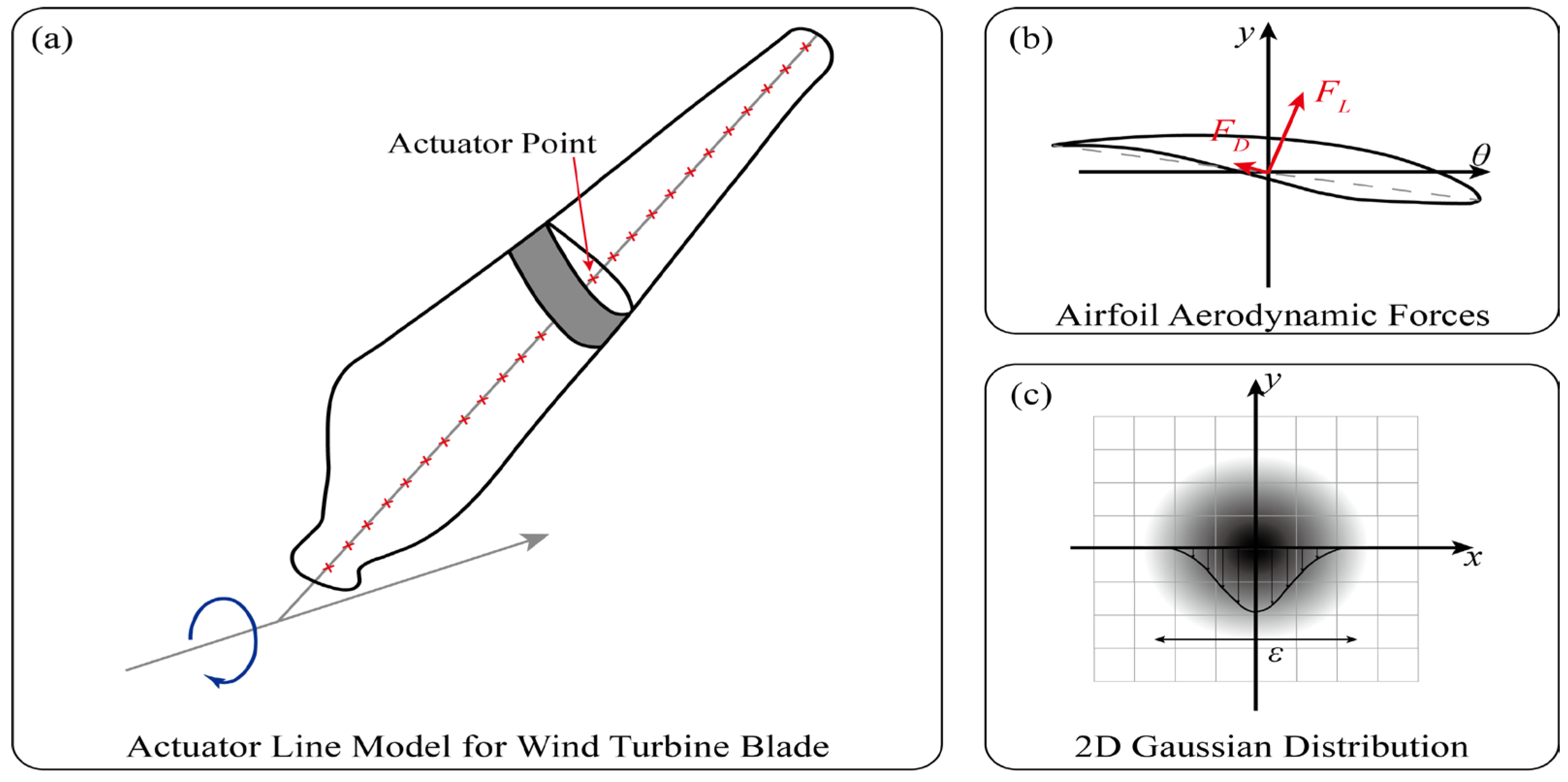
Figure 1. The diagram of Actuator Line Model. (a) the discrete blade elements, (b) the calculation of body force for each element, (c) the projection of body force to mesh grids.
Oceans 07 00025 g001
Figure 2. Computational domain and mesh configuration for LES of wind turbine wake under uniform inflow: (a) schematic of domain dimensions and coordinate system; (b) plan view showing refined Region II around the rotor (red line indicates the wind turbine rotor); (c) 3D mesh visualization and hub-height slice indicating turbine location.
Oceans 07 00025 g002
Figure 3. The temporal variation in yaw angle and selected time instants for analysis.
Oceans 07 00025 g003
Figure 4. Normalized wake velocity deficit profiles at downstream locations of 1D, 3D, and 5D. Shaded regions indicate ±1σ statistical uncertainty from time-averaging (N = 200 snapshots). The Pearson correlation coefficient between simulation and reference data is r = 0.985.
Oceans 07 00025 g004
Figure 5. Snapshots of streamwise velocity field at different time instants at the hub height level of the wake ( x / D = 0 denotes rotor plane).
Oceans 07 00025 g005
Figure 6. Wake deficit profiles at the hub height level with different streamwise distances: (a) x / D = 1 , (b) x / D = 3 , (c) x / D = 5 , (d) x / D = 7 , (e) x / D = 9 , (f) x / D = 11 .
Oceans 07 00025 g006
Figure 7. Snapshots of spanwise velocity field at different time instants at the hub height level of the wake ( x / D = 0 denotes rotor plane).
Oceans 07 00025 g007
Figure 8. Snapshots of vorticity magnitude field at different time instants at the hub height level of the wake ( x / D = 0 denotes rotor plane).
Oceans 07 00025 g008
Figure 9. Energy distribution of POD modes for non-yaw wake under uniform inflow.
Oceans 07 00025 g009
Figure 10. The first ten POD modes for non-yaw wake under uniform inflow.
Oceans 07 00025 g010
Figure 11. Energy distribution of POD modes for yawing wake under uniform inflow.
Oceans 07 00025 g011
Figure 12. The first ten POD modes for yawing wake under uniform inflow.
Oceans 07 00025 g012
Figure 13. Temporal evolution of the first ten POD mode coefficients for yawing wake under uniform inflow (The two red colour dots indicate the starting and finishing of yaw operation).
Oceans 07 00025 g013
Table 1. Main parameters of the NREL 5 MW wind turbine [37].
ParameterValue/Description
Rotor configurationUpwind, three blades
Rotor diameter126 m
Hub diameter3 m
Hub height90 m
Tip-speed ratio7.5
Rotational speed9.15 rpm
Disclaimer/Publisher’s Note: The statements, opinions and data contained in all publications are solely those of the individual author(s) and contributor(s) and not of MDPI and/or the editor(s). MDPI and/or the editor(s) disclaim responsibility for any injury to people or property resulting from any ideas, methods, instructions or products referred to in the content.