Model Prediction of Macroplastic Distributions in European Marine Basins: Comparison with Beach and Floating Macroplastic Observations and Estimation of Model Accuracy

Abstract

Accumulation of plastic litter in the marine environment is a pressing global concern. To study this issue, we use the Blue2 Modelling Framework (Blue2MF), an integrated modelling tool developed by the Joint Research Centre (JRC) of the European Commission. Our study uses the Lagrangian model LTRANS-Zlev (LTRANS) in the Blue2MF to simulate the trajectories, distribution, and accumulation of macroplastics in five European marine basins: the Baltic Sea, Black Sea, Mediterranean Sea, Atlantic Northwest European Shelf, and Atlantic Southwest European Shelf. By incorporating model-estimated macroplastic inputs from land and estimations of maritime (fishing) sources, we simulate distribution patterns of marine macroplastics between 2016 and 2018. Our study addresses the challenges involved in modelling the spatial distribution and abundances of macroplastics with the LTRANS model and the factors that may condition the estimation of the model accuracy when model results are compared/validated with marine litter observations available. We compare our model results with available observations, achieving a good agreement between predicted and observed macroplastic distributions and abundances and estimating the model accuracy for both beached and floating macroplastics. Our study provides a basis for future forecast runs to evaluate the impact of policy/management options on marine macroplastic pollution in European Seas.

1. Introduction

Plastic litter accumulation in the marine environment is becoming a global concern. Estimated from riverine floating macrolitter data, between 307 and 925 million litter items are released annually from Europe into the ocean, with the plastic fraction representing about 82% of the observed litter, mainly fragments and single-use items [1].

Available data on the abundance and distribution of plastic marine litter are still insufficient to provide a comprehensive picture. Given the sparsity of observations, most of our knowledge about the distribution of ocean plastic comes from simulations of the transport of plastic particles with numerical models [2]. A number of recent studies using different Lagrangian models have advanced our understanding of how physical oceanographic processes govern the accumulation, redistribution, and fate of plastics in marine systems. Among recent relevant studies, Ref. [2] gives an extensive review on processes and modelling efforts, Refs. [3,4] focus on simulations in the Black Sea, Refs. [5,6,7] in the Mediterranean Sea, Refs. [8,9] in the Baltic Sea, and [10] in the NW European Shelf (Table S1 of the Supplementary Materials).

Together with the monitoring efforts, the European Union (EU) has made progress in developing numerical models that may provide a broad description of the spatial and temporal coordinates of the environmental variables in EU waters, including marine plastic litter. In this context, the Joint Research Centre (JRC) of the European Commission has developed an integrated modelling tool known as the Blue2 Modelling Framework (Blue2MF), which provides numerical simulations of environmental variables at high spatial and temporal resolution in the European marine regions for both hindcast and forecast scenarios. The Blue2MF is designed to evaluate the impacts of policy/management options on the environmental status of all EU marine regions [11].

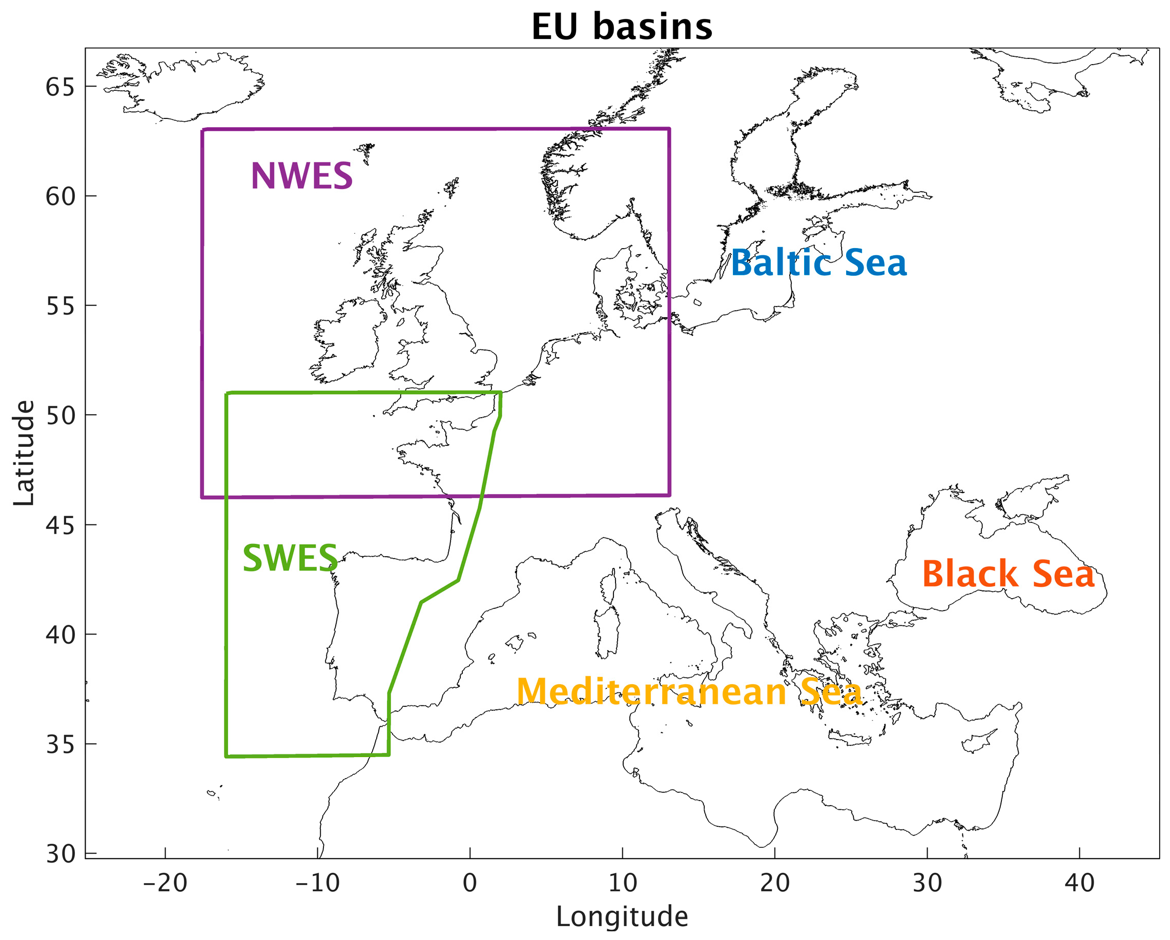
Previous works used the Blue2MF to study plastic distributions with specific Lagrangian models in individual basins: Ichthyop v.3.3 was used in the Mediterranean and Black Seas [3,7,12], and OceanParcels in the Baltic Sea [8]. In this study and within the Blue2MF, the Lagrangian model LTRANS-Zlev (LTRANS hereinafter) [13,14] simulates the trajectories, distribution, and accumulation of macroplastics (plastic particles > 2.5 cm [1]) between 2016 and 2018 for the Baltic Sea, the Black Sea, the Mediterranean Sea, the Atlantic Northwest European Shelf [NWES basin], and the Atlantic Southwest European Shelf [SWES basin] (Figure 1).

The presence of macroplastic litter in marine ecosystems is linked directly with the inputs from land (rivers, beaches, and coastal cities) and from maritime activities (fisheries, transport, sailing, aquaculture, etc.). The LTRANS model incorporates model-estimated macroplastic inputs from land and estimations of maritime (fishing) activities to simulate potential distribution patterns of marine litter for hindcast and forecast time frames, providing valuable insights into the extent and impact of this pervasive form of pollution.

This paper aims to address both the challenges of modelling the spatial distribution and abundances of macroplastic pollution in marine ecosystems with the LTRANS model and the factors that condition the estimation of the model accuracy when model results are compared/validated with the marine litter observations available. This study will provide the basis for future forecast runs to evaluate the impact of policy/management options on marine macroplastic pollution.

2. Materials and Methods

2.1. The Lagrangian Model LTRANS

The experiments carried out in this study for each European basin (Figure 1) use the Lagrangian model LTRANS (v.Zlev) [13,14], and they are based on the assumption that the floating macroplastic particles are transported by surface currents and Stokes drift derived from surface winds [15,16]. All the particles in all the basins, from both land-based and maritime sources, are assumed identical, and no size classes are simulated. Biofouling, fragmentation, sinking, and windage are not included. Once a floating macroplastic particle enters the open sea from its source, it may circulate within the basin, accumulate at the coastline, or escape from the basin by the open boundaries.

To simulate the distribution of plastics at each basin using LTRANS, the following datasets are required as input:

• The sources of macroplastics, which include both land sources and sea sources (maritime). Each macroplastic (or particle) is released at the surface at a specific time and location in each one of the basins. A detailed description is in Section 2.2.
• The 3D marine currents for each marine basin, which are computed with the General Estuarine Transport Model-GETM [17]. GETM is the hydrodynamic model within the JRC Blue2MF. The horizontal resolution of the GETM runs is specific for each basin: 4’ × 2’ for the Baltic Sea, 2’ × 2’ for the Black Sea, 5’ × 5’ for the Mediterranean Sea, and 5’ × 3’ for both the NWES and SWES basins. The atmospheric forcing datasets used as inputs in GETM are from the European Centre for Medium-Range Weather Forecasts (ECMWF-ERA5).
• The Stokes Drift fields also condition the marine macroplastics distributions [15,16]. For the runs in this study, the Stokes Drift fields used are downloaded from the Copernicus site (https://marine.copernicus.eu/). For our marine basins, they all are computed by wave models using the ECWMF-ERA5 surface winds. The Stokes Drift input files have finer resolution than the marine currents in each basin (Table S5), and the LTRANS runs include them averaged in the same horizontal grid as the marine currents. A detailed description is in Section S3.
• The bathymetry file of each marine basin, which is the same one used by the GETM hydrodynamic-model setup to compute the 3D marine currents.

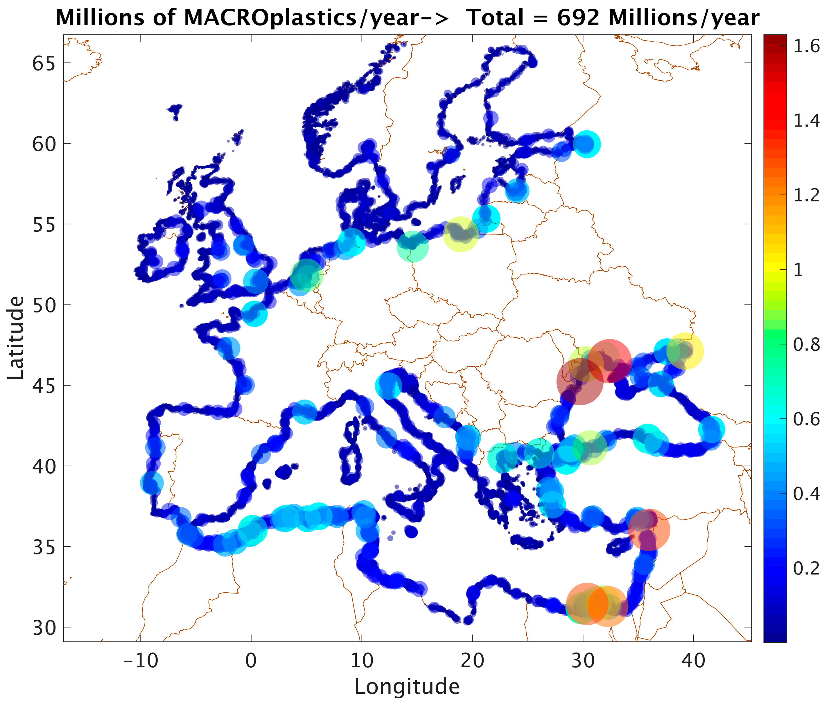
To simulate the trajectories of the macroplastics at the marine surface layer, the released particles are forced by the LTRANS model to remain at the surface by prescribing a vertical upward velocity. The data on the abundances of the macroplastics released in each specific source are available in units of number of macroplastics (or particles) per month per specific source location. Figure 2 shows the sources at the coast (or land sources as described in Section 2.2), with the yearly values of macroplastics per basin in

Table 1. Land-based macroplastics inputs of LTRANS according to the model in [1], per basin, in Millions of macroplastics/year. Some of the basins overlap areas of their geographical domains, and each basin uses all available sources within.

Basin	Land-Based Macroplastic Inputs of LTRANS (Million Macroplastics/Year)
Baltic Sea	64
Black Sea	86
Mediterranean Sea	377
NWES	135
SWES	53

. We have assumed that the monthly release of macroplastics in each source location is distributed homogeneously daily.

The LTRANS results for each released particle (or macroplastic) are the daily position in the basin and the status of the particle. The results are saved in daily averages in model-time. For every day in model time, the status of a macroplastic item can be BEACHED, FLOATING, FLOATING-LOST, or ESCAPED-from-the-basin. The marine-basin geographical domain in the model can have open boundaries connecting with other basins. For example, the Strait of Gibraltar is an open boundary connecting the Mediterranean Sea and the SWES basin (Figure 1). Through those open boundaries, particles in LTRANS can escape. Therefore, they are not included anymore in the results.

The FLOATING-LOST status is due to the length of the runs: because of computer-power constraints, the macroplastics released every day are in a run for 6 months (in model time) after the day of release. For example, the LTRANS results on 1 January 2018, include the information on the particles released from July 2017, but not of others released previously. We have found that a negligible percentage of the macroplastics released had FLOATING-LOST status due to this run duration of 6 months.

2.2. The Sources of Macroplastics as Inputs in LTRANS Runs

For macroplastic pollution, we need to consider in general two main sources: land-based inputs, which are the more important numerically, but also maritime-based. By examining together the land-source and the sea-source estimates of macrolitter described below, we aim to get a more complete picture of the actual load of macroplastic inputs to EU marine regions to force the LTRANS model.

2.2.1. Land-Based Macroplastic Inputs

Following the study presented in [11], we use the macroplastic input estimates provided by the model of [1] updated to include also all non-European countries in the basins (Section S1, [18]). In short, this approach uses floating macrolitter flux data collected in rivers across Europe [19] to calibrate an empirical model relating mismanaged waste generated in the drainage basin to the annual litter loading to the ocean. The mismanaged waste generation was calculated by [1] using a modification of the approach in [20], intersecting data from geographic information system (GIS) layers of population density and drainage basin delimitation. The database covered from small streams to large European rivers, such as the Danube, Vistula, Douro, Rhone, and Tiber. The basin size ranged from 1 to 800,000 km², the population ranged from 1000 to 80 million inhabitants, and the mismanaged waste ranged from 3000 to 6 million tonnes per year [1].

We use the litter estimates from the model in [1], including both European and non-European land sources, as inputs for the LTRANS runs. They are distributed monthly and extrapolated in the model grid. These monthly releases are distributed proportionally to the monthly average surface runoff estimates for each drainage basin considered in the model and its corresponding source location. Monthly average runoff estimates were extracted from the Copernicus Climate Change Service (C3S) dataset [21].

A summary of the results per basin is given in Table 1 and Figure 2. Overall, the yearly estimate is close to 700 million macroplastics per year. This value is consistent with the findings reported in [1] for Europe, where the authors estimated an annual input of 626 million macrolitter items into the ocean (80% confidence interval: 307–925 million), with plastics accounting for approximately 82% of this total.

As shown in Figure 1, some of the basins overlap small areas of their geographical domains: the Baltic Sea and the NWES basin overlap on the Danish Straits, the NWES and SWES basin over the Atlantic Ocean, and the SWES and the Mediterranean Sea in a limited area near the Strait of Gibraltar. We run LTRANS independently for each basin, and with all sources available within its domain. Thus, some sources are used in two basins. The analysis of the LTRANS results in Section 3 is performed for each basin separately.

For the land sources in the LTRANS runs, we also assume:

• The LTRANS domain for the Mediterranean Sea does not include the Marmara Sea. For this reason, and given the direction of the currents at the Dardanelles Strait toward the Aegean Sea, we assume that the total amount of macroplastics released by the sources around the Marmara Sea is entering the Mediterranean Sea by the Strait of Dardanelles.
• Following the same rationale, the macroplastics released in the Azov Sea are entering the Black Sea via the Strait of Kerch.

2.2.2. Maritime-Based Macroplastic Inputs

The total amount of litter from sea-based human activities (fisheries, commercial shipping, sailing, cruises, aquaculture, transport, etc.) is not currently known [22]. Also, it is difficult to identify/distinguish if a plastic litter (e.g., plastic bottles, bags, etc.) found at sea or at the beaches comes directly from land or from maritime activities.

Fisheries-related litter items are, however, more easily identifiable and can account for the majority of the marine-based litter [22,23]. We, thus, assume that fishing ships are responsible for a large fraction of the macroplastics released in the sea.

We have followed two different approaches to estimate the number of fisheries-related items as sources of macroplastics: the first one is using the beach monitoring data from the EU Marine Strategy Framework Directive (MSFD) reported by EU Member States through the European Marine Observation and Data Network (EMODnet) litter-dataset (https://emodnet.ec.europa.eu/en/chemistry, accessed on 1 December 2023). The second one is using an estimated production of litter by each fisherman at annual basis, following the same approach as in [24]. As detailed in Section S2.1 of the Supplementary Materials (providing information on both methodologies), the first approach is likely understimating the total input of fisheries-related items into the marine environment, although both methods provide comparable numbers. Thus, we used the second approach (Section S2.2) based on the number of people involved in the fishing sector [24,25] to calculate the fisheries-related litter estimates to be used in LTRANS as inputs for the different MSFD regions. The resulting values are in

Table 2. Estimates of the total amount of fisheries-related macroplastics using the approach in [24].

Basin	Fisheries-Related Macroplastic Inputs of LTRANS (Million Macroplastics/Year)
Baltic Sea	1.2
Black Sea	4.4
Mediterranean Sea	30.7
North-East Atlantic	9.7

.

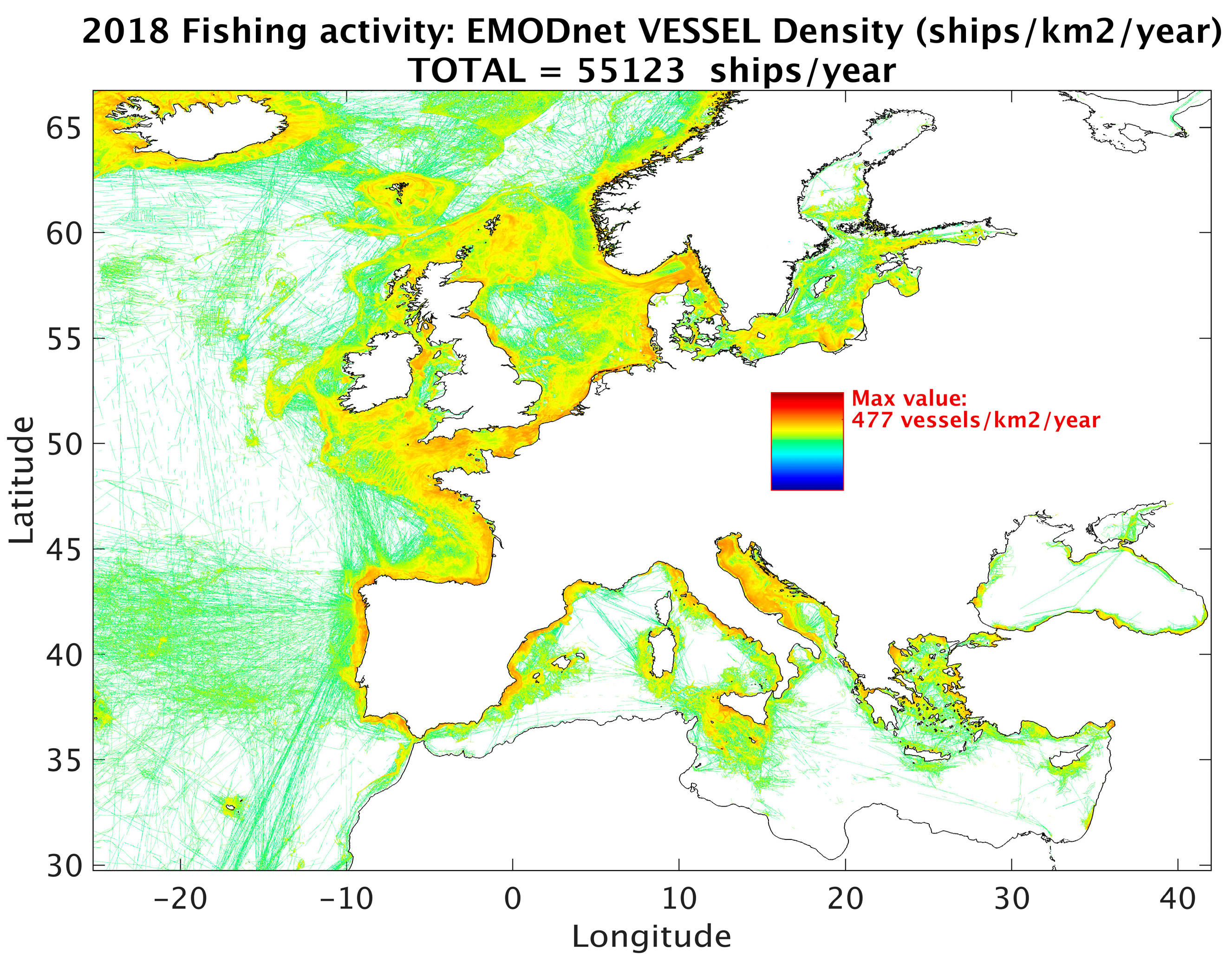
To spatialize the inputs of fisheries-related items due to the heterogeneous distribution of fishing activities, we use the EMODnet monthly data on fishing vessel density derived from AIS (Automatic Identification System) records (see the example for 2018 in Figure 3). It must be noted that only boats larger than 15 m are obliged to install AIS. Henceforth, smaller fishing vessels are not considered in the density data below. We use the EMODnet-vessel-density monthly dataset to calculate the number of fishing ships in each basin, and we distribute the maritime-based macroplastics abundance among them, assuming homogeneous daily release within each month.

2.3. Observations Available to Validate/Compare with the LTRANS Results

2.3.1. Observations of Macroplastics on the BEACHES

The validation of the beached LTRANS results per basin for the hindcast period is carried out by comparing them with the abundances of macroplastics observed on the beaches and provided within the EMODnet litter dataset (https://emodnet.ec.europa.eu/en/chemistry). EMODnet provides access to high-quality marine information supporting research and data related to pollution that are collated, validated, and published using standard protocols and formats [26,27].

The beach litter dataset provided by EMODnet was surveyed by the EU Member States to report to the MSFD. The guidelines for the data collection in [28,29,30] recommend that the reference beaches be surveyed four times a year when possible. The suggested survey periods are as follows: Winter (mid-December–mid-January), Spring (April), Summer (mid-June–mid-July), and Autumn (mid-September–mid-October). They also recommend that the surveyed beaches are exposed to the open sea, have a minimum length of 100 m, and, ideally, are not subject to any other litter collection activities, e.g., cleaning by local authorities. For simplicity, in this study, we will refer to these guidelines as the EMODnet guidelines, although EMODnet does not recommend survey guidelines but aims to collect, homogenize, and distribute the datasets surveyed by the Member States following these guidelines. In the same way, we will refer to the beach litter data collected by the Member States as the EMODnet surveys/sites/observations/data/variables.

The EMODnet variables used for validation include the date and position of the survey-site (or beach), the observed litter items per 100 m, and the description (or category) of the litter. We only use the litter items in the EMODnet file that can be identified as macroplastics: by selecting the corresponding categories or types of litter that correspond to sizes > 2.5 cm. We do not include the categories of litter that may likely come from land being directly deposited on the beach.

2.3.2. Observations of FLOATING Macroplastics at Open-Sea

The observations available for this study for floating macrolitter correspond to the Mediterranean Sea, the Black Sea, and the SWES basin.

For the Mediterranean Sea, observations are coming from the MEDSEALITTER project coordinated by the Istituto Superiore per la Protezione e la Ricerca Ambientale-ISPRA (Rome, Italy). The MEDSEALITTER project is an INTERREG Mediterranean project that benefited from observations by commercial ships and ferries throughout their navigation-transects repeated in the basin. Between 2016 and 2018, the ships and ferries collected 7780 observations of floating litter at different times and locations by visual inspection, following a common systematic monitoring protocol described in detail in [31]. These observations provide extensive standardized information on floating marine litter. When we group the MEDSEALITTER observations within the grid cells of the horizontal grid of the Mediterranean Sea, the ship transects Sicily-Sardinia and Sicily-Tunisia, accumulating the largest number of observations per transect (Figure S4). For simplicity, we will also refer to the grid cells as pixels.

For each MEDSEALITTER observation (or individual floating-item observed) within a specific transect, we have the observation time, position in longitude and latitude, and litter-material information, together with the ship speed, strip width, and sea state at the observation time. According to the information on the litter material, 93% of the observations are floating macroplastics. The MEDSEALITTER variables allow the calculation of the density of floating macroplastics by following the formulation in [32], as described in Section S6 in the Supplementary Materials.

The Black Sea observations utilized in this study were obtained from the EU-UNDP Project “Improving Environmental Monitoring in the Black Sea EMBLAS-II” (https://emblasproject.org/), which pioneered large-scale monitoring of floating marine macrolitter in the region [33,34]. The dataset comprises 302 observations, with 132 collected in 2017 and 170 in 2019, spanning both coastal and offshore areas. The EMBLAS-II project collected data on the date, location, and abundance of floating macrolitter per km² through visual inspections during multiple research cruises in the Black Sea. Notably, plastic items accounted for approximately 96% of the total observed items, as reported in [34]. Further details on the observation locations and characteristics of the collected macrolitter can be found in [33,34].

For the SWES basin, floating-litter densities are available from the CleanAtlantic project coordinated by the Centro Tecnologico del Mar—Fundacion CETMAR (Vigo, Spain). CleanAtlantic is an INTERREG Atlantic Area Programme project that aims at protecting biodiversity and ecosystem services in the Atlantic area by improving capabilities to monitor, prevent, and remove marine macrolitter [35]. The CleanAtlantic partners share/contribute with marine litter observations collected by direct-visual inspections and/or imagery tests with drones, during international oceanographic surveys between 2007 and 2020 in the Atlantic area. A detailed description is provided in https://www.cleanatlantic.eu/results/ (accessed on 26 September 2024). The CleanAtlantic densities used for quantitative comparison with LTRANS are available online at https://www.cleanatlantic.eu/MarineLitterViewer (accessed on 26 September 2025) and derive from direct-visual observations. These densities are grouped within the standardized grid cells of the International Council for the Exploration of the Sea (ICES cells or pixels), with a horizontal resolution of 0.5° in latitude and 1° in longitude. The collecting times of the CleanAtlantic observations are different in each ICES pixel, and they are scattered between 2007 and 2020.

2.4. Comparison of Model Results with the Available Data

2.4.1. Comparison of Model Results with Data on the BEACHES

We examine the model accuracy for beached macroplastic by comparing the LTRANS results with status BEACHED in the simulated period with the abundances of macroplastics provided by the EMODnet litter dataset, for the same dates and locations of the surveys in EMODnet.

For the comparison, we group the number of observed macroplastics by survey site (or beach) for the specific survey day, and we assume that the units are the number of macroplastics per 100 m accumulated since the previous monitoring survey in that site. Thus, the EMODnet data represent a flow of macroplastics accumulated on a beach within a period of time (or number of items per 100 m per time interval during accumulation), which is related to survey periodicities.

Two factors are considered to compare the EMODnet and the LTRANS densities: first, the actual periodicity of the EMODnet surveys on a specific site, and second, the number of LTRANS macroplastics in the EMODnet dates and locations, taking into account the beached time (or time of residence) of the litter in the site and the horizontal model resolution of the basin in each LTRANS run.

To ensure comparability with the LTRANS model results, which simulate particle trajectories over a 6-month period, we examine the survey periodicities in each EMODnet site and only include those with a preceding observation within 6 months. This criterion allows us to minimize temporal discrepancies between the survey data and model outputs. Additionally, we include the initial survey at each EMODnet site in our analysis, assuming that the site was cleaned of macroplastics at least 6 months prior to the first survey. This assumption enables us to establish a baseline for comparison, ensuring that the survey data are as comparable as possible to the LTRANS results.

We compute the number of LTRANS macroplastics beached in the EMODnet sites and dates, assuming that:

• The EMODnet surveys included in the comparison (with survey periodicity lower or equal to 6 months) follow the general guidelines in [29,30,31]. Thus, once the litter items are counted and documented, they are removed from the beach, and no extra cleaning (e.g., by the local authorities) is carried out from that moment to the next EMODnet survey.
• The macroplastics in the EMODnet database have all arrived from the sea, and they were not dropped at the beach by beachgoers or other inland polluters.
• The beached time of the LTRANS macroplastics can vary from EMODnet survey to EMODnet survey and within the range of 1 day to the survey periodicity.

Though conditioned by the horizontal resolutions of the LTRANS runs, the particle positions at each model time step are given by LTRANS in a specific location (latitude and longitude). For each EMODnet location and date of survey, we assume a radius of tolerance to include the LTRANS macroplastics around the location, in agreement with the specific mean horizontal resolution of the basin. We build the vector of LTRANS abundances by grouping those macroplastics depending on the maximum beached time from the EMODnet date backwards to a maximum of 6 months. The units of this vector of LTRANS abundances per beach are macroplastics per 100 m of coastline and per each beached time (in days).

Though we know the EMODnet survey periodicities for each beach, we do not know the specific beached time of the EMODnet macroplastics, which can range from 1 day to the total time from the day of the previous survey, within the range of 1 day to 6 months, depending on the survey. In contrast, as mentioned above, the LTRANS vector includes the beached-time information on the macroplastic abundances. Therefore, we search in the LTRANS abundance vector for the closest fit that would match the EMODnet abundance, which will give us an estimation of the maximum beached time of macroplastics closest to the EMODnet abundances. This is, for an EMODnet survey, LTRANS can estimate the approximate beached time of those macroplastics that have been counted in the EMODnet survey. These LTRANS beached-time estimations allow us to discuss the LTRANS model performance in Section 3.1.

2.4.2. Comparison of Model Results with Data of FLOATING Macroplastics at Open-Sea

For the Mediterranean Sea, to make the MEDSEALITTER observations and the LTRANS results as comparable as possible, we compute the MEDSEALITTER density day maps that group/count the observations within the grid cells/pixels of the 5’ × 5’ horizontal grid used by the LTRANS runs in the Mediterranean Sea (Section S6 of the Supplementary Materials). The number of available MEDSEALITTER observations to compute the densities on a specific day and pixel is variable in the maps, since the observations have been collected at specific times and do not periodically cover the entire day. The units for both MEDSEALITTER and the concurrent LTRANS density day maps are the number of macroplastics/km² in a day on each grid cell.

To evaluate the accuracy of the LTRANS model, we conduct a comparison with the MEDSEALITTER data using a range of temporal and spatial tolerances. Specifically, we apply four different time tolerances (±0, ±1, ±2, and ±3 days) and four horizontal tolerances (±0, ±1, ±2, and ±3 pixels), resulting in 16 unique comparison cases. We calculate the correlations between each MEDSEALITTER day map and the corresponding 16 LTRANS day maps, including the tolerances. By only including the day maps with statistically significant correlations as determined by their p-values, we compute the mean correlation and the mean floating density (or best-fit LTRANS floating density) for each comparison case. By examining the mean correlations and the best-fit LTRANS densities for the 16 cases, we aim to identify the optimal combination of temporal and spatial tolerances that yields the best agreement between the LTRANS model and the MEDSEALITTER observations. This analysis will provide an estimate of the uncertainty associated with the LTRANS floating results, both in terms of timing and spatial location, relative to the MEDSEALITTER data.

For the Black Sea, we follow the same methodology and calculate the EMBLAS density maps to compare with the concurrent LTRANS results.

For the SWES basin, the CleanAtlantic densities available are already aggregating observations scattered between 2007 and 2020 in the ICES grid cells, with no detailed information about the collecting time of individual observations. Therefore, we cannot calculate the corresponding density day maps. For this comparison, we use the LTRANS densities averaged from 2016 to 2018.

3. Results and Discussion

3.1. BEACHED Macroplastics: Comparison with Beach Observations and Estimation of Model Accuracy

3.1.1. Periodicity of the Beach Surveys in EMODnet Dataset

Table 3. Number of EMODnet surveys between 2016 and 2018 with periodicity less or equal to 6 months by basin (i.e., with frequency higher or equal to 2 surveys per year) and their corresponding percentage with respect to the EMODnet surveys available within that period and basin. The SWES basin had available surveys only for 2016.

Basin	Number of EMODnet Surveys with Periodicity ≤ 6 Months	% of EMODnet Surveys Used of Total Available
Baltic Sea	669	91.6%
Black Sea	24	100%
Mediterranean Sea	501	72.9%
NWES	135	99.3%
SWES	111	100%

presents the number of EMODnet surveys utilized in the comparison for each basin, as well as the corresponding percentage of the total number of surveys available for each basin between 2016 and 2018. Notably, the Black Sea has a limited number of surveys, with contributions from only two countries: Bulgaria and Romania.

As mentioned in Section 2.3.1, the guidelines to the Member States for the data collection recommend four surveys per year, with periodicity of 3 months approximately and in specific months. If we plot the histograms of the periodicities of the available surveys in EMODnet by basin and by country from 2016 to 2018 (Figure S2), they show that:

• Most of the beaches in all basins were surveyed approximately every 3 months. Some beaches were surveyed, following closely the guidelines in [29,30,31]. This is the case, for example, of the beaches in Spain in both the Mediterranean Sea and the SWES basin, and the Netherlands and Denmark in the NWES basin.
• Beaches with survey periodicities different from ~3 months are, for example, the Latvian beaches surveyed every 12 months, the Bulgarian beaches surveyed only once, the French beaches in the Mediterranean Sea with periodicity ~1 month, and the Italian beaches, where the main survey periodicities were quite variable and scattered around 4 and 8 months.
• The calendar months in which the surveys were carried out (Figure S2) indicate that, for some beaches, litter data for the Winter season were not collected: for example, the beaches of Sweden, Finland, Estonia, and Denmark. In contrast, the Summer is missing or almost missing for Greece, Croatia, and Cyprus, whereas for Latvia and Romania, data were only collected in the Summer.

We have calculated the EMODnet survey periodicities for each beach, but we do not know the specific beached time of the EMODnet macroplastics, which can range from 1 day to 6 months, depending on the survey. In Section 3.1.2, we use these variable survey periodicities and the LTRANS beached-time estimations to discuss the LTRANS model performance.

3.1.2. Number of BEACHED LTRANS Macroplastics in the EMODnet Dates and Locations

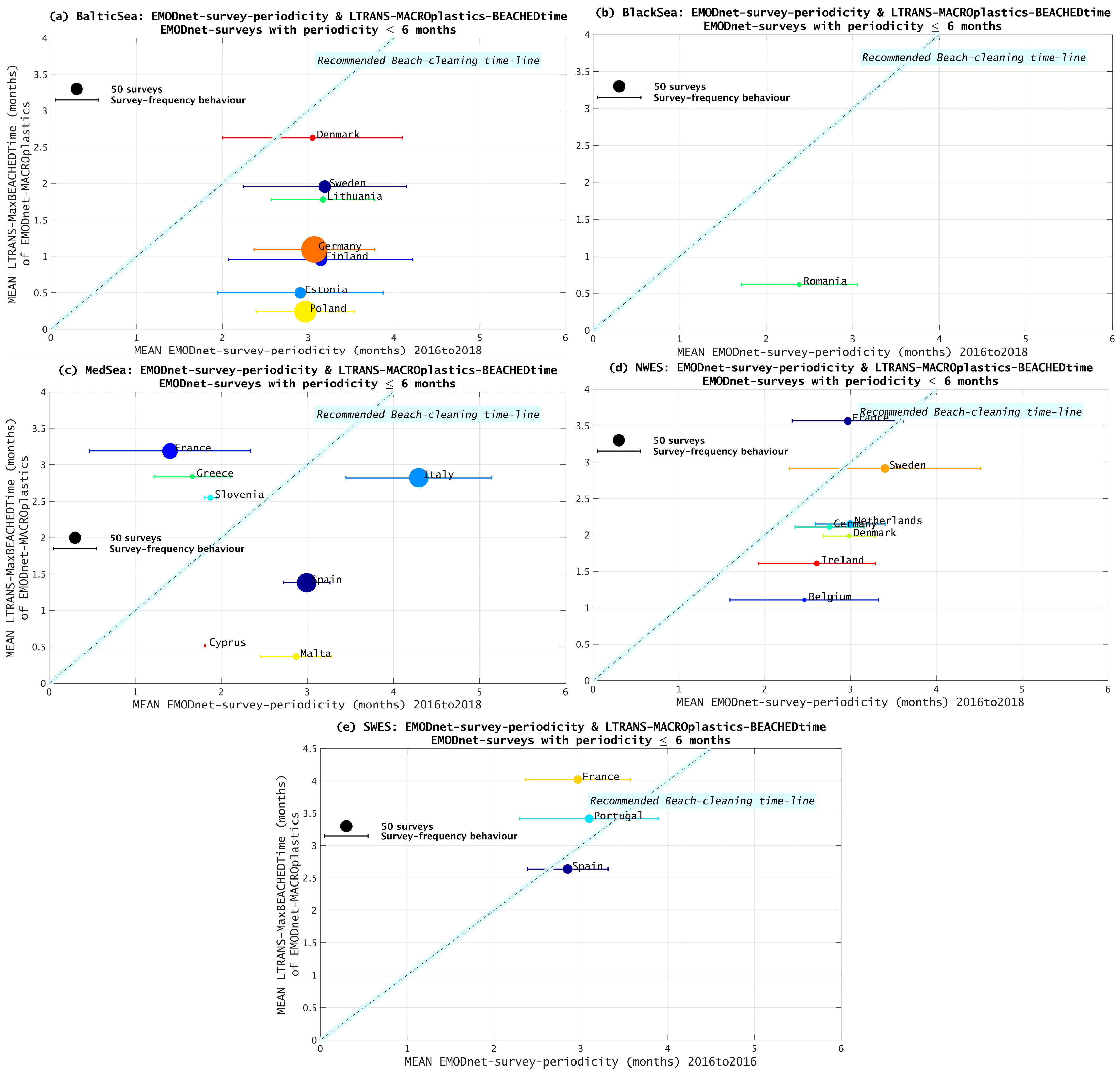
Figure 4 shows the LTRANS beached-times described in Section 2.4.1 (y-axis) plotted against the corresponding EMODnet–survey periodicities (x-axis) for each country in the Baltic Sea (a), the Black Sea (b), the Mediterranean Sea (c), the NWES (d), and the SWES basin (e). The size of the colored circles indicates the number of EMODnet surveys per country, with the standard deviation (STD) of the EMODnet-periodicities in horizontal bars to inform about the range of periodicities used by the EMODnet observers.

The line of “Recommended Beach cleaning timeline” in Figure 4 corresponds to the case in which EMODnet periodicity and LTRANS beached time are equal: if both the EMODnet surveys and the LTRANS model were “perfect”, the colored circles would be on this line. The closer the country circles are to that line, the better LTRANS performed on the corresponding beaches, assuming that circumstances of the EMODnet surveys would have been optimal.

Ideally, if the EMODnet surveys and the LTRANS results were both “perfect” and following the EMODnet guidelines, the EMODnet periodicities and the LTRANS beached times would be equal to 3 months in Figure 4. In reality, we may expect that if LTRANS is producing reasonable results, the LTRANS beached times are no longer than the EMODnet periodicities. If the LTRANS beached times are longer than the EMODnet survey periodicity, it could mean the following:

• LTRANS would need more run-time to accumulate the observed EMODnet abundances.
• LTRANS input sources would not be releasing enough particles in the basin; it would indicate the lack of some sources of litter pollution in the model inputs.
• EMODnet abundances are too large because some litter items do not have a marine-origin. This is, some of the accounted EMODnet macroplastics included may have been produced elsewhere inland and accumulated directly from land to the beach.
• EMODnet abundances are too large because of the fragmentation of macroplastics into smaller pieces. Fragmentation and macroplastic sizes are not included in LTRANS.

Among the countries in the five plots of Figure 4 that have the LTRANS beached time longer than the EMODnet survey periodicity, we may distinguish two different cases. First, Greece and Slovenia in Figure 4c have few EMODnet observations, as also seen in Figure S2a. Second, France in Figure 4c–e, which has very large EMODnet macroplastic abundances in specific locations, as will be discussed later in this section.

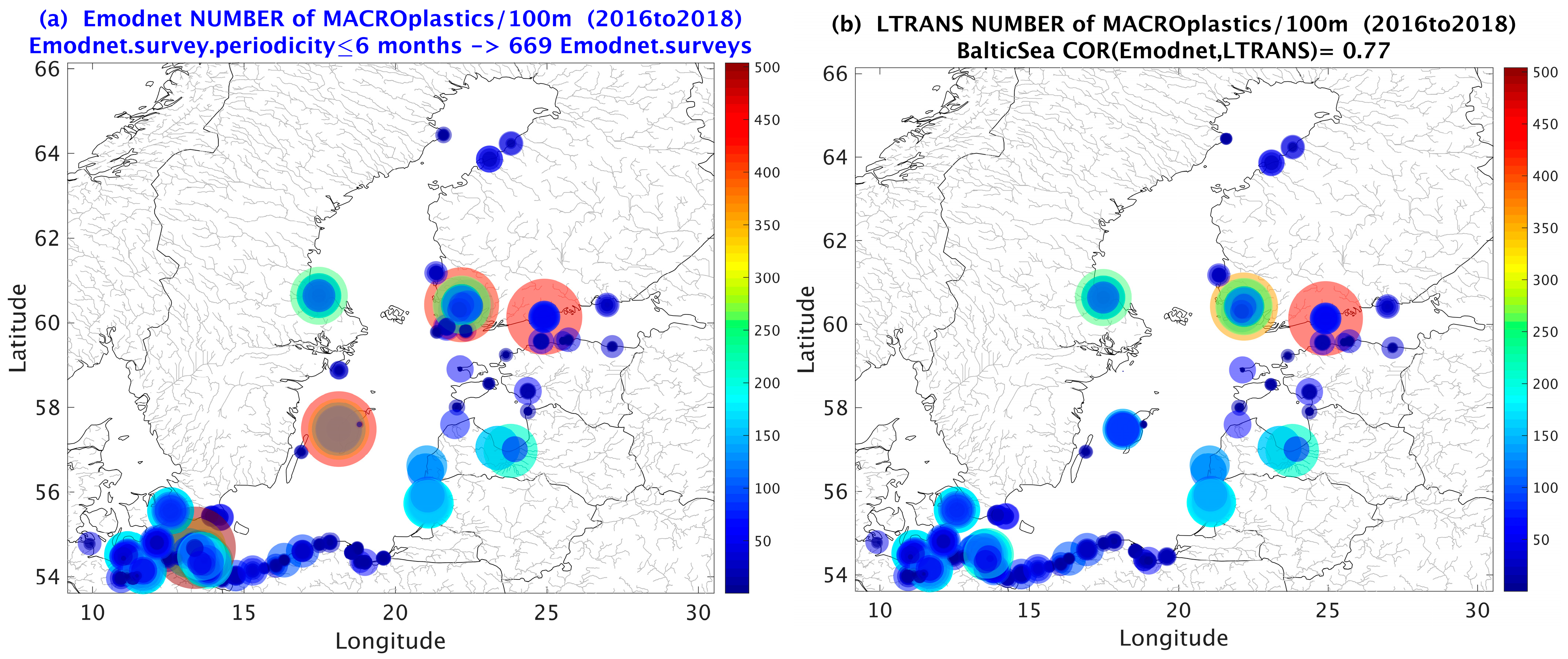
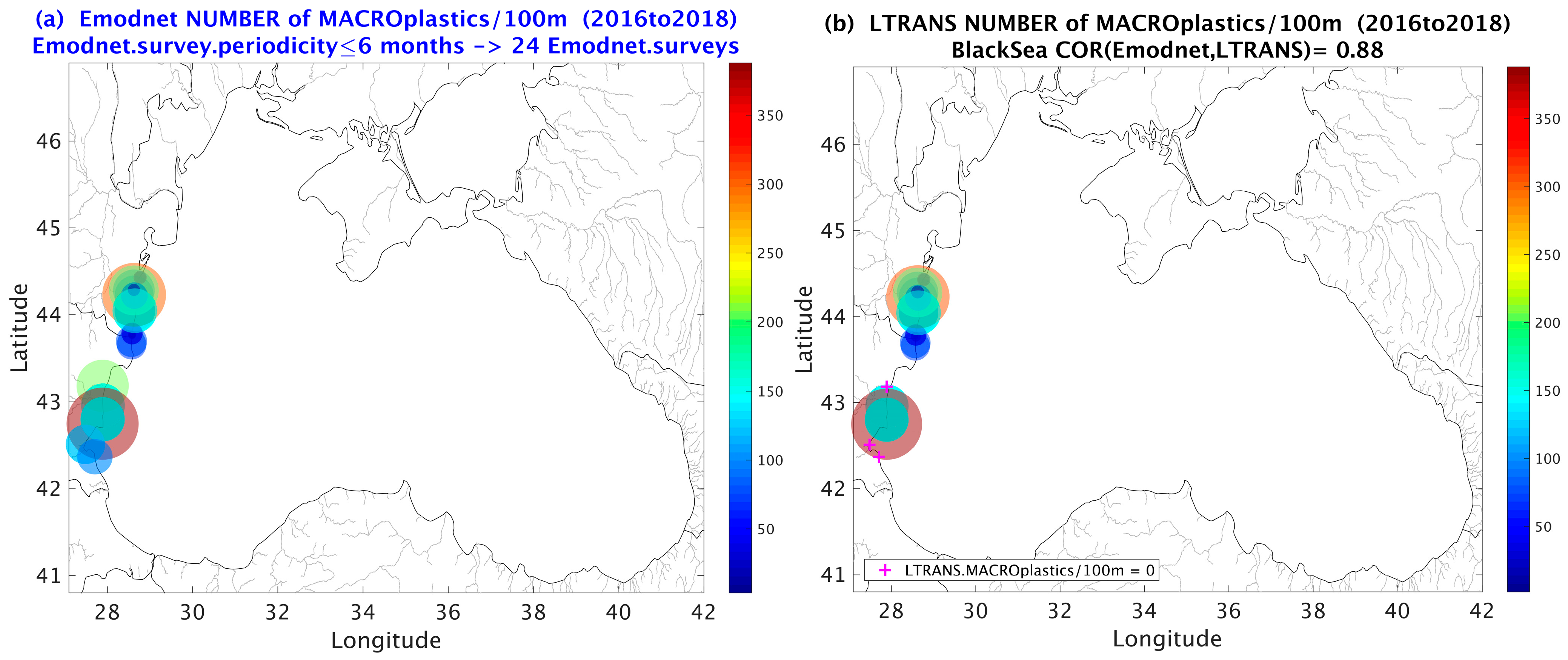
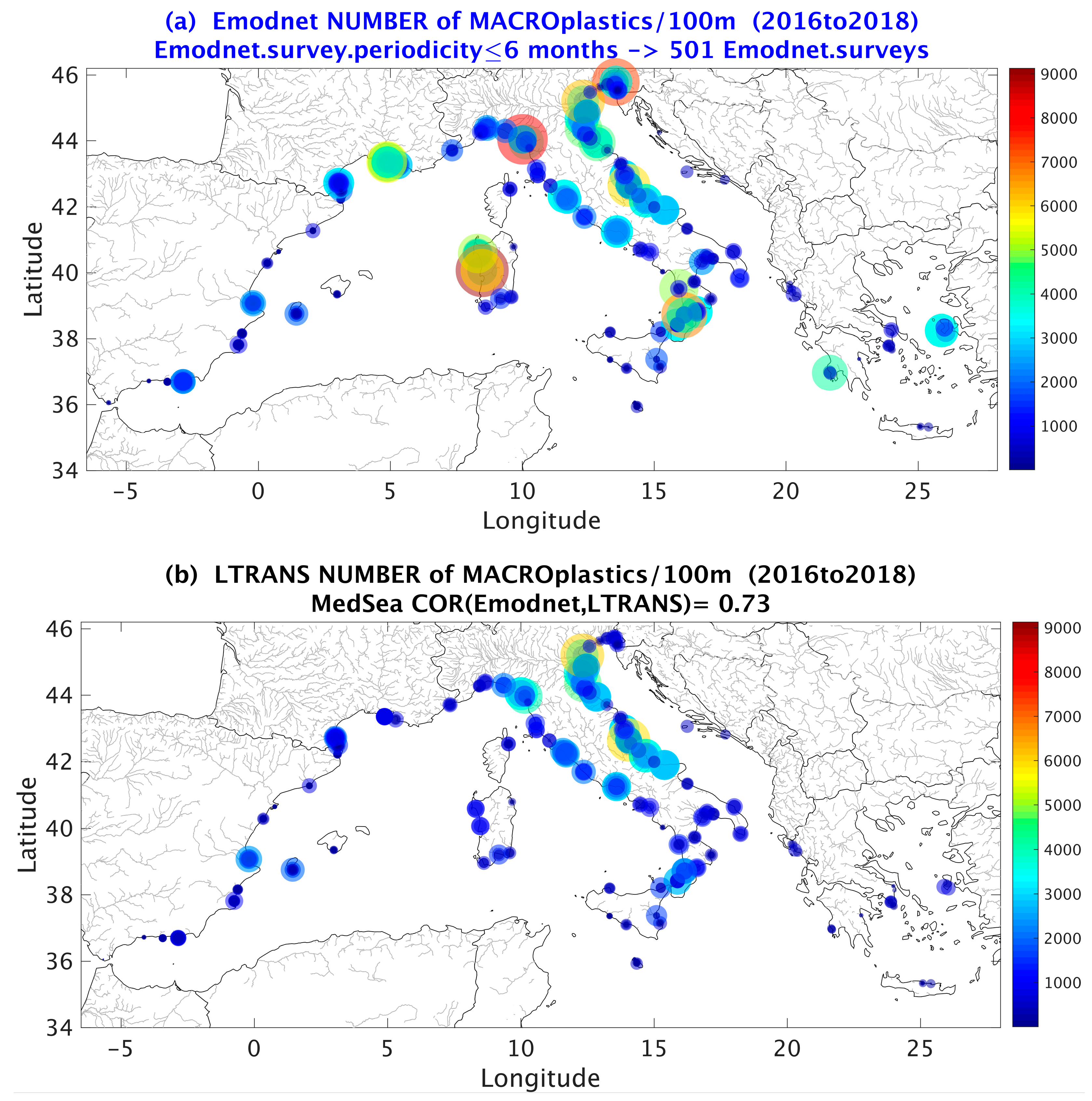
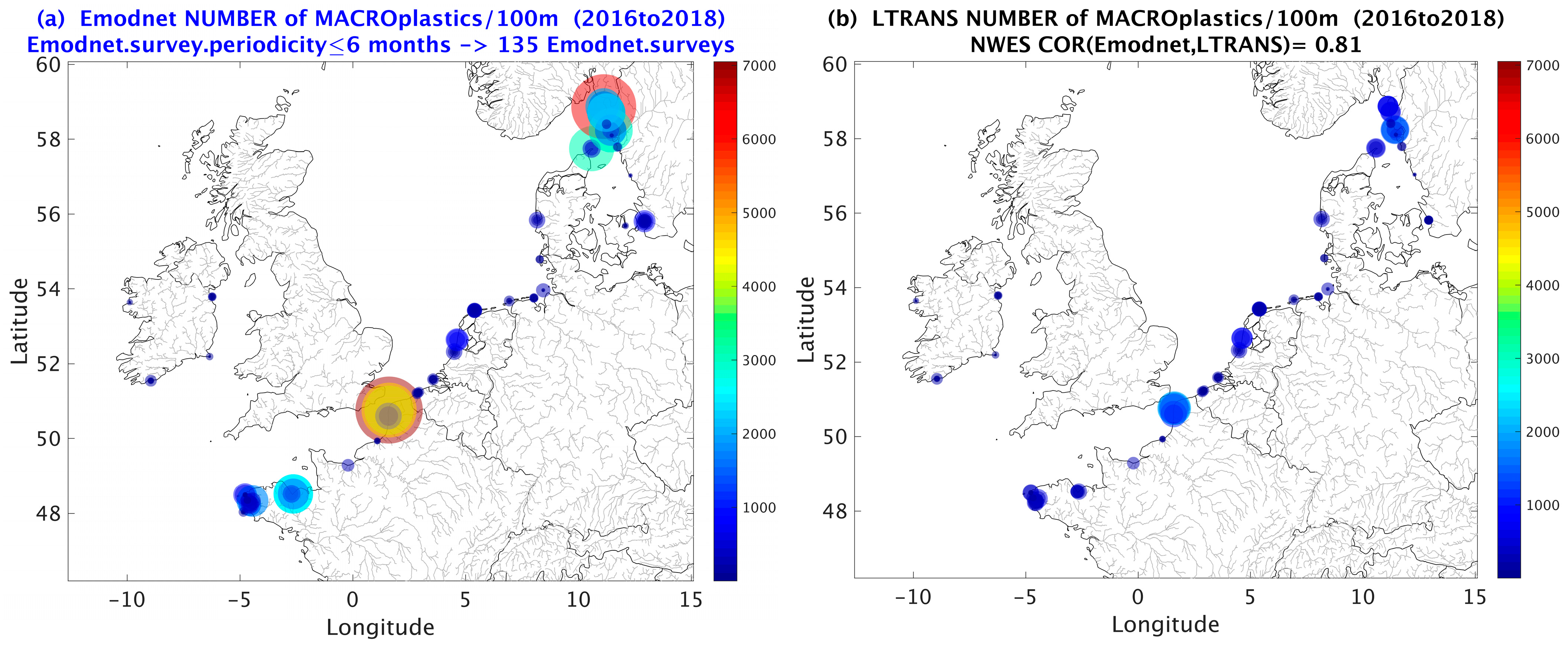
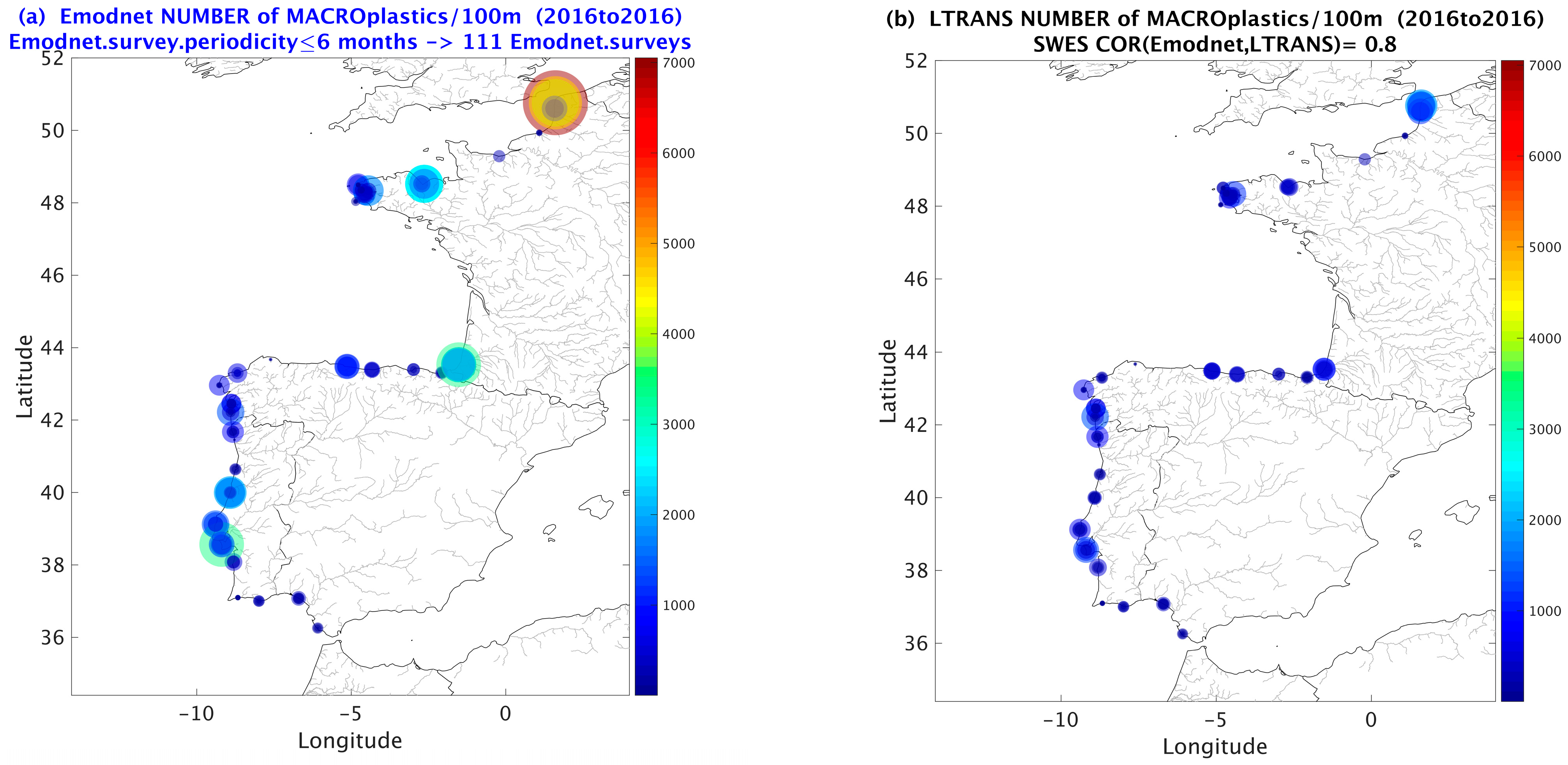
Figure 5, Figure 6, Figure 7, Figure 8 and Figure 9 show the maps with the (a) individual EMODnet abundances per 100 m and (b) the LTRANS predictions, both used in Figure 4. For all of the EU basins, most of the LTRANS abundances in Figure 5, Figure 6, Figure 7, Figure 8 and Figure 9 are similar or lower than those observed by EMODnet. The larger differences between EMODnet and LTRANS values are mainly located close to ports, river mouths, and coastal lagoons. We can see examples in some locations of the German coast and the Gotland Island for the Baltic Sea (Figure 5), close to Marseille and the Rhone mouth, Sardinia, Trieste and the port of La Spezia (Italy) in the Mediterranean Sea (Figure 7), and close to Calais, Biarritz, and Lisbon in the SWES basin (Figure 9). The LTRANS results agree well in general for the Black Sea, though few EMODnet surveys are available. However, in some locations of the Bulgarian coast, EMODnet macroplastics were observed, but LTRANS predicts zero abundances (Figure 6).

Table 4. Correlations between the EMODnet abundances and the LTRANS estimations, minima, and maxima of the correlations within each basin, and the corresponding horizontal resolution.

Basin	EMODnet and LTRANS CORRELATION	EMODnet and LTRANS CORRELATION [Min Values, MAX Values]	Horizontal Resolution km × km (Minute of Longitude × Minute of Latitude)
Baltic Sea	0.77 [1 0.88]	0.52 (Germany), 0.99 (Estonia)	3 to 4.4 km (4’ × 2’)
Black Sea	0.88	0.77 (Bulgaria), 0.99 (Romania)	2.5 to 3.7 km (2’ × 2’)
Mediterranean Sea	0.73 [2 0.74]	0.51 (Greece), 0.99 (Malta)	6.5 to 9.3 km (5’ × 5’)
NWES	0.81	0.71 (Sweden), 0.99 (Netherlands)	4 to 6.1 km (5’ × 3’)
SWES	0.8	0.71 (Portugal), 0.87 (Spain)	5.6 to 7.2 km (5’ × 3’)

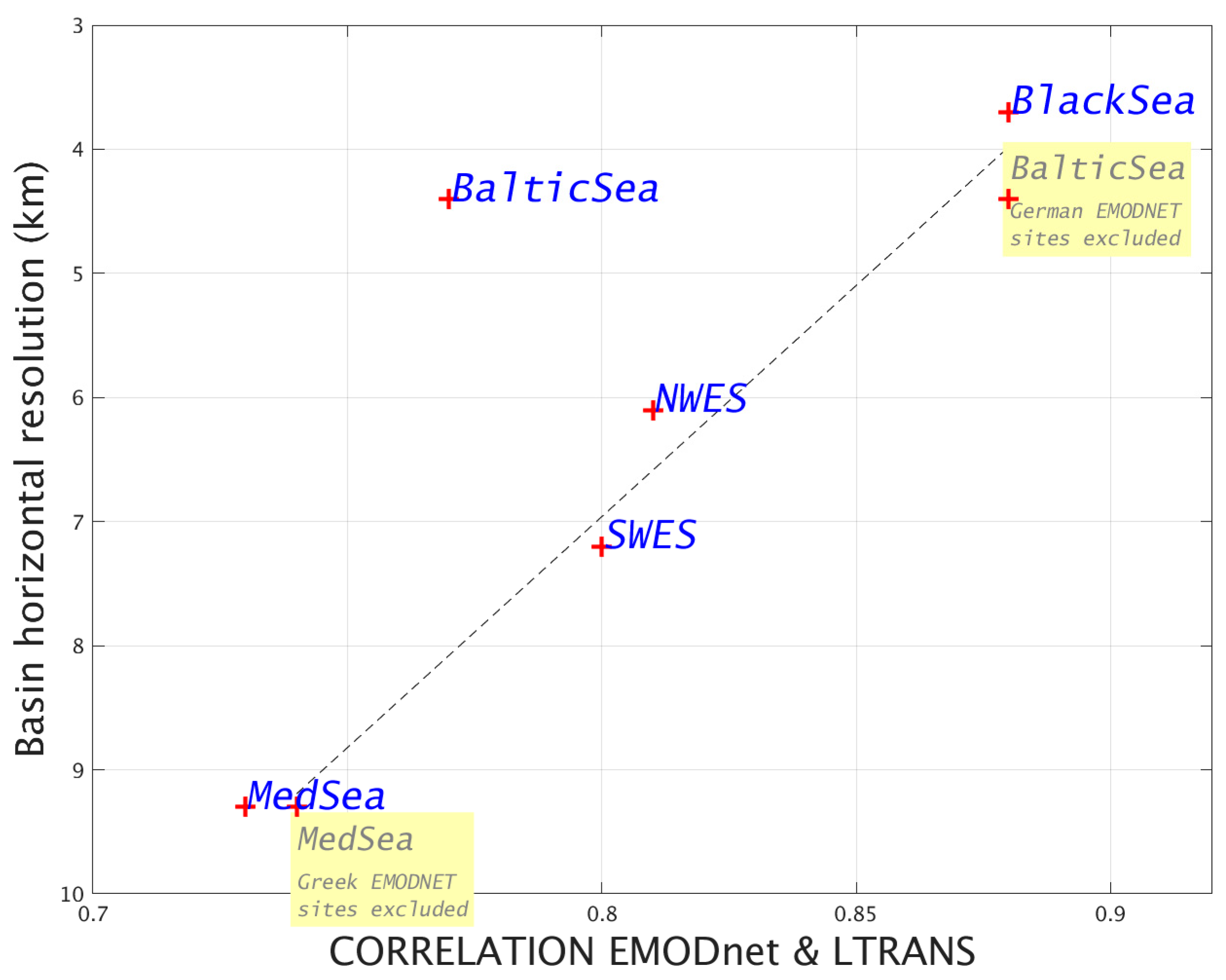
¹ Correlation for the Baltic Sea if the German EMODnet sites are not included. ² Correlation for the Mediterranean Sea if the Greek EMODnet sites are not included.

summarizes the correlations obtained between the EMODnet abundances and the LTRANS predictions, and the corresponding horizontal resolution per basin. The correlations (Pearson correlation) in the EU basins range from 0.73 for the Mediterranean Sea to 0.88 for the Black Sea. All the correlations are statistically significant and with p-value ≤ 2.2 × 10⁻⁶. The p-value = 2.2 × 10⁻⁶ corresponds to the Black Sea.

As shown in Table 4, we find that the lowest correlations by country correspond to Greece (0.51) and Germany (0.52).

For Germany, the larger discrepancies between LTRANS and EMODnet are located in the coast of the Island of Rugen. In Figure 5a, several red circles overlapped in that area, with large values of macroplastic abundances. Ref. [36] studied the macrolitter accumulation in several sites of that island and found that the macrolitter abundance per 100 m was greater than the abundances found in other studies at beaches along the Baltic Sea coast. They also found that macrolitter items were predominantly composed of plastic (83%), and that the impact of wind and water currents, as well as recreational activities, was detectable on the macrolitter accumulation. According to [36], the touristic gradient seemed to have a higher impact on beaches on Rugen, regarding the number of items registered and the relevance of public littering items. Our input estimates might be underestimating the impact of touristic activities in this area, explaining the lower simulated beach litter in the region.

We have not found a specific bibliography about the Greek areas in Figure 7 that shows discrepancies between LTRANS and EMODnet abundances. The Mediterranean Sea is a hot spot for plastic pollution due to its semi-enclosed nature and heavily populated coastal areas, hosting a series of intensive activities such as tourism, fishing, shipping, and industry [6]. For the Greek areas, we might be missing the contribution of some of these litter-producing activities as model inputs, or the EMODnet surveys might include macroplastics accumulated directly from land/beachgoers. Another factor that might help to explain the lower correlation here is the rugged nature of the coast and the relatively low resolution of the ocean model, which does not allow to resolve very local processes.

Therefore, we assume that LTRANS may not predict all the EMODnet macroplastics in those locations in Germany and Greece due to the potential origin in land of a fraction of the observed litter and the inherent limitations of the oceanic model used. If we exclude the German and Greek EMODnet sites, the correlation becomes 0.88 for the Baltic Sea and 0.74 for the Mediterranean Sea (Table 4).

Finally, the horizontal resolution of the LTRANS runs for each basin also conditions the accuracy of the LTRANS predictions. Figure 10 shows the correlations of EMODnet and LTRANS of Table 4 plotted with the corresponding maximum (and therefore less favorable) value of the horizontal resolutions for each basin. The y-axis direction is reverse in the plot, with the coarser resolutions at the bottom and the finer resolutions at the top. If we exclude the German and Greek EMODnet sites from that calculation, the distribution of the points in Figure 10 is almost linear. The dashed line shows the linear fit.

Though it may seem a minor result, it gives robustness to our validation methodology and results, as they are able to confirm quantitatively that the resolution of each basin may condition the final correlation of the EMODnet observations and LTRANS predictions, and, thus, the accuracy of the LTRANS results.

3.2. FLOATING Macroplastics: Comparison with Floating Macroplastic Observations and Estimation of Model Accuracy

3.2.1. Mediterranean Sea: Comparison with MEDSEALITTER Observations

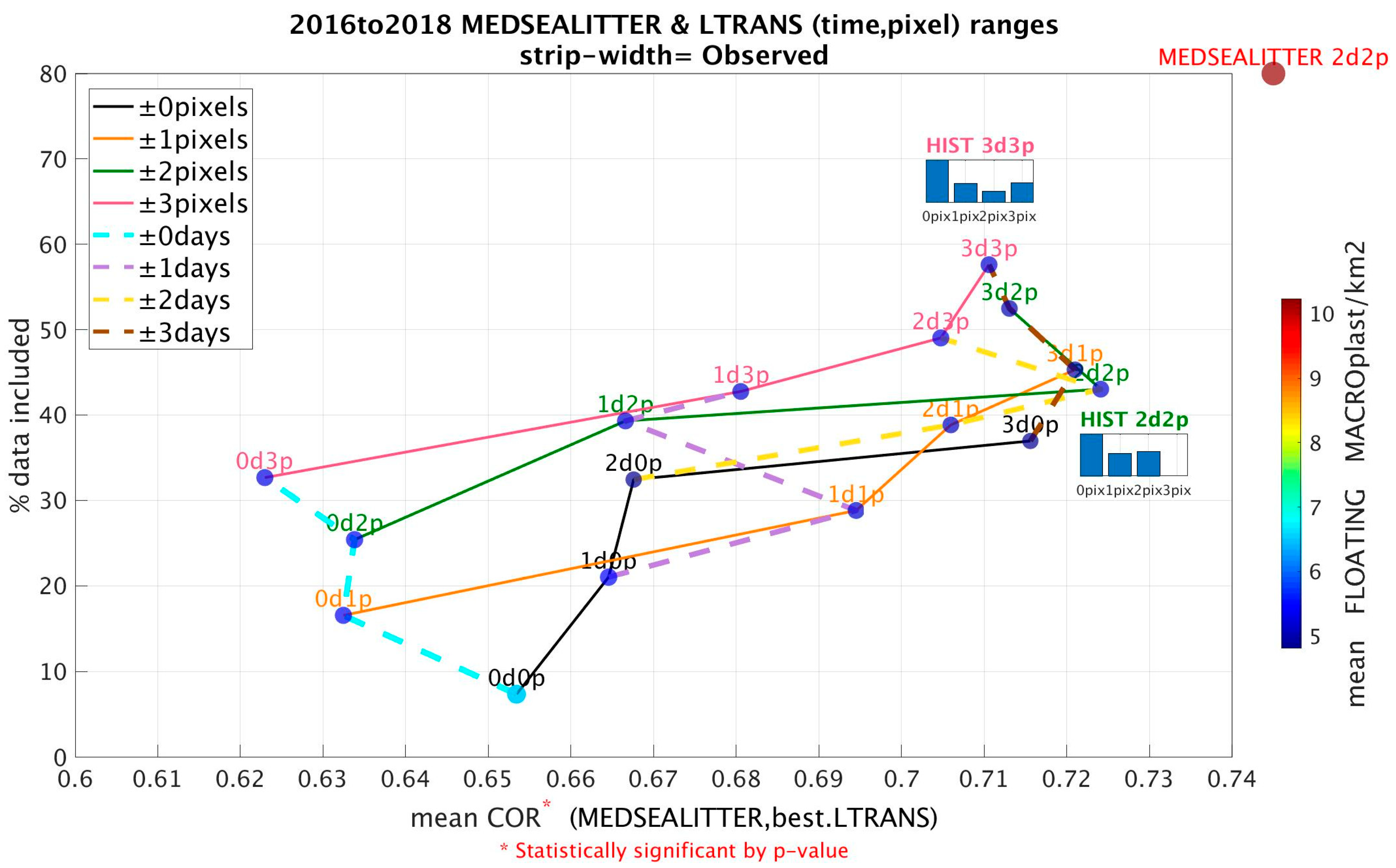
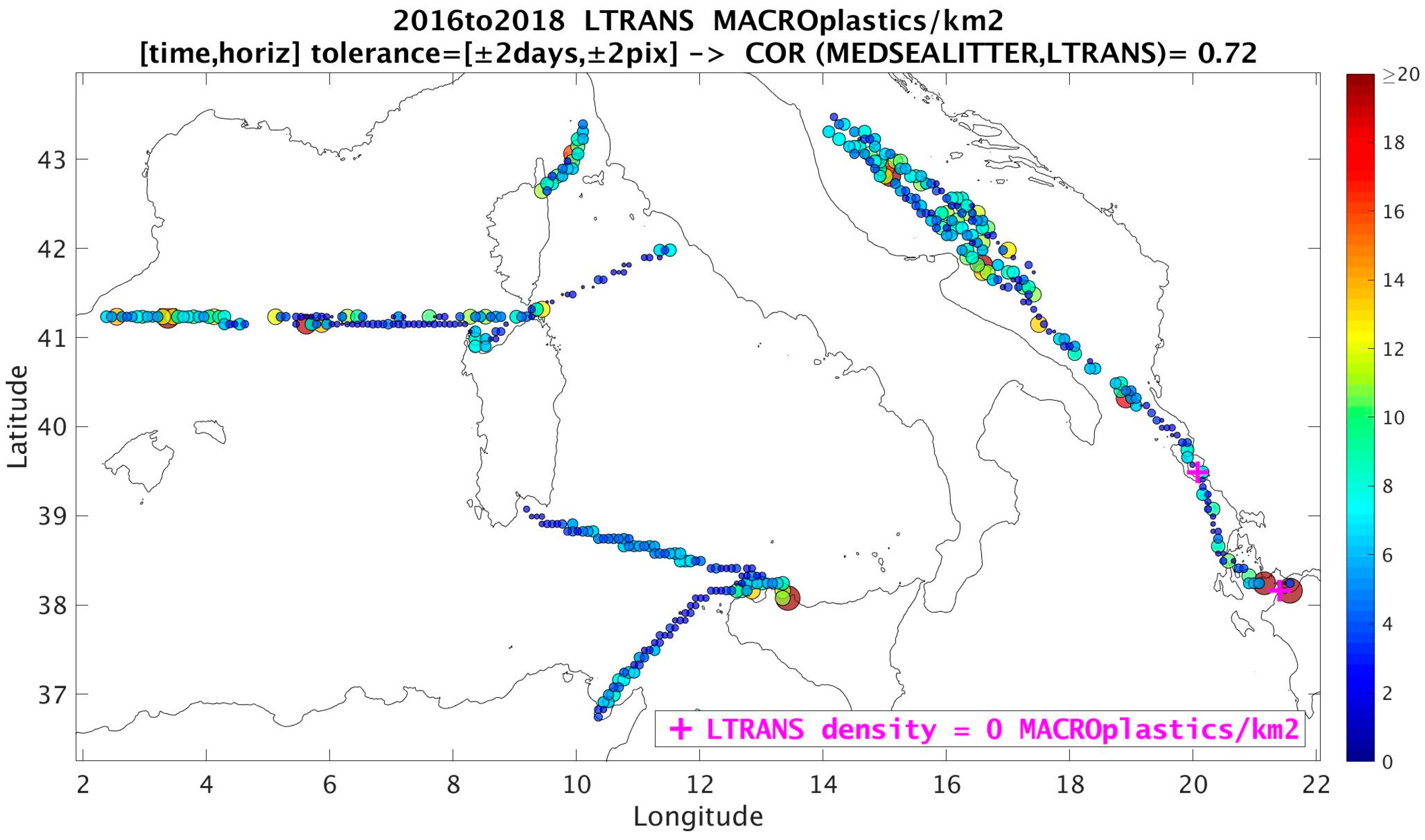
Figure 11 displays the mean correlations between MEDSEALITTER and LTRANS floating densities, considering various time and horizontal tolerances, with respect to the percentages of observations included in the calculations. The percentages of observations result from only including the day maps with statistically significant correlations as determined by their p-values for each comparison case (as described in Section 2.4.2). The analysis examines time tolerances of ±0, ±1, ±2, and ±3 days, as well as horizontal tolerances of ±0, ±1, ±2, and ±3 pixels in the LTRANS day maps. For instance, when comparing MEDSEALITTER and LTRANS at exact day and pixel locations (i.e., tolerances of ±0 days and ±0 pixels, referred to as comparison case 0d0p), the correlation is 0.65, but this is based on less than 10% of the observations (Figure 11). If we examine the cases 0d1p, 0d2p, and 0d3p (they have ±0 days of tolerance or same day, with horizontal tolerances of ±1, ±2, and ±3 pixels, respectively), more observations are included, but we obtain a smaller correlation between MEDSEALITTER and LTRANS. In contrast, if we explore the same pixel locations with time tolerance ±1, ±2, and ±3 days (these are cases 1d0p, 2d0p, and 3d0p in Figure 11), the correlation between MEDSEALITTER and LTRANS progressively increases and reaches 0.72 in the case 3d0p, with almost 40% of the observations included in the comparison.

The comparison case with maximum correlation is 2d2p (for tolerances ±2 days and ±2 pixels), with a mean correlation of 0.724 and 43% of the data included from 2016 to 2018, which are close to the values of case 3d0p in Figure 11.

We obtain that the mean density derived from MEDSEALITTER and that of LTRANS (or best-fit LTRANS) are in the same order, being for MEDSEALITTER ~10 floating macroplastics/km² (red circle on the top right corner of Figure 11) and 6.5–7 for LTRANS (Figure 11). If we use all calendar days within the three years of results of LTRANS, the overall mean LTRANS density is 7 ± 7.5 floating macroplastics/km² (Figure S7).

We have also included in Figure 11 two histograms indicating the horizontal tolerance resulting from the best-fit calculations of LTRANS for the comparison cases 2d2p and 3d3p. For example, for case 3d3p (with time tolerance ±3 days and horizontal tolerance is ±3 pixels), most of the LTRANS day maps with best fit with MEDSEALITTER include pixels (i.e., densities) of LTRANS in the same position (or 0pix in the histograms of Figure 11) as the MEDSEALITTER observation. The same result is seen for the case 2d2p. This is also the case for most of the 16 comparison cases. In contrast, if similar histograms are plotted for the time tolerance, no specific day in the tolerance range of [±0, ±1, ±2, ±3] days is detected as the most common in the best-fit calculations. These results may indicate the following:

• The spatial accuracy of the LTRANS results may be better than the time accuracy.
• The correlation values between MEDSEALITTER and LTRANS densities indicate a time inaccuracy of ±2 days for LTRANS results.

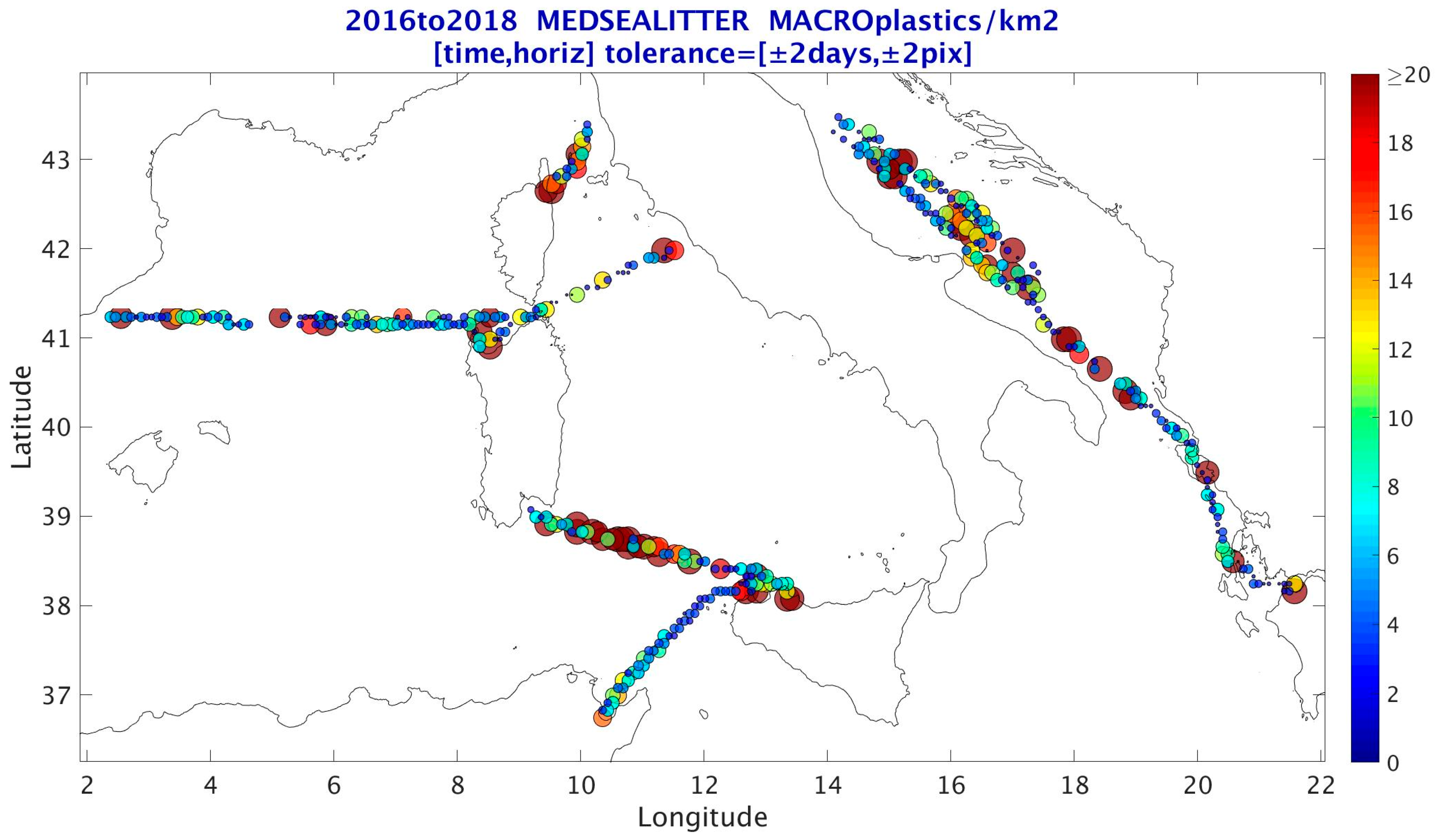
For the 2d2p comparison case, Figure 12 shows the geographical distribution of the MEDSEALITTER densities time averaged for the 3 years, with a large variability in the values even in close pixels over the track of the same transects. It is likely because the time-coordinate of the densities, which depends on the MEDSEALITTER observation time, is distributed irregularly within 2016 to 2018 and reflects different accumulations of macroplastics at different moments. The corresponding LTRANS densities are lower in general than the MEDSEALITTER ones (Figure 13), with an overall mean correlation of 0.72.

The results indicate that the main factors that may condition the comparison between LTRANS results and observations of floating macroplastics, and, therefore, the estimation of the model accuracy, are the following. First, the intrinsic characteristics of floating marine litter data collection at sea, which depend on the ships’ availability, imply that we will have observations only at specific/scattered locations at sea (Figure S4), and with time coordinates unevenly distributed in the time range of the study. MEDSEALITTER collected most of the observations during the summertime of the three years studied, and year 2018 accumulates the largest number of observations (Figure S5).

Another factor is the assumption by LTRANS on the timing of release of the particles in the runs. As mentioned in Section 2.1, the LTRANS inputs on the abundances of the macroplastics released in each specific source are available in units of number of macroplastics (or particles) per month per specific source location. For each source, we have assumed a homogenous daily release of macroplastics within the month. This assumption may introduce partial inaccuracy in the time coordinate for LTRANS floating accumulations when compared with MEDSEALITTER.

To explore further if other factors/circumstances may condition the accuracy in the comparison between LTRANS and MEDSEALITTER densities, we have examined for the case 2d2p the relationship between the MEDSEALITTER-LTRANS correlations with the number of MEDSEALITTER observations included in the calculations, and the potential connection between the MEDSEALITTER-LTRANS correlations with the predicted variability of LTRANS densities. These are the results:

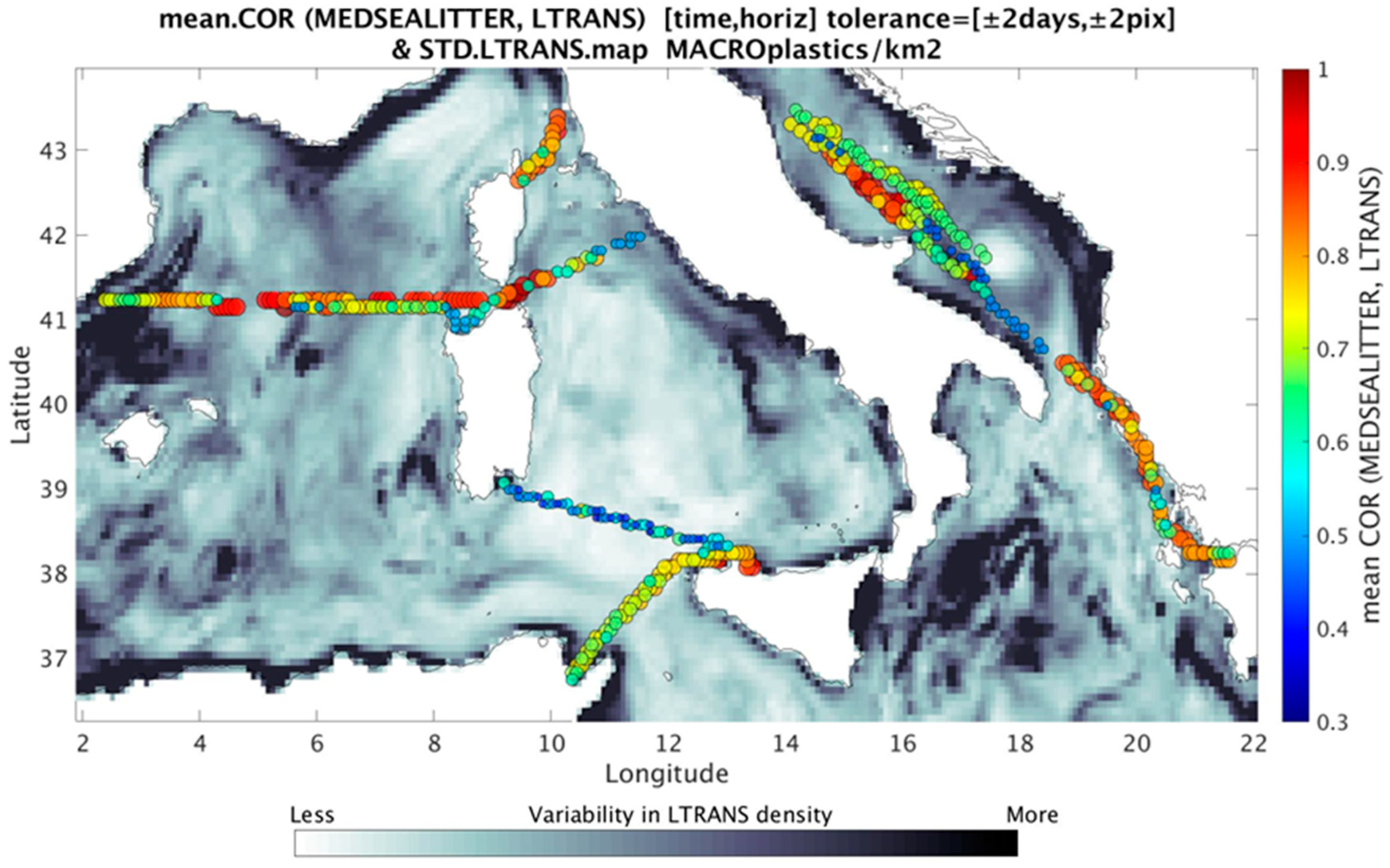
• When we group/count the number of MEDSEALITTER observations according to the corresponding correlations with LTRANS, the histogram shows the maximum in correlation 0.7–0.8 with a Gaussian-like shape, except for a secondary peak in correlation 0.4–0.5 (Figure S8). The corresponding observations of that peak are mostly accumulated in the transect between Sicily and Sardinia (Figure 14), which is precisely one of the transects with many MEDSEALITTER observations available (Figure S4). It is, as well, the transect where the strip-width is mostly 50 m, instead of the more usual 100 m (Figure S9). If the strip-widths were 100 m, most densities of that transect (dark-red circles in Figure 12) would decrease and get closer values to LTRANS values (according to Equation S1 in Section S6 of the Supplementary Materials). The other transect from Sicily, going to/from Tunisia, also accumulates many observations (Figure S4) but has strip-widths of 100 m (Figure S9) and correlations larger than 0.6 (Figure 14).
• The geographical distribution of the MEDSEALITTER-LTRANS correlations overlaps the variability-map of the densities predicted by LTRANS in Figure 14. The variability is estimated with the standard deviation of the 3 years of LTRANS results, as a measure of the spread of the potential density values. We want to explore if the low values of MEDSEALITTER-LTRANS correlations may correspond to areas with large, predicted variability in the LTRANS density, meaning that the MEDSEALITTER observations at specific times may not be representative of the densities than LTRANS can calculate, if the number of macroplastics varies a lot with time in that area. In Figure 14, the low MEDSEALITTER-LTRANS correlations (dark-blue circles) are mostly distributed in areas with local higher variability estimated by LTRANS (darker-grey areas), mostly close to the coast. The exception is precisely the transects between Sicily and Sardinia, also mentioned in the previous paragraph.

Finally, regarding the sea-state information available for each MEDSEALITTER observation, the heavier sea-state encountered corresponded to value 3 in the Beaufort scale [31], and this sea state occurred during 0.007% of the observations. Excluding them has no impact on the results.

3.2.2. Black Sea: Comparison with EMBLAS Observations

When comparing the EMBLAS and LTRANS density maps, we find that the correlation is significant for two comparison cases: 2d2p, with a correlation of 0.29 (p-value = 0.0007), and 3d3p, with a correlation of 0.35 (p-value = 0.00004).

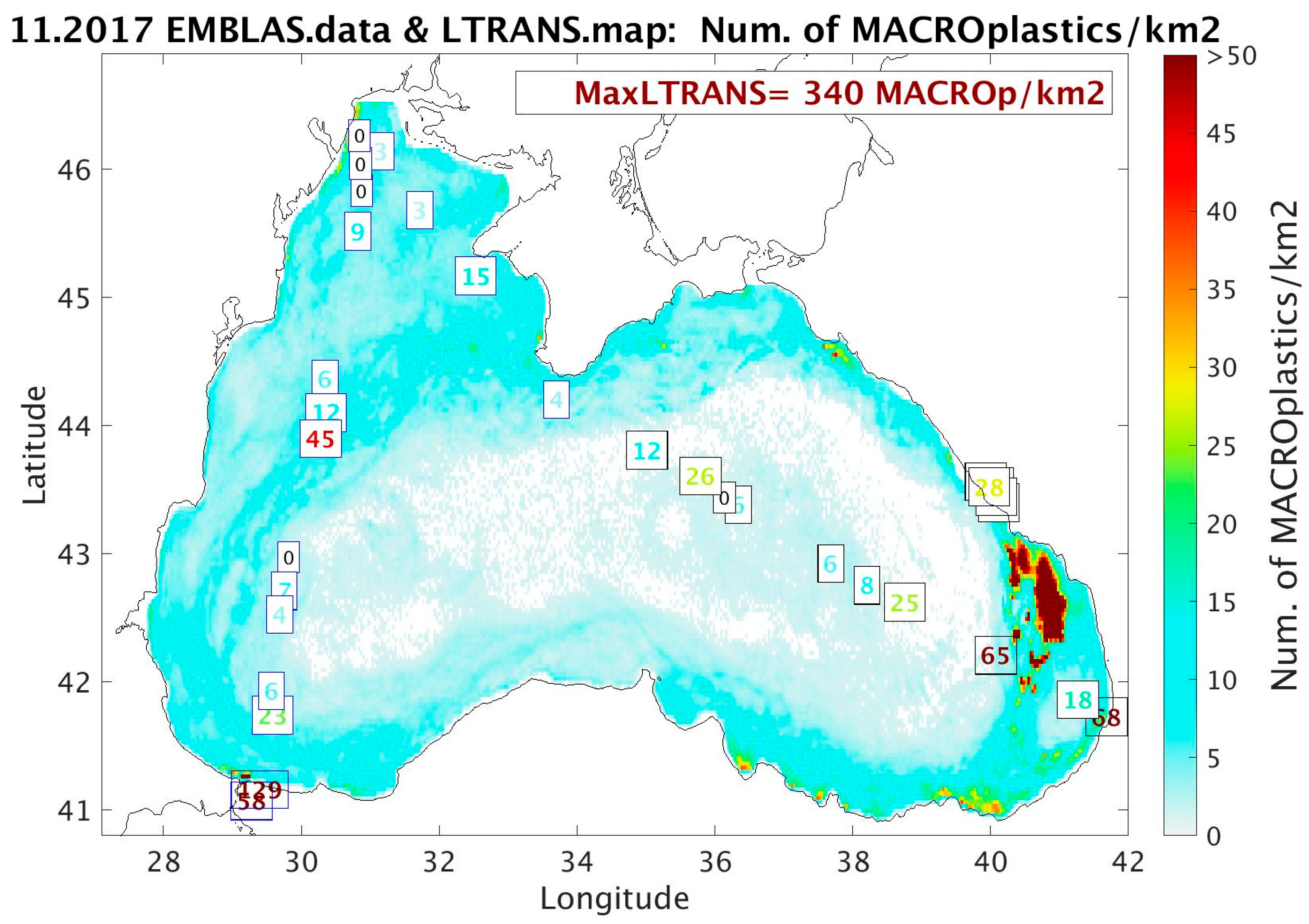
Notably, the majority of the 132 EMBLAS observations available for this study are concentrated in November 2017. Figure 15 illustrates the EMBLAS values at their corresponding monitoring locations, alongside the average LTRANS density map for that month. Although the EMBLAS observations are scattered horizontally and temporally throughout November 2017, both datasets show a consistent pattern of higher floating macroplastic accumulations in the Eastern Black Sea and lower accumulations in the western part.

This spatial gradient is also evident in the monthly averages of the 3-year LTRANS hindcast in the Black Sea (Figure S3), which reveals a persistent pattern of higher litter densities in the southeast, beyond local coastal accumulations. Furthermore, the plots show litter accumulations during the summer months in the NW shelf-break zone, consistent with the model results reported in [3]. The agreement between LTRANS and EMBLAS is particularly notable in the Eastern Black Sea, where both datasets indicate relatively high densities in offshore areas, away from coastal waters. This result is consistent with [34], which suggests a long-term accumulation of floating items in the eastern basin, potentially forming a “garbage patch”, where litter items are trapped, with elevated densities compared to surrounding areas (Figure 15 and Figure S3).

In terms of mean densities, the LTRANS estimates for the 3d3p case are 30 ± 40 macroplastics/km². In contrast, Ref. [34] reports EMBLAS densities of 82 ± 89 items/km², with 95.8% of these items being plastic. The LTRANS abundances are lower than the observed values, which may be attributed to the limited number of observations available for the Black Sea compared to the Mediterranean Sea. Additionally, the same factors discussed in Section 3.2.1, which affected the comparison between LTRANS results and MEDSEALITTER observations, also influence the model’s accuracy in this basin.

3.2.3. SWES Basin: Comparison with CleanAtlantic Data

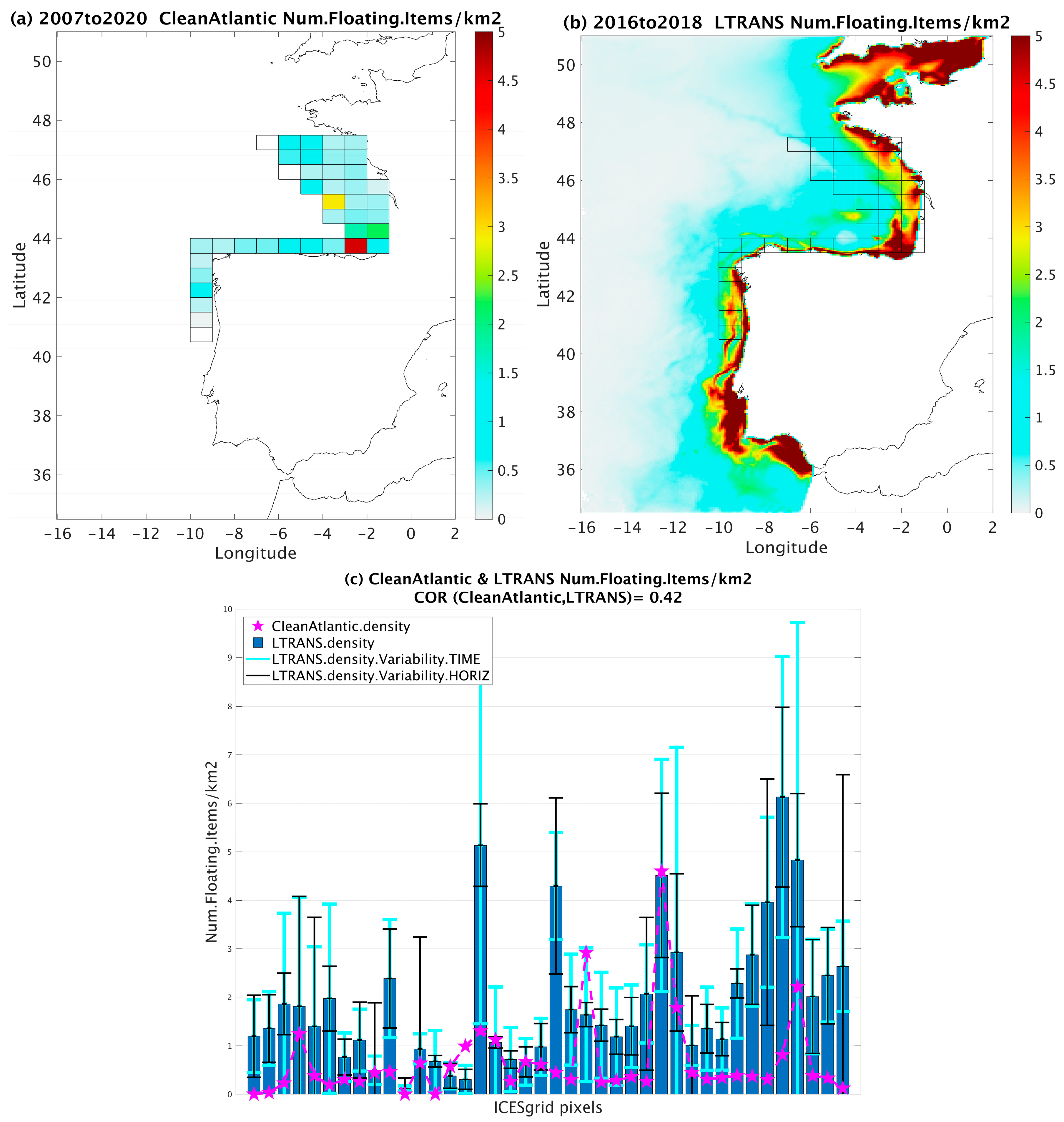
Figure 16a,b show that the CleanAtlantic densities collected in 2007–2020 and the LTRANS densities averaged for 2016–2018 agree in the open ocean grid cells and in detecting the accumulation maximum in the inner Bay of Biscay.

The LTRANS densities indicate several coastal accumulations of marine litter that are not observed by the CleanAtlantic densities. Despite these differences, if the LTRANS results are grouped geographically by the ICES grid cells, the correlation between both is 0.42 (p-value = 0.006).

Figure 16c shows the values of the CleanAtlantic and LTRANS densities by each ICES pixel, together with the variability (or spread in values) of the LTRANS densities in time (light-blue lines) and spatially (black lines) computed for each ICES pixel with the STDs. Again, despite the differences in spatial and time range/resolution between the CleanAtlantic and LTRANS datasets, more than half of the CleanAtlantic values are within the spread of the horizontal and/or time variabilities of LTRANS values.

4. Conclusions

In this study, we address the challenges involved in modelling the spatial distribution and abundances of macroplastic pollution in five EU marine regions with the LTRANS model, and the factors that may condition the estimation of the model accuracy when model results are compared/validated with marine litter observations.

There is an overall good agreement between the LTRANS simulations and the available macroplastic observations in distribution and abundances. This may indicate that the assumptions on the land sources and the estimations of the maritime sources for the EU basins, both forcing the LTRANS runs as inputs, are adequate to obtain realistic results. In the same way, the GETM marine currents and the Stokes Drift from Copernicus are adequate to simulate reasonably the dispersion and accumulation pathways of floating macrolitter.

The comparison of the LTRANS results with available observations reveals that the model’s predictions for both BEACHED and FLOATING macroplastics are generally accurate, although the agreement is more limited in offshore areas. Specifically, the correlations between BEACHED LTRANS predictions and the EMODnet-distributed observations from Member States range from 0.73 to 0.88 in the European basins. In contrast, the correlations for FLOATING macroplastics range from 0.4 to 0.72. This disparity may reflect the fact that the mainland-based sources of macroplastics, largely depending on river observations, are based on more robust and reliable estimates.

In contrast, offshore areas may also be influenced by a range of sources not included here in the LTRANS input data. Whereas the model accounts for the fishing sector, it does not include other potential contributors to floating macroplastics, such as commercial shipping, recreational boating, and direct littering or mismanaged waste in regions not connected to rivers, but that may be relevant in specific open-sea areas. These overlooked sources may be particularly relevant in areas like the Sardinia Channel, where riverine input is minimal but maritime and coastal activity is high, especially during the summer tourist season, which can significantly increase litter loads. As a result, discrepancies between model predictions and field observations may occur in locations such as the transect between Sicily and Sardinia (the Cagliari–Palermo route), where monitoring took place exclusively in summer, a period when litter levels can rise by up to 40%. This seasonal bias likely contributes to the higher observed densities, reflecting peak input periods and underscoring the importance of incorporating temporal and source variability in future model refinements. Additionally, the validation densities were calculated using presence-only data, without accounting for total survey effort or including transects with zero litter observations. This may have led to an overestimation of average densities in some areas, such as the Sardinia Channel, where localized semi-stable gyres promote litter accumulation.

Our analyses of the EMODnet beach-litter data have clearly shown the need to consider the survey periodicity to interpret those data. They do not represent a bulk quantity but rather a flow of material accumulated in the beach during a certain period. The sampling frequency is a key variable to consider if comparisons among monitoring places (or between monitoring and modelling data) are to be performed in a consistent way.

The predicted LTRANS macroplastic densities are of a similar magnitude to available observations, although they tend to be slightly lower. The main factors that can condition the discrepancies between LTRANS predictions and macroplastic observations are the following:

• The comparison of BEACHED LTRANS predictions with EMODnet surveys indicates that the discrepancies between them are mainly located close to ports, river mouths, and coastal lagoons. The LTRANS input sources included may not be releasing enough particles in the basins.
• It could also indicate the lack of some point sources of macroplastic pollution in the model inputs.
• As well, the lower BEACHED LTRANS abundances with respect to the EMODnet observations may also be due to the potential inclusion of land-originated macroplastics that arrived directly from land at the beaches and accounted within the EMODnet surveys.
• The uneven sampling periodicity in many of the beach surveys available may also condition the comparison with the BEACHED LTRANS results.
• Comparing the FLOATING LTRANS results with the available observations indicates that the divergences between them may arise from the intrinsic characteristics of the floating macroplastic data collection at sea used for comparison, which depends on the ship’s availability: observations are available only at specific/scattered locations at sea and with time coordinates unevenly distributed in the time range of the study. On the other hand, in the future, the availability of extensive open-sea observations of floating macroplastics used to improve model inputs will help to increase the accuracy of the FLOATING LTRANS results. These observations would be collected within the frame of projects, such as MEDSEALITTER, that follow a precise protocol for data collection by ships, set up unique strip-width, and allow replicability by a predetermined route-based approach.
• The LTRANS assumption of a homogenous daily release of macroplastics within the month for each source may also condition the accuracy of the LTRANS predictions. Unfortunately, daily realistic input datasets per source location are not available at present.
• Not including fragmentation and sizes of the macroplastics in LTRANS may also contribute to the discrepancies of the model results with observations.

In conclusion, while some discrepancies between model predictions and observed litter densities remain, particularly in offshore areas during peak tourist seasons, the LTRANS model has demonstrated strong potential in representing macroplastic distribution, even in highly dynamic open-sea environments. Our analysis suggests that increasing horizontal model resolution and improving beaching process representation could enhance accuracy. Moreover, incorporating more observational data on sea-based litter sources, especially in high-sea areas, would likely strengthen model performance.

Finally, our study provides a basis for future forecast runs to evaluate the impact of policy/management options on marine macroplastic pollution, since it addresses the challenges involved in modelling the spatial distribution and abundances of macroplastics and the factors that may condition the estimation of the model accuracy when model results are compared/validated with marine litter observations available. In the future, LTRANS model results could inform monitoring efforts under the MSFD by, for example, evaluating the representativeness of selected beaches for monitoring purposes and identifying potential hotspots of pollution that may be overlooked in existing programs. Furthermore, model simulations can be used to estimate the required reduction in litter input necessary to achieve the agreed-upon threshold value of 20 items/100 m on EU coastlines, thereby supporting the development of effective regional action plans and MSFD compliance monitoring.

References

1. Gonzalez-Fernandez, D.; Cozar, A.; Hanke, G.; Viejo, J.; Morales-Caselles, C.; Bakiu, R.; Barcelo, D.; Bessa, F.; Bruge, A.; Cabrera, M.; et al. Floating macrolitter leaked from Europe into the Ocean. Nat. Sustain. 2021, 4, 474–483. [Google Scholar] [CrossRef] [Scilit]
2. Van Sebille, E.; Aliani, S.; Lavender Law, K.; Maximenko, N.; Alsina, J.M.; Bagaev, A.; Bergmann, M.; Chapron, B.; Chubarenko, I.; Cózar, A.; et al. The physical oceanography of the transport of floating marine debris. Environ. Res. Lett. 2020, 15, 023003. [Google Scholar] [CrossRef] [Scilit]
3. Miladinova, S.; Macias, D.; Stips, A.; Garcia-Gorriz, E. Identifying distribution and accumulation patterns of floating marine debris in the Black Sea. Mar. Pollut. Bull. 2020, 153, 110964. [Google Scholar] [CrossRef] [Scilit] [PubMed]
4. Castro-Rosero, L.M.; Hernandez, I.; Alsina, J.M.; Espino, M. Transport and accumulation of floating marine litter in the Black Sea: Insights from numerical modeling. Front. Mar. Sci. 2023, 10, 1213333. [Google Scholar] [CrossRef] [Scilit]
5. Soto-Navarro, J.; Jorda, G.; Deudero, S.; Alomar, C.; Amores, A.; Compa, M. 3D hotspots of marine litter in the Mediterranean: A modeling study. Mar. Pollut. Bull. 2020, 155, 111159. [Google Scholar] [CrossRef] [Scilit]
6. Tsiaras, K.; Hatzonikolakis, Y.; Kalaroni, S.; Pollani, A.; Triantafyllou, G. Modeling the Pathways and Accumulation Patterns of Micro- and Macro-Plastics in the Mediterranean. Front. Mar. Sci. 2021, 8, 743117. [Google Scholar] [CrossRef] [Scilit]
7. Macias, D.; Stips, A.; Hanke, G. Model based estimate of transboundary litter pollution on Mediterranean coasts. Mar. Pollut. Bull. 2022, 175, 113121. [Google Scholar] [CrossRef] [Scilit]
8. Parn, O.; Macias Moy, D.; Stips, A. Determining the distribution and accumulation patterns of floating litter in the Baltic Sea using modelling tools. Mar. Pollut. Bull. 2023, 190, 114864. [Google Scholar] [CrossRef] [Scilit]
9. Christensen, A.; Murawski, J.; She, J.; St. John, M. Simulating transport and distribution of marine macro-plastic in the Baltic Sea. PLoS ONE 2023, 18, e0280644. [Google Scholar] [CrossRef] [Scilit]
10. Madduri, P.; Oleynik, A.; Clark, J.R.; Avlesen, H.; Alendal, G. Modelling transboundary plastic pathways to Norwegian coastal and inland waters. Sci. Total Environ. 2025, 1003, 180582. [Google Scholar] [CrossRef] [Scilit]
11. Macias, D.; Stips, A.; Grizzetti, B.; Aloe, A.; Bisselink, B.; de Meij, A.; De Roo, A.; Duteil, O.; Ferreira-Cordeiro, N.; Garcia-Gorriz, E.; et al. Water/Marine Zero Pollution Outlook: A Forward-Looking, Model-Based Analysis of Water Pollution in the EU; Publications Office of the European Union: Luxembourg, 2022. Available online: https://publications.jrc.ec.europa.eu/repository/handle/JRC131197 (accessed on 26 September 2025).
12. Macias, D.; Cozar, A.; Garcia-Gorriz, E.; González-Fernández, D.; Stips, A. Surface water circulation develops seasonally changing patterns of floating litter accumulation in the Mediterranean Sea: A modelling approach. Mar. Pollut. Bullelltin 2019, 149, 110619. [Google Scholar] [CrossRef] [Scilit]
13. Schlag, Z.R.; North, E.W. Lagrangian TRANSport Model (LTRANS v.2) User’s Guide; University of Maryland Center for Environmental Science, Horn Point Laboratory: Cambridge, MD, USA, 2012; p. 183. Available online: https://northweb.hpl.umces.edu/LTRANS/LTRANS-v2/LTRANSv2_UsersGuide_6Jan12.pdf (accessed on 26 September 2025).
14. Laurent, C.; Querin, S.; Solidoro, C.; Melaku Canu, D. Modelling marine particle dynamics with LTRANS-Zlev: Implementation and validation. Environ. Model. Softw. 2020, 125, 104621. [Google Scholar] [CrossRef] [Scilit]
15. Dobler, D.; Huck, T.; Maes, C.; Grima, N.; Blanke, B.; Martinez, E.; Ardhuin, F. Large impact of Stokes drift on the fate of surface floating debris in the South Indian Basin. Mar. Pollut. Bull. 2019, 148, 202–209. [Google Scholar] [CrossRef] [Scilit] [PubMed]
16. Bosi, S.; Brostrom, G.; Roquet, F. The Role of Stokes Drift in the Dispersal of North Atlantic Surface Marine Debris. Front. Mar. Sci. 2021, 8, 697430. [Google Scholar] [CrossRef] [Scilit]
17. Stips, A.; Bolding, K.; Pohlman, T.; Burchard, H. Simulating the temporal and spatial dynamics of the North Sea using the new model GETM (General Estuarine Transport Model). Ocean. Dyn. 2004, 54, 266–283. [Google Scholar] [CrossRef] [Scilit]
18. Schmidt, C.; Krauth, T.; Wagner, S. Export of plastic debris by rivers into the sea. Environ. Sci. Technol. 2017, 51, 12246–12253. [Google Scholar] [CrossRef] [Scilit]
19. Gonzalez-Fernandez, D.; Hanke, G. Toward a Harmonized Approach for Monitoring of Riverine Floating Macro Litter Inputs to the Marine Environment. Front. Mar. Sci. 2017, 4, 86. [Google Scholar] [CrossRef] [Scilit]
20. Jambeck, J.R.; Geyer, R.; Wilcox, C.; Siegler, T.R.; Perryman, M.; Andrady, A.; Narayan, R.; Lavender Law, K. Plastic waste inputs from land into the ocean. Science 2015, 347, 768–771. [Google Scholar] [CrossRef] [Scilit]
21. Muñoz-Sabater, J. ERA5-Land Monthly Averaged Data from 1981 to Present. Copernicus Climate Change Service (C3S). Climate Data Store (CDS). 2019. Available online: https://cds.climate.copernicus.eu/datasets/reanalysis-era5-land-monthly-means?tab=overview (accessed on 1 March 2023). [CrossRef]
22. GESAMP. Sea-Based Sources of Marine Litter; Gilardi, K., Ed.; IMO/FAO/UNESCO-IOC/UNIDO/ WMO/IAEA/UN/UNEP/UNDP/ISA Joint Group of Experts on the Scientific Aspects of Marine Environmental Protection: London, UK, 2021; Volume 108, 109p.
23. Arcadia Marine Initiative. Annual Report. 2013. Available online: https://www.fauna-flora.org/ (accessed on 1 June 2023).
24. Sherrington, C.; Darrah, C.; Hann, S.; Cole, G.; Corbin, M. Study to Support the Development of Measures to Combat a Range of Marine Litter Sources; Report for European Commission DG Environment by Eunomia Research & Consulting Ltd.; European Commission DG Environment by Eunomia Research & Consulting Ltd.: Bristol, UK, 2021; Available online: https://www.kosmopedia.org/wp-content/uploads/2020/09/MSFD-Measures-to-Combat-Marine-Litter.pdf (accessed on 1 June 2023).
25. STECF-Scientific, Technical and Economic Committee for Fisheries. The 2014 Annual Economic Report on the EU Fishing Fleet (STECF-14-16); Publications Office of the European Union: Luxembourg, 2014.
26. Vinci, M.; Giorgetti, A.; Lipizer, M. The Role of EMODnet Chemistry in the European Challenge for Good Environmental Status. Nat. Hazards Earth Syst. Sci. 2017, 17, 197–204. [Google Scholar] [CrossRef] [Scilit]
27. Molina Jack, M.E.; Altenburger, A.; Caer, G.; Cociancich, A.; Fortibuoni, T.; Galgani, F.; Giorgetti, A.; Partescano, E.; Thomas, A.; Vinci, M.A. Mediterranean Focus Overview of EU Marine Litter Data Management Performed in the Framework of the European Marine Observation and Data Network Chemistry. Sustainability 2023, 15, 16490. [Google Scholar] [CrossRef] [Scilit]
28. Galgani, F.; Hanke, G.; Werner, S.; Oosterbaan, L.; Nilsson, P.; Fleet, D.; Kinsey, S.; Thompson, R.C.; van Franeker, J.; Vlachogianni, T.; et al. Guidance on Monitoring of Marine Litter in European Seas; JRC EUR 26113 EN; European Commission, Joint Research Centre, Publications Office of the European Union: Luxembourg, 2013. [CrossRef]
29. Galgani, F.; Giorgetti, A.; Le Moigne, M.; Brosich, A.; Vinci, M.; Lipizer, M.; Molina Jack, M.E.; Holdsworth, N.; Schlitzer, R.; Hanke, G.; et al. Guidelines and Forms for Gathering Marine Litter Data: Beach and Seafloor Trawlings; Version 7.1; EMODnet: Oostende, Belgium, 2022; 72p, Available online: https://repository.oceanbestpractices.org/items/cb5027b3-7ea4-4125-8e8f-aade2c74a78c (accessed on 26 September 2025).
30. Galgani, F.; Ruiz-Orejón, L.F.; Ronchi, F.; Tallec, K.; Fischer, E.K.; Matiddi, M.; Anastasopoulou, A.; Andresmaa, E.; Angiolillo, M.; Bakker Paiva, M.; et al. Guidance on the Monitoring of Marine Litter in European Seas: An Update to Improve the Harmonised Monitoring of Marine Litter Under the Marine Strategy Framework Directive; MSFD Technical Group on Marine Litter; EUR 31539 EN; Publications Office of the European Union: Luxembourg, 2023; ISBN 978-92-68-04093-5. [CrossRef]
31. MEDSEALITTER Partners. MEDSEALITTER: Common Monitoring Protocol for Marine Litter; Publications Office of the European Union: Luxembourg, 2019. Available online: https://medasset.org/wp-content/uploads/2019/05/MEDSEALITTER_Shared-monitoring-protocol_FINAL.pdf (accessed on 26 September 2025).
32. Thiel, M.; Hinojosa, I.; Vasquez, N.; Macaya, E. Floating marine debris in coastal waters of the SE-Pacific (Chile). Mar. Pollut. Bull. 2003, 46, 224–231. [Google Scholar] [CrossRef] [Scilit]
33. Joint Black Sea Surveys 2017, 2018. National Pilot Monitoring Studies and Joint Open Sea Surveys in Georgia, Russian Federation and Ukraine, 2017. Available online: http://emblasproject.org/publications-reports (accessed on 1 December 2024).
34. Gonzalez-Fernandez, D.; Hanke, G.; Pogojeva, M.; Machitadze, N.; Kotelnikova, Y.; Tretiak, I.; Savenko, O.; Bilashvili, K.; Gelashvili, N.; Fedorov, A.; et al. Floating marine macro litter in the Black Sea: Toward baselines for large scale assessment. Environ. Pollut. 2022, 309, 119816. [Google Scholar] [CrossRef] [Scilit]
35. CleanAtlantic Partners. CleanAtlantic. Tackling Marine Litter in the Atlantic Area. 2021. Available online: https://www.cleanatlantic.eu/wp-content/uploads/2021/12/WP4-1_FloatingLitter-AA-VF.pdf (accessed on 1 December 2024).
36. Hengstmann, E.; Gräwe, D.; Tamminga, M.; Kerstin Fischer, E. Marine litter abundance and distribution on beaches on the Isle of Rugen considering the influence of exposition, morphology and recreational activities. Mar. Pollut. Bull. 2017, 115, 297–306. [Google Scholar] [CrossRef] [Scilit]
Figure 1. The five European marine basins as defined in this work. NWES stands for the Atlantic Northwest European Shelf domain, and SWES for the Atlantic Southwest European Shelf domain.
Oceans 07 00026 g001
Figure 2. Macroplastic input estimates (millions of macroplastics/year) for all EU marine regions in the present day (2018 as reference year) computed by the model in [1].
Oceans 07 00026 g002
Figure 3. Fishing vessel density for year 2018 as contained in EMODnet VMS dataset.
Oceans 07 00026 g003
Figure 4. LTRANS beached times plotted with the corresponding EMODnet survey periodicities for each country in (a) the Baltic Sea, (b) the Black Sea, (c) the Mediterranean Sea, (d) the NWES, and (e) the SWES basin (b). The size of the colored circles indicates the number of EMODnet surveys per country, with the STD of the EMODnet periodicities in horizontal bars to inform about the range of survey periodicities used by the EMODnet observers.
Oceans 07 00026 g004
Figure 5. (a) EMODnet macroplastics/100 m in the Baltic Sea for the surveys from 2016 to 2018 with survey periodicity less or equal to 6 months. (b) LTRANS macroplastics/100 m for the same dates and locations of the EMODnet surveys. In (a) and (b), both color and diameter of the circles visualize the number of macroplastics/100 m.
Oceans 07 00026 g005
Figure 6. Same as in Figure 5, for the Black Sea.
Oceans 07 00026 g006
Figure 7. Same as in Figure 5, for the Mediterranean Sea.
Oceans 07 00026 g007
Figure 8. Same as Figure 5, for the NWES basin.
Oceans 07 00026 g008
Figure 9. Same as in Figure 5, for the SWES basin.
Oceans 07 00026 g009
Figure 10. The correlations of EMODnet and LTRANS plotted with the corresponding maximum value of the horizontal resolutions (km) for each basin. The y-axis direction is reverse, with the coarser resolutions at the bottom and the finer resolutions at the top. The dashed line shows the linear fit if the German and Greek EMODnet sites are excluded of the correlation calculation by basin.
Oceans 07 00026 g010
Figure 11. Mean correlations between MEDSEALITTER and the LTRANS floating macroplastics densities, assuming time tolerances of ±0, ±1, ±2, and ±3 days and horizontal tolerances of ±0, ±1, ±2, and ±3 pixels in the LTRANS day maps, with respect to the percentage of observations included in the calculation. The color and size of the circles indicate the mean density of floating macroplastics for each case. The red circle on the top right corner is the corresponding MEDSEALITTER density according to the observations included in the 2d2p case. The histograms show the number of best-fit LTRANS densities that are within ±0, ±1, ±2, and ±3 pixels for cases 2d2p and 3d3p.
Oceans 07 00026 g011
Figure 12. Geographical distribution of the MEDSEALITTER densities time averaged for the 3 years for the 2d2p comparison case. The color and size of the circles indicate the densities computed with observed strip-widths.
Oceans 07 00026 g012
Figure 13. Geographical distribution of the LTRANS densities time averaged for the 3 years for the 2d2p comparison case.
Oceans 07 00026 g013
Figure 14. Geographical distribution of the 3-year-averaged MEDSEALITTER-LTRANS correlations for the comparison case 2p2d (colored circles). They are overlapping the map of the variability (or STD) of the 3-year LTRANS densities (plotted with the grey colorbar).
Oceans 07 00026 g014
Figure 15. Number of macroplastics per km2 in November 2017: map of LTRANS floating macroplastics plotted together with the EMBLAS observations in the boxed numbers. The colors in the map and the colors of the boxed numbers share the same color-scale on the right-hand side to facilitate the comparison.
Oceans 07 00026 g015
Figure 16. (a) Map of CleanAtlantic floating-litter densities in the ICES grid, including observations collected in different oceanographic surveys at specific times between 2007 and 2020. (b) Map of the LTRANS densities averaged from 2016 to 2018. The locations of the ICES pixels in a) are indicated in b) with the corresponding black rectangles. (c) Comparison between the CleanAtlantic and LTRANS densities by each ICES-pixel. The magenta stars are the CleanAtlantic densities, and the dark-blue bars are the corresponding LTRANS densities. The LTRANS density variability in time (light-blue lines) and spatially (black lines) is computed with the STDs.
Oceans 07 00026 g016